How to copy cells with formulas in excel

Move or copy cells and cell contents

Use Cut, Copy, and Paste to move or copy cell contents. Or copy specific contents or attributes from the cells. For example, copy the resulting value of a formula without copying the formula, or copy only the formula.

When you move or copy a cell, Excel moves or copies the cell, including formulas and their resulting values, cell formats, and comments.

You can move cells in Excel by drag and dropping or using the Cut and Paste commands.

Move cells by drag and dropping

Select the cells or range of cells that you want to move or copy.
Point to the border of the selection.
When the pointer becomes a move pointer , drag the cell or range of cells to another location.

Move cells by using Cut and Paste

Select a cell or a cell range.
Select Home > Cut or press Ctrl + X.
Select a cell where you want to move the data.
Select Home > Paste or press Ctrl + V.

Copy cells by using Copy and Paste

Select the cell or range of cells.
Select Copy or press Ctrl + C.
Select Paste or press Ctrl + V.

Need more help?

You can always ask an expert in the Excel Tech Community or get support in the Answers community.

Copy and Paste Formulas in Excel without Changing Cell References

When using relative/mixed references in your formulas, you may – sometimes – want to copy and paste formulas in Excel without changing the cell references.

Simply put, you want to copy the exact formula from one set of cells to another.

In this tutorial, I will show you how you can do this using various ways:

Manually Copy Pasting formulas.
Using ‘Find and Replace’ technique.
Using the Notepad.

Manually Copy Paste the Exact Formula

If you only have a handful of formulas that you want to copy and paste without changing the cell references, doing it manually would be more efficient.

To copy paste formulas manually:

Select the cell from which you want to copy the formula.
Go to the formula bar and copy the formula (or press F2 to get into the edit mode and then copy the formula).
Select the destination cell and paste the formula.

Note that this method works only when you have a few cells from which you want to copy formulas.

If you have a lot, use the find and replace technique shown below.

Using Find and Replace

Here are the steps to copy formulas without changing the cell references:

This will convert the text back into the formula and you will get the result.

Note: If you use the # character as a part of your formula, you can use any other character in Replace with (such as ‘ZZZ’ or ‘ABC’).

Using Notepad to Copy Paste Formulas

If you have a range of cells where you have the formulas that you want to copy, you can use a Notepad to quickly copy and paste the formulas.

Here are the steps to copy formulas without changing the cell references:

Go to Formulas –> Show Formulas. This will show all the formulas in the worksheet.
Copy the cells that have the formulas that you want to copy.
Open a notepad and paste the cell contents in the notepad.
Copy the content on the notepad and paste in the cells where you want the exact formulas copied.
Again go to Formulas –> Show formulas.

Note: Instead of Formulas –> Show formulas, you can also use the keyboard shortcut Control + ` (this is the same key that has the tilde sign).

You May Also Like the Following Tutorials:

How to Convert Formulas to Values in Excel.
Show Formulas in Excel Instead of the Values.
How to Lock Formulas in Excel.
Understanding Absolute, Relative, and Mixed Cell References in Excel.
How to reference another sheet in Excel.
How to Remove Cell Formatting in Excel
How to Copy Excel Table to Word
How to Copy and Paste Column in Excel?
How to Multiply a Column by a Number in Excel

Get 51 Excel Tips Ebook to skyrocket your productivity and get work done faster

31 thoughts on “How to Copy and Paste Formulas in Excel without Changing Cell References”

Thank you for your help.
“Using Find and Replace” is very good option. it really works.
Thank you very much
BROOOOOO! This was so smart and easy. Thanks my friend!
Excellent. That has made my work today so much easier!!
Thanks you so much! This Helped me a lot!!
Great! Thanks for the teaching! Loving the Notepad method
Amazing….such a nice n easy way to do it with replace..thanks a lot
Thanks alot. really helpful
Nice. Very well explained, thank you.
OH. MY. GOSH. I’m 10 hours of copying and pasting formulas but this has saved me at least a few more and countless future hours! Replacing = with #, pasting, then replacing # with =. It’s so simple… why didn’t I think of it. 🙂 Thank you!
Thanks a lot Simple & Eazy
# is best and easiest solution, thanks a lot!!! very clever!
thanks a lot
This saved me tonnes of work. Thanks so much!
For a copying and pasting a large array of formulas comprising both relative and absolute references to different cells, sheets and workbooks, the ‘find and replace’ has proven to be convoluted, time consuming and problematic. One has to ‘cherry pick’ through the array to ensure which of one’s relative cell references are not to be changed.
I migrated to excel from lotus-123; as a comparison using ‘123’ back then, one would simply ‘highlight rows (or columns)’, ‘copy’, ‘insert’ equal rows (or columns), then ‘paste’ – quick and most importantly no cherry picking errors.
Excel’s ‘insert copied cells’ command hides the ‘insert row or column’ command, therefore one cannot emulate the ‘123’ way. Even if one tries the ‘insert sheet rows (or columns)’ command then attempt to paste directly from ‘clipboard’, only text and not formulas are pasted.
amazing!
thanks
saved me 20 min. of work…
THIS IS AWESOME! – THE # = TRICK. GENIUS!
THANK U VERY MUCH!
- Agree! This is so simple, but very helpful. Thanks!
I have a cell reference issue I hope someone can help me with. I have a cell outside of a range that I always want to refer to a specific cell inside of the range, even when cells are inserted or deleted from the range. For example, cell A10 refers to C10 in the range B1:D200. If someone inserts cells B7:D13, I still want A10 to refer to C10, not C17. I think I need a helper column that has the text “C10” in cell E10. What is the Function that gets A10 to use the static text in E10 to refer to cell C10?
- You can use the INDIRECT function. This should work =INDIRECT(“C10”). If you have text C10 in cell E10, just use =INDIRECT(E10)
  - Thanks. That is the Function I was looking for, but could not remember.
  - Even though INDIRECT is less complicated, can you tell me why CELL(“contents”,ADDRESS(10,3)) didn’t work?
    - Jim,
      although these are functions I’ve never had cause to use, I think this might be because the $C$10 from the ADDRESS function is seen as text, not a cell reference
      CELL(“contents”,”$C$10″) certainly does not work
      regards,
      t’other jim
  - although INDIRECT is the way to go with this, you could also use OFFSET:
    =OFFSET(A10,,2) should work
    both are volatile formulae (will recalculate on every worksheet change), which you might be able to avoid by using =INDEX(C:C,10) which would only fail your requirements if a whole column were inserted or deleted somewhere between A:A and C:C
    - taking this a step further, =INDEX(1:1048576,10,3) will always refer to C10 – but it’s very clumsy-looking
- I’ve made a step in the right direction. ADDRESS(10,3) results in $C$10 and it does not change when cell C10 is moved. CELL(“contents”,$C$10) gives me the proper result. However, CELL(“contents”,ADDRESS(10,3)) is not even accepted. What is wrong with the nested formula?
  - you should use “=CELL(“contents”, INDIRECT(ADDRESS(10,3,1,1,”Sheet1″),1))” as there are certain arguments to ADDRESS function which ADDRESS(10,3) is not capturing and those arguments are not optional.
I think Bansal’s point was that sometimes you can have a range of dynamic formulae that you want to replicate elsewhere
I’ve had this situation occur before but I never thought of using the Notepad method – thanks for that, another weapon in my arsenal
Absolute cell reference is the best. i.e. =A$1$ + B$1$ this cell is locked in that way.
I use absolute/Dynamic references for doing this
- I love method 3. Thanks you.

Comments are closed.

Источник

Download Article

Using Find and Replace

Filling a Column or Row

Pasting a Formula into Multiple Cells

Using Relative and Absolute Cell References

Video

Tips

Warnings

Excel makes it easy to copy your formula across an entire row or column, but you don’t always get the results you want. If you end up with unexpected results, or those awful #REF and /DIV0 errors, it can be extremely frustrating. But don’t worry—you won’t need to edit your 5,000 line spreadsheet cell-by-cell. This wikiHow teaches you easy ways to copy formulas to other cells.

Open your workbook in Excel. Sometimes, you have a large spreadsheet full of formulas, and you want to copy them exactly. Changing everything to absolute cell references would be tedious, especially if you just want to change them back again afterward. Use this method to quickly move formulas with relative cell references elsewhere without changing the references.^[1] In our example spreadsheet, we want to copy the formulas from column C to column D without changing anything.

Example Spreadsheet

	Column A	Column B	Column C
row 1	944	Frogs	=A1/2
row 2	636	Toads	=A2/2
row 3	712	Newts	=A3/2
row 4	690	Snakes	=A4/2

If you’re just trying to copy the formula in a single cell, skip to the last step («Try alternate methods») in this section.

2

Press Ctrl+H to open the Find window. The shortcut is the same on Windows and macOS.

Advertisement

Find and replace «=» with another character. Type «=» into the «Find what» field, and then type a different character into the «Replace with» box. Click Replace All to turn all formulas (which always begin with an equal’s sign) into text strings beginning with some other character. Always use a character that you have not used in your spreadsheet. For example, replace it with # or &, or a longer string of characters, such as ##&.

Example Spreadsheet

	Column A	Column B	Column C
row 1	944	Frogs	##&A1/2
row 2	636	Toads	##&A2/2
row 3	712	Newts	##&A3/2
row 4	690	Snakes	##&A4/2

Do not use the characters * or ?, since these will make later steps more difficult.

Copy and paste the cells. Highlight the cells you want to copy, and then press Ctrl + C (PC) or Cmd + C (Mac) to copy them. Then, select the cells you want to paste into, and press Ctrl + V (PC) or Cmd + V (Mac) to paste. Since they are no longer interpreted as formulas, they will be copied exactly.

Example Spreadsheet

	Column A	Column B	Column C	Column D
row 1	944	Frogs	##&A1/2	##&A1/2
row 2	636	Toads	##&A2/2	##&A2/2
row 3	712	Newts	##&A3/2	##&A3/2
row 4	690	Snakes	##&A4/2	##&A4/2

Use Find & Replace again to reverse the change. Now that you have the formulas where you want them, use «Replace All» again to reverse your change. In our example, we’ll look for the character string «##&» and replace it with «=» again, so those cells become formulas once again. You can now continue editing your spreadsheet as usual:

Example Spreadsheet

	Column A	Column B	Column C	Column D
row 1	944	Frogs	=A1/2	=A1/2
row 2	636	Toads	=A2/2	=A2/2
row 3	712	Newts	=A3/2	=A3/2
row 4	690	Snakes	=A4/2	=A4/2

6
Try alternate methods. If the method described above doesn’t work for some reason, or if you are worried about accidentally changing other cell contents with the «Replace all» option, there are a couple other things you can try:
- To copy a single cell’s formula without changing references, select the cell, then copy the formula shown in the formula bar near the top of the window (not in the cell itself). Press Esc to close the formula bar, then paste the formula wherever you need it.
- Press Ctrl and ` (usually on the same key as ~) to put the spreadsheet in formula view mode. Copy the formulas and paste them into a text editor such as Notepad or TextEdit. Copy them again, then paste them back into the spreadsheet at the desired location. Then, press Ctrl and ` again to switch back to regular viewing mode.

Type a formula into a blank cell. Excel makes it easy to propagate a formula down a column or across a row by «filling» the cells. As with any formula, start with an = sign, then use whichever functions or arithmetic you’d like. We’ll use a simple example spreadsheet, and add column A and column B together. Press Enter or Return to calculate the formula.

Example Spreadsheet

	Column A	Column B	Column C
row 1	10	9	19
row 2	20	8
row 3	30	7
row 4	40	6

2

Click the lower right corner of the cell with the formula you want to copy. The cursor will become a bold + sign.

Click and drag the cursor across the column or row you’re copying to. The formula you entered will automatically be entered into the cells you’ve highlighted. Relative cell references will automatically update to refer to the cell in the same relative position rather than stay exactly the same. Here’s our example spreadsheet, showing the formulas used and the results displayed:

Example Spreadsheet

	Column A	Column B	Column C
row 1	10	9	=A1+B1
row 2	20	8	=A2+B2
row 3	30	7	=A3+B3
row 4	40	6	=A4+B4

Example Spreadsheet

	Column A	Column B	Column C
row 1	10	9	19
row 2	20	8	28
row 3	30	7	37
row 4	40	6	46

You can also double-click the plus sign to fill the entire column instead of dragging. Excel will stop filling out the column if it sees an empty cell. If the reference data contains a gap, you will have to repeat this step to fill out the column below the gap.
Another way to fill the entire column with the same formula is to select the cells directly below the one containing the formula and then press Ctrl + D.^[2]

Type the formula into one cell. As with any formula, start with an = sign, then use whichever functions or arithmetic you’d like. We’ll use a simple example spreadsheet, and add column A and column B together. When you press Enter or Return, the formula will calculate.

Example Spreadsheet

	Column A	Column B	Column C
row 1	10	9	19
row 2	20	8
row 3	30	7
row 4	40	6

2

Select the cell and press Ctrl+C (PC) or ⌘ Command+C (Mac). This copies the formula to your clipboard.
3

Select the cells you want to copy the formula to. Click on one and drag up or down using your mouse or the arrow keys. Unlike with the column or row fill method, the cells you are copying the formula to do not need to be adjacent to the cell you are copying from. You can hold down the Control key while selecting to copy non-adjacent cells and ranges.
4

Press Ctrl+V (PC) or ⌘ Command+V (Mac) to paste. The formulas now appear in the selected cells.

Use a relative cell reference in a formula. In an Excel formula, a «cell reference» is the address a cell. You can type these in manually, or click on the cell you wish to use while you are entering a formula. For example, the following spreadsheet has a formula that references cell A2:

Relative References

	Column A	Column B	Column C
row 2	50	7	=A2*2
row 3	100
row 4	200
row 5	400

2
Understand why they’re called relative references. In an Excel formula, a relative reference uses the relative position of a cell address. In our example, C2 has the formula “=A2”, which is a relative reference to the value two cells to the left. If you copy the formula into C4, then it will still refer to two cells to the left, now showing “=A4”.

Relative References

Column A Column B Column C

row 2
50

7

=A2*2

row 3
100

row 4
200

=A4*2

row 5
400
- This works for cells outside of the same row and column as well. If you copied the same formula from cell C1 into cell D6 (not shown), Excel would change the reference «A2» to a cell one column to the right (C→D) and 5 rows below (2→7), or «B7».
3
Use an absolute reference instead. Let’s say you don’t want Excel to automatically change your formula. Instead of using a relative cell reference, you can make it absolute by adding a $ symbol in front of the column or row that you want to keep the same, no matter where you copy the formula too.^[3] Here are a few example spreadsheets, showing the original formula in larger, bold text, and the result when you copy-paste it to other cells:
- Relative Column, Absolute Row (B$3): The formula has an absolute reference to row 3, so it always refers to row 3:
  
  Column A Column B Column C
  
  row 1
  50
  
  7
  
  =B$3
  
  row 2
  100
  
  =A$3
  
  =B$3
  
  row 3
  200
  
  =A$3
  
  =B$3
  
  row 4
  400
  
  =A$3
  
  =B$3
- Absolute Column, Relative Row ($B1): The formula has an absolute reference to column B, so it always refers to column B.
  
  Column A Column B Column C
  
  row 1
  50
  
  7
  
  =$B1
  
  row 2
  100
  
  =$B2
  
  =$B2
  
  row 3
  200
  
  =$B3
  
  =$B3
  
  row 4
  400
  
  =$B4
  
  =$B4
- Absolute Column & Row ($B$1): The formula has an absolute reference to column B of row 1, so it always refers to column B of row 1.
  
  Column A Column B Column C
  
  row 1
  50
  
  7
  
  =$B$1
  
  row 2
  100
  
  =$B$1
  
  =$B$1
  
  row 3
  200
  
  =$B$1
  
  =$B$1
  
  row 4
  400
  
  =$B$1
  
  =$B$1
4

Use the F4 key to switch between absolute and relative. Highlight a cell reference in a formula by clicking it and press F4 to automatically add or remove $ symbols. Keep pressing F4 until the absolute or relative references you’d like are selected, then press Enter or Return.

	Column A	Column B	Column C
row 1	50	7	=B$3
row 2	100	=A$3	=B$3
row 3	200	=A$3	=B$3
row 4	400	=A$3	=B$3

	Column A	Column B	Column C
row 1	50	7	=$B1
row 2	100	=$B2	=$B2
row 3	200	=$B3	=$B3
row 4	400	=$B4	=$B4

	Column A	Column B	Column C
row 1	50	7	=$B$1
row 2	100	=$B$1	=$B$1
row 3	200	=$B$1	=$B$1
row 4	400	=$B$1	=$B$1

Add New Question

Question

When I try to pull down formula, it stays the same and does not change with row, what can I do?

Go to Formulas, Calculation Options, and change them from Manual to Automatic.
Question

When I click and drag, it copies the format also. I don’t want to copy the format, just the formula?

Krisztian Toth

Community Answer

Right after the drag there should be an icon in the lower right corner of the highlighted area. Hover over that and select from the various fill options, among which you can find an option to fill without format.
Question

How do I copy a date formula I have created (that includes the week day as well as date) so that it runs in sequence?

Krisztian Toth

Community Answer

Double click into the cell, copy your formula, double click into the destination cell, then press Ctrl+V or Command+V.

Ask a Question

200 characters left

Include your email address to get a message when this question is answered.

Submit

If you copy a formula to a new cell and see a green triangle, Excel has detected a possible error. Examine the formula carefully to see if anything went wrong.^[4]
If you accidentally did replace the = character with ? or * in the «copying a formula exactly» method, searching for «?» or «*» will not give you the results you expect. Correct this by searching for «~?» or for «~*» instead.^[5]
Select a cell and press Ctrl‘ (apostrophe) to fill it with the formula directly above it.

Thanks for submitting a tip for review!

Different versions of Excel may not show exactly the same screenshots in the same ways as are displayed here.

References

About This Article

Article SummaryX

To copy a formula into multiple adjoining cells in Microsoft Excel, type the formula into a cell, and then press Enter or Return to calculate it. Hover your mouse cursor over the bottom-right corner of the cell so the cursor turns to a crosshair, then drag the crosshair down to copy the formula to other cells in the column. If you’d rather copy the formula to cells in a row, drag the crosshair left or right.
To copy a formula to cells that aren’t touching the formula cell, click the cell once to select it, and then press Control + C (on a PC) or Command + C (on a Mac) to copy the formula. Now, select the cell or cells you want to copy the formula to, then press Control + V (on a PC) or Command + V (on a Mac) to paste it into the selected cells.

Did this summary help you?

Thanks to all authors for creating a page that has been read 513,635 times.

Is this article up to date?

Источник

Working in spreadsheets all day? Check out these 15 copy & paste tricks to save time when you’re copying and pasting cells in Microsoft Excel.

Excel is one of the most intuitive spreadsheet applications to use. But when it comes to copying and pasting data throughout different parts of the spreadsheet, most users don’t realize how many possibilities there are.

Whether you want to copy and paste individual cells, rows or columns, or entire sheets, the following 15 tricks will help you do it faster and more efficiently.

1. Copy Formula Results

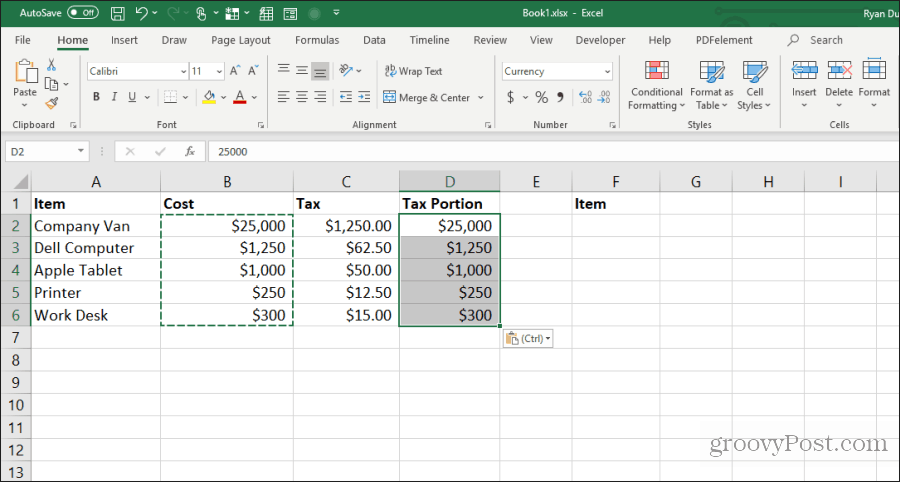
One of the most annoying things about copying and pasting in Excel is when you try to copy and paste the results of Excel formulas. This is because, when you paste formula results, the formula automatically updates relative to the cell you’re pasting it into.

You can prevent this from happening and copy only the actual values using a simple trick.

Select the cells with the values you want to copy. Right-click any of the cells and select Copy from the pop-up menu.

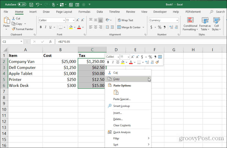
Right-click the first cell in the range where you want to paste the values. Select the Values icon from the pop-up menu.

This will paste only the values (not the formulas) into the destination cells.

This removes all of the relative formula complexity when you normally copy and paste formula cells in Excel.

2. Copy Formulas Without Changing References

If you want to copy and paste formula cells but keep the formulas, you can do this as well. The only problem with strictly pasting formulas is that Excel will automatically update all the referenced cells relative to where you’re pasting them.

You can paste the formula cells but keep the original referenced cells in those formulas by following the trick below.

Highlight all of the cells that contain the formulas you want to copy. Select the Home menu, click on the Find & Select icon in the Editing group, and select Replace.

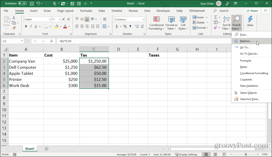
In the Find and Replace window, type = in the Find what field, and # in the Replace with field. Select Replace All. Select Close.

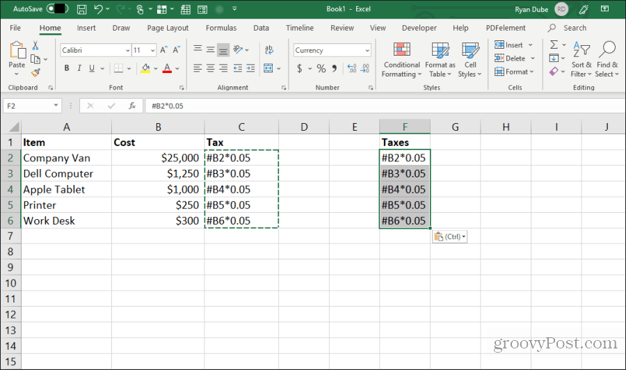
This will convert all formulas to text with the # sign at the front. Copy all of these cells and paste them into the cells where you want to paste them.

Next, highlight all of the cells in both columns. Hold down the Shift key and highlight all cells in one column. Then hold down the Control key and select all of the cells in the pasted column.

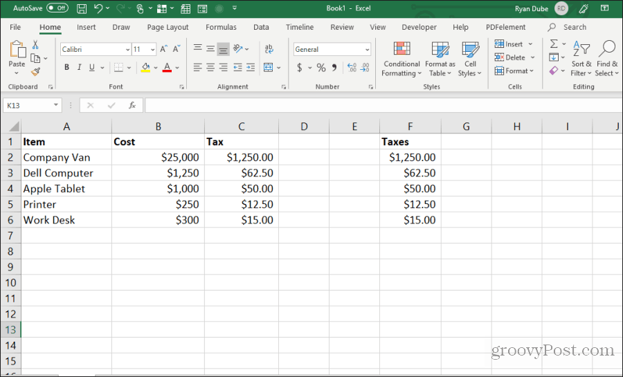
With all cells still highlighted, repeat the search and replace procedure above. This time, type # in the Find what field, and = in the Replace with field. Select Replace All. Select Close.

Once the copy and replace are done, both ranges will contain the same formulas without shifting references.

This procedure may seem like a few extra steps, but it’s the easiest to override the updated references in copied formulas.

3. Avoid Copying Hidden Cells

Another common annoyance when copying and pasting in Excel is when hidden cells get in the way when you copy and paste. If you select and paste those cells, you’ll see the hidden cell appear in the range where you paste them.

If you only want to copy and paste the visible cells, select the cells. Then in the Home menu, select Find & Select, and then select Go To Special from the dropdown menu.

In the Go To Special window, enable Visible cells only. Select OK.

Now press Control+C to copy the cells. Click on the first cell where you want to paste, and press Control+V.

This will paste only the visible cells.

Note: Pasting the cells into a column where an entire second row is hidden will actually hide the second visible cell you’ve pasted.

4. Fill to Bottom with Formula

If you’ve entered a formula into a top cell next to a range of cells already filled out, there’s an easy way to paste the same formula into the rest of the cells.

The typical way people do this is to click and hold the handle on the bottom left of the first cell and drag it to the bottom of the range. This will fill in all cells and update cell references in the formulas accordingly.

But if you have thousands of rows, dragging all the way to the bottom can be difficult.

Instead, select the first cell, then hold down the Shift key and hover the house over the lower-right handle on the first cell until you see two parallel lines appear.

Double click on this double-line handle to fill to the bottom of the column with data to the left.

This technique to fill cells down is fast and easy and saves a lot of time when you’re dealing with extensive spreadsheets.

5. Copy Using Drag and Drop

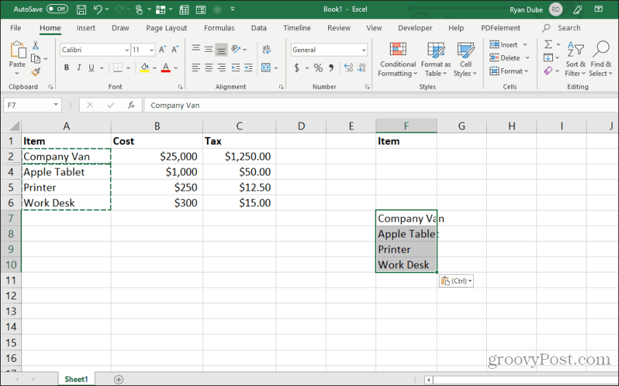
Another neat time-saver is copying a group of cells by dragging and dropping them across the sheet. Many users don’t realize that you can move cells or ranges just by clicking and dragging.

Give this a try by highlighting a group of cells. Then hover the mouse pointer over the edge of the selected cells until it changes to a crosshair.

Left-click and hold the mouse to drag the cells to their new location.

This technique performs the same action as using Control-C and Control-V to cut and paste cells. It’ll save you a few keystrokes.

6. Copy from Cell Above

Another quick trick to save keystrokes is the Control+D command. If you place the cursor under the cell, you want to copy, press Control+D, and the cell above will get copied and pasted into the cell you’ve selected.

Control+Shift+’ performs the same action as well.

7. Copy from Left Cell

If you want to do the same thing but copying from the cell to the left instead, select the cell to the right and press Control+R.

This will copy the cell to the left and paste it in the cell to the right, with just one keystroke!

8. Copy Cell Formatting

Sometimes, you may want to use the same formatting in other cells that you’ve used in an original cell. However, you don’t want to copy the contents.

You can copy just the formatting of a cell by selecting the cell, then type Control+C to copy.

Select the cells you want to format like the original, right-click, and select the formatting icon.

This will paste only the original formatting but not the content.

9. Copy Entire Sheet

If you’ve ever wanted to work with a spreadsheet but didn’t want to mess up the original sheet, copying the sheet is the best approach.

Doing this is easy. Don’t bother to right-click and select Move or Copy. Save a few keystrokes by holding down the Control key, left-click on the sheet tab, and dragging it to the right or the left.

You’ll see a small sheet icon appear with a + symbol. Release the mouse button, and the sheet will copy where you’ve placed the mouse pointer.

10. Repeat Fill

If you have a series of cells that you want to drag down a column and have those cells repeat, doing so is simple.

Just highlight the cells that you want to repeat. Hold down the Control key, left-click the lower right corner of the bottom cell, and drag down the number of cells that you’d like to repeat.

This will fill all of the cells below the copied ones in a repeating pattern.

11. Paste Entire Blank Column or Row

Another trick to save keystrokes is adding blank columns or rows.

The typical method users use to do this is right-clicking the row or column where they want a blank and selecting Insert from the menu.

A faster way is to highlight the cells that make up the row or column of data where you need the blank.

Holding down the Shift key, left-click the bottom right corner of the selection, and drag down (or to the right if you selected a column range).

Release the mouse key before you release Shift.

This will insert blanks.

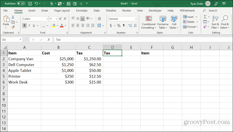
12. Paste Multiples of a Single Cell

If you have a single cell of data that you want to replicate over many cells, you can copy the individual cell and paste it over as many cells as you like. Select the cell you want to copy and press Control+C to copy.

Then choose any range of cells where you want to copy the data.

This will replicate that cell across as many cells as you like.

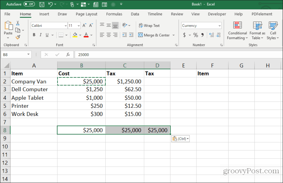
13. Copy Column Width

When copying and pasting a column of cells and you want the destination to be the same width as the original, there’s a trick to that as well.

Just copy the original column of cells as you normally would using the Control-C keys. Right-click the first cell in the destination and press Control-V to paste.

Now, select the original column of cells again and press Control-C. Right-click the first cell in the column you previously pasted and choose Paste Special.

In the Paste Special window, enable Column widths and select OK.

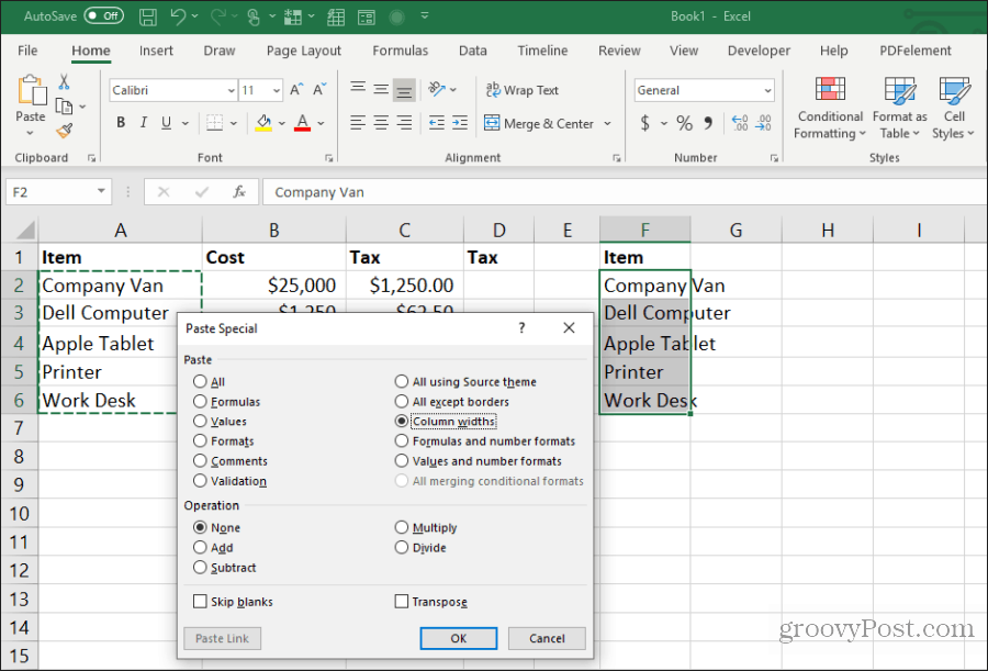
This will automatically adjust the column width to match the original widths as well.

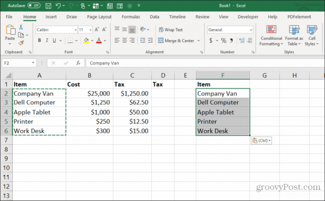
It might be easier to adjust the column width with your mouse, but if you’re adjusting the width of multiple columns at once on a huge sheet, this trick will save you a lot of time.

14. Paste with Calculation

Have you ever wanted to copy a number to a new cell but perform a calculation on it simultaneously? Most people will copy the number to a new cell and then type a formula to perform the calculation.

You can save that extra step by performing the calculation during the paste process.

Starting with a sheet containing the numbers you want to calculate, first select all of the original cells and press Control+C to copy. Paste those cells into the destination column where you want the results.

Next, select the second range of cells you want to calculate and press Control+C to copy. Select the destination range again, right-click, and choose Paste Special.

In the Paste Special window, under Operation, select the operation you want to perform on the two numbers. Select OK, and the results will appear in the destination cells.

This is a fast and easy way to perform quick calculations in a spreadsheet without using extra cells to do quick calculations.

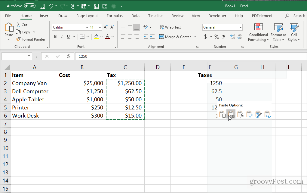
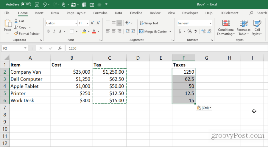
15. Transpose Column to Row

The most useful paste trick of all is transposing a column into a row. This is especially useful when you have one sheet with items vertically along a column that you want to use as headers in a new sheet.

First, highlight and copy (using Control+C) the column of cells you want to transpose as a row in your new sheet.

Switch to a new sheet and select the first cell. Right-click and select the transpose icon under Paste Options.

This pastes the original column into the new sheet as a row.

It’s fast and easy and saves the trouble of copying and pasting all of the individual cells.

Use all of the 15 tips and tricks above to save yourself a lot of time the next time you’re working with your Excel worksheets.

Источник

While working in Excel, we often copy values or formulas from other worksheets, from other programs or even from the web. For every copied value, we have specific preferences like copying without formatting, copying only the values or only the formulas. It becomes troublesome if the copied values distort the current format in our worksheets.

The Paste Special feature offers a variety of ways to copy and paste values according to our needs.

Figure 1. Final result: Copy without formatting

How to copy and paste without changing the format

In order to copy values or formula without changing the format, we launch the Paste Special tool in Excel.

To copy: Press Ctrl + C to copy cells with values, text or formula

To paste: Click Home tab > Paste > Paste Special

Figure 2. Paste Special feature

The Paste Special dialog box offers customized ways to paste the copied data. With this tool, we are able to copy only the values, formulas, format or any combination with number formats.

Figure 3. Excel Paste Special dialog box

Copy values without formatting

When we simply employ the Ctrl + C and Ctrl + V shortcuts to copy and paste values, we might end up with a table with varying formats such as this:

Figure 4. Copy values including formatting

In order to copy selected values while keeping the destination formatting, we follow these steps:

Copy the selected value

Figure 5. Copying the source cell

Select the cell where we want to paste the value

Figure 6. Selecting the destination cell

Click Home tab > Paste > Paste Special > Paste Values button

Figure 7. Paste Values button in Paste options

The name “Ann Taylor” will be copied without formatting, all the while keeping the destination cell formatting.

Figure 8. Output: Copy values without formatting

Copy formula without formatting

When we copy a formula in one cell and paste it on another cell, we are at risk of also copying the format of the source cell. In below example, we want to copy the formula for age in cell D3.

Formula: =NOW()-C3/365.

Figure 9. Example: copy exact formula for age

When we simply paste the formula in cell D4 through the shortcut Ctrl + V or the menu options, we also copy the red text color format into cell D4.

Figure 10. Pasting the copied formula with format into destination cell

We want to copy the formula exactly as it is in the cell, without the formatting.

Work-around:

Copy cell D3
Select cell D4
Click Home tab > Paste > Paste Special
In the Paste Special dialog box, tick the Formulas radio button

Only the formula is copied, keeping the blue text color format of cell D4.

Figure 11. Output: Copy exact formula

Copy values not formula

This time let us learn how to copy numbers without the formula. Suppose we want to copy the age from a separate database in another worksheet.

Copy cell D3

Figure 12. Copying the age from source cell

When we paste the copied cell into the destination cell, we have copied the formula as well.

Figure 13. Pasting the copied cell with formula

Work-around:

When we want to copy only the value and not the formula, we follow these steps.

Select the source cell and press Ctrl + C
Select the destination cell
Click Home tab > Paste > Paste Special
In the Paste Special dialog box, tick the Values radio button

Finally, we are able to copy the value and not the formula, as shown in cell E9.

Figure 14. Output: Copy values not formulas

Instant Connection to an Excel Expert

Most of the time, the problem you will need to solve will be more complex than a simple application of a formula or function. If you want to save hours of research and frustration, try our live Excelchat service! Our Excel Experts are available 24/7 to answer any Excel question you may have. We guarantee a connection within 30 seconds and a customized solution within 20 minutes.

Источник

Move or copy cells and cell contents

Need more help?

See Also

Need more help?

Want more options?

Copy and Paste Formulas in Excel without Changing Cell References

Manually Copy Paste the Exact Formula

Using Find and Replace

Using Notepad to Copy Paste Formulas

Get 51 Excel Tips Ebook to skyrocket your productivity and get work done faster

31 thoughts on “How to Copy and Paste Formulas in Excel without Changing Cell References”

References

About This Article

Is this article up to date?

1. Copy Formula Results

2. Copy Formulas Without Changing References

3. Avoid Copying Hidden Cells

4. Fill to Bottom with Formula

5. Copy Using Drag and Drop

6. Copy from Cell Above

7. Copy from Left Cell

8. Copy Cell Formatting

9. Copy Entire Sheet

10. Repeat Fill

11. Paste Entire Blank Column or Row

12. Paste Multiples of a Single Cell

13. Copy Column Width

14. Paste with Calculation

15. Transpose Column to Row

How to copy and paste without changing the format

Copy values without formatting

Copy formula without formatting

Copy values not formula

Work-around:

Instant Connection to an Excel Expert