
Excel 2013 Office for business Spreadsheet Compare 2013 Spreadsheet Compare 2016 Spreadsheet Compare 2019 Spreadsheet Compare 2021 More…Less
Let’s say you have two Excel workbooks, or maybe two versions of the same workbook, that you want to compare. Or maybe you want to find potential problems, like manually-entered (instead of calculated) totals, or broken formulas. You can use Microsoft Spreadsheet Compare to run a report on the differences and problems it finds.
Important: Spreadsheet Compare is only available with Office Professional Plus 2013, Office Professional Plus 2016, Office Professional Plus 2019, or Microsoft 365 Apps for enterprise.
Open Spreadsheet Compare
On the Start screen, click Spreadsheet Compare. If you do not see a Spreadsheet Compare option, begin typing the words Spreadsheet Compare, and then select its option.
In addition to Spreadsheet Compare, you’ll also find the companion program for Access – Microsoft Database Compare. It also requires Office Professional Plus versions or Microsoft 365 Apps for enterprise.
Compare two Excel workbooks
-
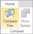
Click Home > Compare Files.

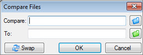
The Compare Files dialog box appears.
-
Click the blue folder icon next to the Compare box to browse to the location of the earlier version of your workbook. In addition to files saved on your computer or on a network, you can enter a web address to a site where your workbooks are saved.
-
Click the green folder icon next to the To box to browse to the location of the workbook that you want to compare to the earlier version, and then click OK.
Tip: You can compare two files with the same name if they’re saved in different folders.
-
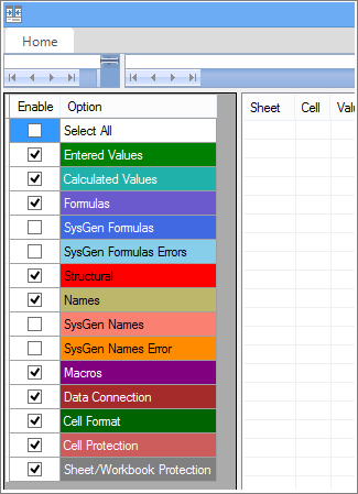
In the left pane, choose the options you want to see in the results of the workbook comparison by checking or unchecking the options, such as Formulas, Macros, or Cell Format. Or, just Select All.
-
Click OK to run the comparison.
If you get an «Unable to open workbook» message, this might mean one of the workbooks is password protected. Click OK and then enter the workbook’s password. Learn more about how passwords and Spreadsheet Compare work together.
The results of the comparison appear in a two-pane grid. The workbook on the left corresponds to the «Compare» (typically older) file you chose and the workbook on the right corresponds to the «To» (typically newer) file. Details appear in a pane below the two grids. Changes are highlighted by color, depending on the kind of change.
Understanding the results
-
In the side-by-side grid, a worksheet for each file is compared to the worksheet in the other file. If there are multiple worksheets, they’re available by clicking the forward and back buttons on the horizontal scroll bar.
Note: Even if a worksheet is hidden, it’s still compared and shown in the results.
-
Differences are highlighted with a cell fill color or text font color, depending on the type of difference. For example, cells with «entered values» (non-formula cells) are formatted with a green fill color in the side-by-side grid, and with a green font in the pane results list. The lower-left pane is a legend that shows what the colors mean.
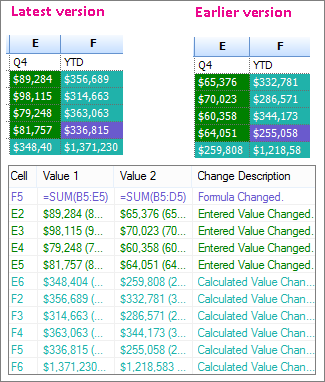
In the example shown here, results for Q4 in the earlier version weren’t final. The latest version of the workbook contains the final numbers in the E column for Q4.
In the comparison results, cells E2:E5 in both versions have a green fill that means an entered value has changed. Because those values changed, the calculated results in the YTD column also changed – cells F2:F4 and E6:F6 have a blue-green fill that means the calculated value changed.
The calculated result in cell F5 also changed, but the more important reason is that in the earlier version its formula was incorrect (it summed only B5:D5, omitting the value for Q4). When the workbook was updated, the formula in F5 was corrected so that it’s now =SUM(B5:E5).
-
If the cells are too narrow to show the cell contents, click Resize Cells to Fit.
Excel’s Inquire add-in
In addition to the comparison features of Spreadsheet Compare, Excel 2013 has an Inquire add-in you can turn on that makes an «Inquire» tab available. From the Inquire tab, you can analyze a workbook, see relationships between cells, worksheets, and other workbooks, and clean excess formatting from a worksheet. If you have two workbooks open in Excel that you want to compare, you can run Spreadsheet Compare by using the Compare Files command.
If you don’t see the Inquire tab in Excel, see Turn on the Inquire add-in. To learn more about the tools in the Inquire add-in, see What you can do with Spreadsheet Inquire.
Next steps
If you have «mission critical» Excel workbooks or Access databases in your organization, consider installing Microsoft’s spreadsheet and database management tools. Microsoft Audit and Control Management Server provides powerful change management features for Excel and Access files, and is complemented by Microsoft Discovery and Risk Assessment Server, which provides inventory and analysis features, all aimed at helping you reduce the risk associated with using tools developed by end users in Excel and Access.
Also see Overview of Spreadsheet Compare.
Need more help?
Want more options?
Explore subscription benefits, browse training courses, learn how to secure your device, and more.
Communities help you ask and answer questions, give feedback, and hear from experts with rich knowledge.
-
1
Highlight the first cell of a blank column. When comparing two columns in a worksheet, you’ll be outputting your results onto a blank column. Make sure you are starting on the same row as the two columns you’re comparing.
- For example, if the two columns you want to compare start on A2 and B2, highlight C2.
-
2
Type the comparison formula for the first row. Type the following formula, which will compare A2 and B2. Change the cell values if your columns start on different cells:
- =IF(A2=B2,"Match","No match")
Advertisement
-
3
Double-click the Fill box in the bottom corner of the cell. This will apply the formula to the rest of the cells in the column, automatically adjusting the values to match.
-
4
Look for Match and No match. These will indicate whether the contents of the two cells had matching data. This will work for strings, dates, numbers, and times. Note that case is not taken into consideration («RED» and «red» will match).[1]


Advertisement
-
1
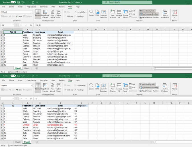
Open the first workbook you want to compare. You can use the View Side by Side feature in Excel to view two different Excel files on the screen at the same time. This has the added benefit of scrolling both sheets at once.
-
2
Open the second workbook. You should now have two instances of Excel open on your computer.
-
3
Click the View tab on either window.
-
4
Click View Side by Side. You’ll find this in the Window section of the ribbon. Both workbooks will appear in on the screen, oriented horizontally.
-
5
Click Arrange All to change the orientation.
-
6
Click Vertical and then OK. The workbooks will change so that one is on the left and the other is on the right.
-
7
Scroll in one window to scroll in both. When Side by Side is enabled, scrolling will be synchronized between both windows. This will allow you to easily look for differences as you scroll through the spreadsheets.
- You can disable this feature by clicking the Synchronous Scrolling button in the View tab.


Advertisement
-
1
Open the workbook containing the two sheets you want to compare. To use this comparison formula, both sheets must be in the same workbook file.
-
2
Click the + button to create a new blank sheet. You’ll see this at the bottom of the screen to the right of your open sheets.
-
3
Place your cursor in cell A1 on the new sheet.
-
4
Enter the comparison formula. Type or copy the following formula into A1 on your new sheet:
- =IF(Sheet1!A1<> Sheet2!A1, "Sheet1:"&Sheet1!A1&" vs Sheet2:"&Sheet2!A1, "")
-
5
Click and drag the Fill box in the corner of the cell.
-
6
Drag the Fill box down. Drag it down as far down as the first two sheets go. For example, if your spreadsheets go down to Row 27, drag the Fill box down to that row.
-
7
Drag the Fill box right. After dragging it down, drag it to the right to cover the original sheets. For example, if your spreadsheets go to Column Q, drag the Fill box to that column.
-
8
Look for differences in the cells that don’t match. After dragging the Fill box across the new sheet, you’ll see cells fill wherever differences between the sheets were found. The cell will display the value of the cell in the first sheet and the value of the same cell in the second sheet.
- For example, A1 in Sheet1 is «Apples,» and A1 in Sheet2 is «Oranges.» A1 in Sheet3 will display «Sheet1:Apples vs Sheet2:Oranges» when using this comparison formula.[2]
- For example, A1 in Sheet1 is «Apples,» and A1 in Sheet2 is «Oranges.» A1 in Sheet3 will display «Sheet1:Apples vs Sheet2:Oranges» when using this comparison formula.[2]


Advertisement
Add New Question
-
Question
How do I find duplicate values in a row?

To find duplicate values simply use the Data —> Remove Duplicates feature and follow the prompts on the screen.
-
Question
How do I subtract two rows?
You have to select the 2 rows {shift} and then right click on the now highlighted rows. A box will pop up with a list of actions. You should click on ‘delete rows’.
Ask a Question
200 characters left
Include your email address to get a message when this question is answered.
Submit
Advertisement
Thanks for submitting a tip for review!
About This Article
Article SummaryX
1. Highlight the first cell in a blank column.
2. Type » =IF(A2=B2,»Match»,»No match»)».
3. Drag the formula down to populate all cells in the column.
4. Look for «Match» or «No match» in the results.
Did this summary help you?
Thanks to all authors for creating a page that has been read 1,832,430 times.
Is this article up to date?
Watch Video – How to Compare Two Excel Sheets for Differences
Comparing two Excel files (or comparing two sheets in the same file) can be tricky as an Excel workbook only shows one sheet at a time.
This becomes more difficult and error-prone when you have a lot of data that needs to be compared.
Thankfully, there are some cool features in Excel that allow you to open and easily compare two Excel files.
In this Excel tutorial, I will show you multiple ways to compare two different Excel files (or sheets) and check for differences. The method you choose will depend on how your data is structured and what kind of comparison you’re looking for.
Let’s get started!
Compare Two Excel Sheets in Separate Excel Files (Side-by-Side)
If you want to compare two separate Excel files side by side (or two sheets in the same workbook), there is an in-built feature in Excel to do this.
It’s the View Side by Side option.
This is recommended only when you have a small dataset and manually comparing these files is likely to be less time-consuming and error-prone. If you have a large dataset, I recommend using the conditional method or the formula method covered later in this tutorial.
Let’s see how to use this when you have to compare two separate files or two sheets in the same file.
Suppose you have two files for two different months and you want to check what values are different in these two files.
By default, when you open a file, it’s likely to take up your entire screen. Even if you reduce the size, you always see one Excel file at the top.
With the view side-by-side option, you can open two files and then arrange these horizontally or vertically. This allows you to easily compare the values without switching back and forth.
Below are the steps to align two files side by side and compare them:
- Open the files that you want to compare.
- In each file, select the sheet that you want to compare.
- Click the View tab

- In the Windows group, click on the ‘View Side by Side’ option. This becomes available only when you have two or more Excel files open.


As soon as you click on the View side by side option, Excel will arrange the workbook horizontally. Both of the files will be visible, and you’re free to edit/compare these files while they are arranged side by side.

In case you want to arrange the files vertically, click on the Arrange All option (in the View tab).

This will open the ‘Arrange Windows’ dialog box where you can select ‘Vertical’.

At this point, if you scroll down in one of the worksheets, the other one would remain as is. You can change this so that when you scroll in one sheet, the other also scrolls at the same time. This makes it easier to do a line by line comparison and spot any differences.
But to do this, you need to enable Synchronous Scrolling.
To enable Synchronous Scrolling, click on the View tab (in any of the workbooks) and then click on the Synchronous Scrolling option. This is a toggle button (so if you want to turn it off, simply click on it again).

Comparing Multiple Sheets in Separate Excel Files (Side-by-Side)
With the ‘View Side by Side’ option, you can only compare two Excel file at one go.
In case you have multiple Excel files open, when you click on the View Side by Side option, it will show you a ‘Compare Side by Side’ dialog box, where you can choose which file you want to compare with the active workbook.
In case you want to compare more than two files at one go, open all these files and then click on the Arrange All option (it’s in the View tab).
In the Arrange Windows dialog box, select Vertical/Horizontal and then click OK.
This will arrange all the open Excel files in the selected order (vertical or horizontal).
Compare Two Sheets (Side-by-Side) in the Same Excel Workbook
In case you want to compare two separate sheets in the same workbook, you can’t use the View side by side feature (as it works for separate Excel files only).
But you can still do the same side-by-side comparison.
This is made possible by the ‘New Windows’ feature in Excel, that allows you to open two instances on the same workbook. Once you have two instances open, you can arrange these side by side and then compare these.
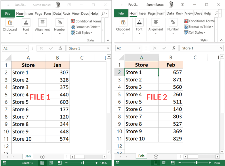
Suppose you have an Excel workbook that has two sheets for two different months (Jan and Feb) and you want to compare these side by side to see how the sales per store have changed:

Below are the steps to compare two sheets in Excel:
- Open the workbook that has the sheets that you want to compare.
- Click the View tab
- In the Window group, click on the ‘New Window’ option. This opens the second instance of the same workbook.
- In the ‘View’ tab, click on ‘Arrange All’. This will open the Arrange Windows dialog box

- Select ‘Vertical’ to compare data in columns (or select Horizontal if you want to compare data in rows).

- Click OK.
The above steps would arrange both the instances of the workbook vertically.
At this point in time, both the workbooks would have the same worksheet selected. In one of the workbooks, select the other sheet that you want to compare with the active sheet.
How does this work?
When you click on New Window, it opens the same workbook again with a slightly different name. For example, if your workbook name is ‘Test’ and you click on New Window, it will name the already open workbook ‘Test – 1’ and the second instance as ‘Test – 2’.
Note that these are still the same workbook. If you make any changes in any of these workbooks, it would be reflected in both.
And when you close any one instance of the open file, the name would revert back to the original.
You can also enable synchronous scrolling if you want (by clicking on the ‘Synchronous Scrolling’ option in the ‘View’ tab)
Compare Two Sheets and Highlight Differences (Using Conditional Formatting)
While you can use the above method to align the workbooks together and manually go through the data line by line, it’s not a good way in case you have a lot of data.
Also, doing this level of comparison manually can lead to a lot of errors.
So instead of doing this manually, you can use the power of Conditional Formatting to quickly highlight any differences in the two Excel sheets.
This method is really useful if you have two versions in two different sheets and you want to quickly check what has changed.
Note that you CAN NOT compare two sheets in different workbooks.
Since Conditional Formatting can not refer to an external Excel file, the sheets you need to compare needs to be in the same Excel workbook. In case these aren’t, you can copy a sheet from the other file to the active workbook and then make this comparison.
For this example, suppose you have a dataset as shown below for two months (Jan and Feb) in two different sheets and you want to quickly compare the data in these two sheets and check if the prices of these items have changed or not.

Below are the steps to do this:
- Select the data in the sheet where you want to highlight the changes. Since I want to check how prices have changed from Jan to Feb, I have selected the data in the Feb sheet.
- Click the Home tab

- In the Styles group, click on ‘Conditional Formatting’

- In the options that show up, click on ‘New Rule’

- In the ‘New Formatting Rule’ dialog box, click on ‘Use a formula to determine which cells to format’

- In the formula field, enter the following formula: =B2<>Jan!B2
- Click the Format button
- In the Format Cells dialog box that shows up, click on the ‘Fill tab’ and select the color in which you want to highlight the mismatched data.

- Click OK
- Click OK


The above steps would instantly highlight any changes in the dataset in both the sheets.

How does this work?
Conditional formatting highlights a cell when the given formula for that cell returns a TRUE. In this example, we are comparing each cell in one sheet with the corresponding cell in the other sheet (done using the not equal to operator <> in the formula).
When conditional formatting finds any difference in the data, it highlights that in the Jan sheet (the one in which we have applied the conditional formatting.
Note that I have used relative reference in this example (A1 and not $A$1 or $A1 or A$1).
When using this method to compare two sheets in Excel, remember the following;
- This method is good to quickly identify differences, but you can’t use it on an on-going basis. For example, if I enter a new row in any of the datasets (or delete a row), it would give me incorrect results. As soon as I insert/delete the row, all subsequent rows are considered as different and highlighted accordingly.
- You can only compare two sheets in the same Excel file
- You can only compare the value (not the difference in formula or formatting).
Compare Two Excel Files/Sheets And Get The Differences Using Formula
If you’re only interested in quickly comparing and identifying the differences between two sheets, you can use a formula to fetch only those values that are different.
For this method, you will need to have a separate worksheet where you can fetch the differences.
This method would work if want to compare two separate Excel workbook or worksheets in the same workbook.
Let me show you an example where I am comparing two datasets in two sheets (in the same workbook).
Suppose you have the dataset as shown below in a sheet called Jan (and similar data in a sheet called Feb), and you want to know what values are different.
To compare the two sheets, first, insert a new worksheet (let’s call this sheet ‘Difference’).
In cell A1, enter the following formula:
=IF(Jan!A1<>Feb!A1,"Jan Value:"&Jan!A1&CHAR(10)&"Feb Value:"&Feb!A1,"")

Copy and paste this formula for a range so that it covers the entire dataset in both the sheets. Since I have a small dataset, I will only copy and paste this formula in A1:B10 range.
The above formula uses an IF condition to check for differences. In case there is no difference in the values, it will return blank, and in case there is a difference, it will return the values from both the sheets in separate lines in the same cell.
The good thing with this method is that it only gives you the differences and show you exactly what the difference is. In this example, I can easily see that the price in cell B4 and B8 are different (as well as the exact values in these cells).
Compare Two Excel Files/Sheets And Get The Differences Using VBA
If you need to compare Excel files or sheets quite often, it’s a good idea to have a ready Excel macro VBA code and use it whenever you need to make the comparison.
You can also add the macro to the Quick Access Toolbar so that you can access with a single button and instantly know what cells are different in different files/sheets.
Suppose you have two sheets Jan and Feb and you want to compare and highlight differences in the Jan sheet, you can use the below VBA code:
Sub CompareSheets()
Dim rngCell As Range

For Each rngCell In Worksheets("Jan").UsedRange

    If Not rngCell = Worksheets("Feb").Cells(rngCell.Row, rngCell.Column) Then
        rngCell.Interior.Color = vbYellow
    End If

Next rngCell

End Sub
The above code uses the For Next loop to go through each cell in the Jan sheet (the entire used range) and compares it with the corresponding cell in the Feb sheet. In case it finds a difference (which is checked using the If-Then statement), it highlights those cells in yellow.
You can use this code in a regular module in the VB Editor.
And if you need to do this often, it’s better to save this code in the Personal Macro workbook and then add it to the Quick Access toolbar. In those ways, you will be able to do this comparison with a click of a button.
Here are the steps to get the Personal Macro Workbook in Excel (it’s not available by default so you need to enable it).
Here are the steps to save this code in the Personal Macro Workbook.
And here you will find the steps to add this macro code to the QAT.
Using a Third-Party Tool – XL Comparator
Another quick way to compare two Excel files and check for matches and differences is by using a free third-party tool such as XL Comparator.
This is a web-based tool where you can upload two Excel files and it will create a comparison file that will have the data that is common (or different data based on what option you selected.
Suppose you have two files that have customer datasets (such as name and email address), and you want to quickly check what customers are there is file 1 and not in file 2.
Below is how you compare two Excel files and create a comparison report:
- Open https://www.xlcomparator.net/
- Use the Choose file option to upload two files (maximum size of each file can be 5MB)
- Click on the Next button.
- Select the common column in both these files. The tool will use this common column to look for matches and differences
- Select one of the four options, whether you want to get matching data or different data (based on File 1 or File 2)
- Click on Next
- Download the comparison file which will have the data (based on what option you selected in step 5)
Below is a video that shows how XL Comparator tool works.
One concern you may have when using a third-party tool to compare Excel files is about privacy.
If you have confidential data and privacy is really important for it, it’s better to use other methods shown above.
Note that the XL Comparator website mentions that they delete all the files after 1 hour of doing the comparison.
These are some of the methods you can use to compare two different Excel files (or worksheets in the same Excel file). Hope you found this Excel tutorial useful.
You may also like the following Excel tutorials:
- How to Compare Two Columns in Excel (for matches & differences)
- How to Remove Duplicates in Excel
- How to Compare Text in Excel (Easy Formulas)
- Split Each Excel Sheet Into Separate Files (Step-by-Step)
- Combine Data from Multiple Workbooks in Excel
- Combine Data From Multiple Worksheets into a Single Worksheet in Excel
- How to Compare Dates in Excel (Greater/Less Than, Mismatches)
How to Compare Two Lists in Excel? (Top 6 Methods)
Below are the six different methods used to compare two lists of a column in Excel for matches and differences.
- Method 1: Compare Two Lists Using Equal Sign Operator
- Method 2: Match Data by Using the Row Difference Technique
- Method 3: Match Row Difference by Using the IF Condition
- Method 4: Match Data Even If There is a Row Difference
- Method 5: Highlight All the Matching Data using Conditional Formatting
- Method 6: Partial Matching Technique
Table of contents
- How to Compare Two Lists in Excel? (Top 6 Methods)
- #1 Compare Two Lists Using Equal Sign Operator
- #2 Match Data by Using Row Difference Technique
- #3 Match Row Difference by Using IF Condition
- #4 Match Data Even If There is a Row Difference
- #5 Highlight All the Matching Data
- #6 Partial Matching Technique
- Things to Remember
- Recommended Articles
Now, let us discuss each of the methods in detail with an example: –
You can download this Compare Two Lists Excel Template here – Compare Two Lists Excel Template
#1 Compare Two Lists Using Equal Sign Operator
We must follow the below steps to compare the two lists.
- Immediately after the two columns, we must insert a new column called “Status” in the next column.

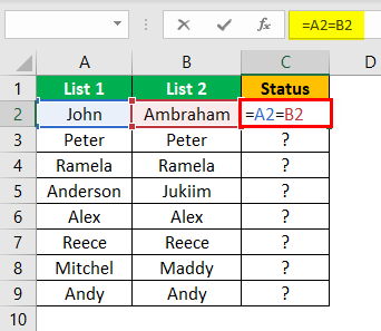
- Now, we must put the formula in cell C2 as =A2=B2.

- This formula tests whether the cell A2 value is equal to cell B2. If both cell values are matched, we will get TRUE or FALSE results.

- We will drag the formula to cell C9 to determine the other values.


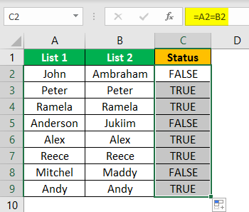
Wherever we have the same values in common rows, we get the result as “TRUE” or “FALSE.”
#2 Match Data by Using Row Difference Technique
You might not have used the “Row Difference” technique at your workplace. But today, we will show you how to use this technique to match data row by row.
- Step 1: To highlight non-matching cells row by row, we must select the entire data first.

- Step 2: Now, we must press the excel shortcut keyAn Excel shortcut is a technique of performing a manual task in a quicker way.read more “F5” to open the “Go to Special” tool.
![]()
- Step 3: Press the “F5” key to open this window. In the “Go To” window, press the “Special” tab.

- Step 4: In the next window, we must go to the “Go To Special” and choose the “Row differences” option. Then, click on “OK.”

We will get the following result.

As shown in the above window, it has selected the cells wherever there is a row difference. Therefore, we must fill in some colors to highlight the row difference values.

#3 Match Row Difference by Using IF Condition
How can we leave out the IF condition when we want to match data row by row? In the first example, we have either “TRUE” or “FALSE.” But what if we need a different result instead of the default results of either “TRUE or FALSE.” Assume we need a result as “Matching” if there is no row difference, and the result should be “Not Matching” if there is a row difference.
- Step 1: First, we must open the IF condition in cell C2.

- Step 2: Then, apply the logical testA logical test in Excel results in an analytical output, either true or false. The equals to operator, “=,” is the most commonly used logical test.read more as A2=B2.
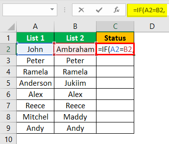
- Step 3: We must enter the result criteria if the logical test is “TRUE.” In this scenario, the result criteria are “Matching,” If the row does not match, we need the result as “Not Matching.”

- Step 4: Next, we need to apply the formula to get the result.
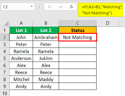
- Step 5: We must drag the formula to cell C9 to determine the other values.

#4 Match Data Even If There is a Row Difference
The matching data on the row differences method may not always work; the value may be in other cells too. So we need to use different technologies in these scenarios.
Now, look at the below data.

In the above image, we have two lists of numbers. We need to compare list 2 wish list 1. So let us use our favorite function VLOOKUPThe VLOOKUP excel function searches for a particular value and returns a corresponding match based on a unique identifier. A unique identifier is uniquely associated with all the records of the database. For instance, employee ID, student roll number, customer contact number, seller email address, etc., are unique identifiers.
read more.

So, if the data matches, we get the number; otherwise, we get the error value as #N/A.
Showing error values does not look good. So instead of showing the error, let us replace them with the word “Not Available.” For this, use the IFERROR function in ExcelThe IFERROR function in Excel checks a formula (or a cell) for errors and returns a specified value in place of the error.read more.

#5 Highlight All the Matching Data
If you are not a fan of Excel formulasThe term «basic excel formula» refers to the general functions used in Microsoft Excel to do simple calculations such as addition, average, and comparison. SUM, COUNT, COUNTA, COUNTBLANK, AVERAGE, MIN Excel, MAX Excel, LEN Excel, TRIM Excel, IF Excel are the top ten excel formulas and functions.read more, do not worry. We can still match data without the formula. For example, using simple conditional formatting in ExcelConditional formatting is a technique in Excel that allows us to format cells in a worksheet based on certain conditions. It can be found in the styles section of the Home tab.read more, we can highlight all the matching data of two lists.
- Step 1: We must first select the data.

- Step 2: Now, we must go to “Conditional Formatting” and choose “Highlight Cell Rules” >> “Duplicate Values.”

- Step 3: As a result, we can see the “Duplicate Cell Values” formatting window.

- Step 4: We can choose the different formatting colors from the drop-down list in ExcelA drop-down list in excel is a pre-defined list of inputs that allows users to select an option.read more. Select the first formatting color and press the “OK” button.

- Step 5: This will highlight all the matching data from the two lists.

- Step 6: Just in case, instead of highlighting all the matching data, if we want to highlight not matching data, then we can go to the “Duplicate Values” window and choose the option “Unique.”

As a result, it will highlight all the non-matching values, as shown below.

#6 Partial Matching Technique
We have seen the issue of not having full or the same data in two lists. For example, if the List 1 data has “ABC Pvt Ltd.“ In List 2, we have “ABC” only. In these cases, all our default formulas and tools are not recognized. Therefore, we need to employ the special character asterisk (*) to match partial values in these cases.

In List 1, we have the company name and revenue details. In List 2, we have company names but not exact values as in List 1. It is a tricky situation that we all have faced at our workplace.
In such cases, still, we can match data by using a special character asterisk (*).

We get the following result.

We will drag the formula to cell E9 to determine the other values.

The wildcard character asterisk (*) was used to represent any number of characters so that it will match the full character for the word “ABC” as “ABC Pvt Ltd.”
Things to Remember
- The use of the above techniques for comparing two lists in Excel upon the data structure.
- If the data is not organized, row-by-row matching is not the best suited.
- VLOOKUP is the often-used formula to match values.
Recommended Articles
This article is a guide to Compare Two Lists in Excel. We discuss the top 6 methods to compare two columns list in Excel for the match, along with examples and a downloadable Excel template. You may learn more about Excel from the following articles: –
- Compare Two Excel Columns Using Vlookup
- Partial Match with Vlookup
- Compare Two Excel Columns
- Shade Alternate Rows in Excel
One of the most common scenarios when working with Excel spreadsheets is having files with similar or duplicate data. The reasons for this could be many, but it usually involves spending a considerable amount of time checking complete files or separate worksheets manually.
This article will explain how to compare two or multiple Excel files, as well as two Excel sheets, for differences. To achieve this, we will describe how to use three useful methods to spot differences in a quick and easy way; these include side-by-side viewing, conditional formatting rules, and the =IF formula.
How to compare two Excel files using side-by-side view?
We will start by illustrating how to compare two Excel workbooks using the side-by-side view. However, we recommend using this method in case your dataset is not too large; if not, we recommend using one of the two methods outlined further on in this article. This is how you can compare two Excel files using the side-by-side viewing feature.
- 1. Open the two Excel workbooks you would like to compare and go to View > View Side by Side on any of the opened files.

How to compare two Excel files — View side by side
- 2. By default, Excel will place both files horizontally, as shown below.

How to compare two Excel files — Horizontal view
- 3. To arrange them vertically, click “Arrange All”, and then select “Vertical”.
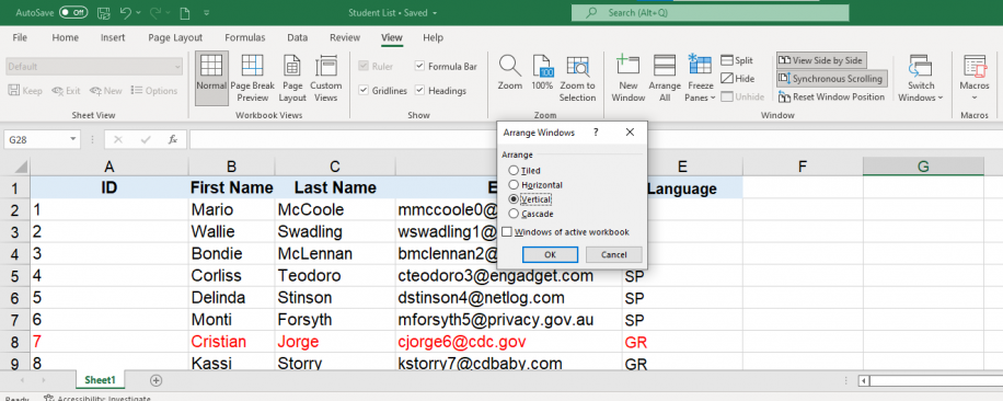
How to compare two Excel files — Arrange vertically
- 4. The two Excel files will now be arranged vertically, as shown below.

How to compare two Excel files — Vertical view
- 5. Make sure that the “Synchronous Scrolling” option is activated since this will allow you to scroll through the data on both files simultaneously and allow you to compare more easily. Although it activates automatically as soon as you enable the side-by-side view, you can also check that it’s activated in your toolbar within the “Window” group.
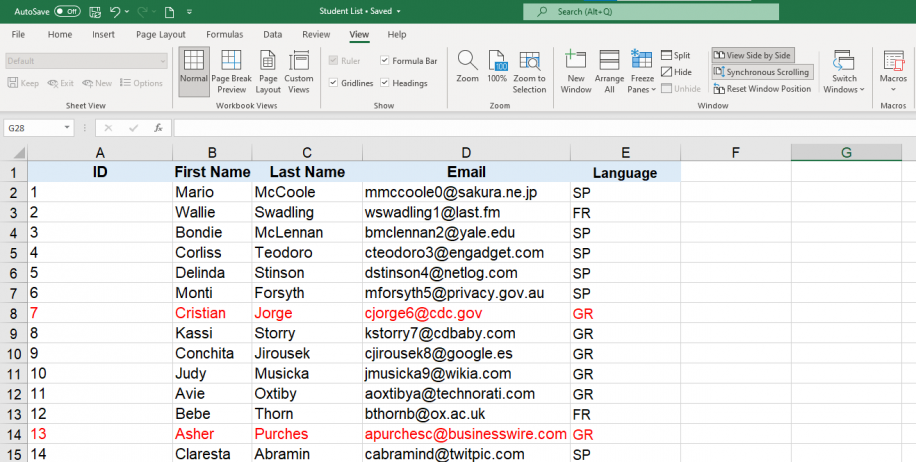
How to compare two Excel files — Synchronous Scrolling
Now that we know how easy it is to compare two Excel files, let’s see how we can apply this viewing method to Excel sheets.
How to Combine Multiple Excel Files Into One
Discover the most popular methods used to manually or automatically combine multiple Excel spreadsheets and data inputs into one master file
READ MORE

How to compare two Excel sheets using side-by-side view?
Sometimes, similar or duplicate data may appear within the same spreadsheet. IF you want to avoid having to switch from one sheet to another to compare the data, this is how you can quickly compare two Excel sheets side by side.
- 1. Open the Excel file where you would like to compare sheets. Then, go to View > New Window.

How to compare two Excel files — View New Window
- 2. You will now have the same Excel file open up in a different window, as shown below.

How to compare two Excel files — Same file in New Window
- 3. Select “View Side by Side” and make sure to select a different sheet on each file. As before, you can select vertical or horizontal viewing according to your preference.
How to compare two Excel files — Sheet 1 and 2
So far, you have seen how easy it is to compare two files and sheets on Excel. However, what if you would like to compare more than two files at the same time? This is how you can compare multiple Excel files using the side-by-side view.
How to compare multiple Excel files using side-by-side view?
Comparing multiple files for differences follows a similar process and will only take you a few simple steps.
- 1. Open all the Excel workbooks you would like to compare and go to View > View Side by Side. Select the file you want to start comparing with in the “Compare Side by Side” dialog box.

How to compare two Excel files — Compare side by side
- 2. Click “Arrange All” to view all the opened files at the same time.

How to compare two Excel files — Arrange All
- 3. Then, select the type of arrangement according to your preference. Here, I have chosen the “Tiled” arrangement.

How to compare two Excel files — Tiled arrangement
So far, these methods are useful in case your datasets are not too large and easily manageable. If you want to compare larger datasets for differences in values, the best way is to use the =IF formula or a conditional formatting rule. Let’s explore the =IF formula first.
How to compare two Excel sheets using a formula?
This is the most straightforward way to compare data between two Excel sheets. This formula will allow you to identify cells containing different values, and a comparative report will be generated in a new worksheet.
- 1. Open a new empty sheet in your Excel workbook and enter the following formula in cell A1: =IF(Sheet1!A1 <> Sheet2!A1, «Sheet1:»&Sheet1!A1&» vs Sheet2:»&Sheet2!A1, «»)

How to compare two Excel files — Enter IF formula
- 2. Grab the bottom-right corner of the formula cell, and drag down.

How to compare two Excel files — A1 cell comparison in Sheets
The formula will adapt to the column and row position it fills. This way, the formula in cell A1 compares to cell A1 in “Sheet1” and “Sheet2”; the formula in cell B1 will compare cell B1 in both sheets as well.
We will now turn to how to compare two Excel sheets by highlighting the differences. The best way to do so is by using the Excel conditional formatting feature.
How to compare two Excel sheets using conditional formatting?
When comparing two very similar and large datasets, the best and quickest way to spot differences in values is to highlight them using the conditional formatting feature.
- 1. Open the Excel sheets and select the range of data you would like to compare for differences. A quick way to do this is to click the upper-left cell and then Ctrl + Shift + End to extend the selection to the last cell containing values.

How to compare two Excel files — Select cell range
- 2. Go to Home > Conditional Formatting > New rule.

How to compare two Excel files — Create New Rule
- 3. Select the rule type “Use a formula to determine which cells to format” and enter the following, =A1<>Sheet1!A1. The Sheet name included in the formula corresponds to the sheet you are comparing with and not the one you are creating the rule in.

How to compare two Excel files — Use a formula
- 4. Once you’ve entered the formula, click “Format”, next to the “Preview” pane.

How to compare two Excel files — Format cells
- 5. Select how you would like to format the cells, i.e. according to “Number”, “Font”, “Border”, or “Fill”. We recommend highlighting with color fill, so we have chosen a color that will clearly stand out.

How to compare two Excel files — Format Fill
- 6. As you can see, Excel has highlighted the different cells in “Sheet 2” compared to “Sheet 1”.

How to compare two Excel files — Different cells highlighted
Now you know how to compare two or multiple Excel files and two sheets on your desktop. What if you want to compare and highlight differences in your Excel sheets online?
How to compare two Excel sheets and highlight differences online?
In case you don’t have Excel installed on your desktop or simply prefer to work online altogether, there are online tools that allow you to compare Excel files and sheets for differences.
Below, we provide a list of third-party tools that will allow you to compare Excel files and sheets online:
- Layer: Apart from allowing you to review spreadsheet changes and combine multiple spreadsheets into one, Layer offers additional features for file storage and management at a business level.
- Synkronizer Excel Compare: In addition to the features outlined in this article, it allows you to combine multiple Excel files into one, while maintaining unique values and avoiding duplicates.
- Ablebits Compare Sheets for Excel: This tool provides step-by-step guidance for efficient comparison and displays the differences found between sheets in the “Review Differences” mode for better management.
- Florencesoft DiffEngineX: Another excellent alternative that allows you to compare Excel files directly from Microsoft Outlook.
Want to Boost Your Team’s Productivity and Efficiency?
Transform the way your team collaborates with Confluence, a remote-friendly workspace designed to bring knowledge and collaboration together. Say goodbye to scattered information and disjointed communication, and embrace a platform that empowers your team to accomplish more, together.
Key Features and Benefits:
- Centralized Knowledge: Access your team’s collective wisdom with ease.
- Collaborative Workspace: Foster engagement with flexible project tools.
- Seamless Communication: Connect your entire organization effortlessly.
- Preserve Ideas: Capture insights without losing them in chats or notifications.
- Comprehensive Platform: Manage all content in one organized location.
- Open Teamwork: Empower employees to contribute, share, and grow.
- Superior Integrations: Sync with tools like Slack, Jira, Trello, and more.
Limited-Time Offer: Sign up for Confluence today and claim your forever-free plan, revolutionizing your team’s collaboration experience.
Conclusion
This article has shown you how to compare the data in two Excel files for differences. You can compare data between two files, two sheets, or multiple files using the side-by-side view for a quick and easy comparison. If your dataset is larger, you can apply the IF formula to compare two Excel sheets or use conditional formatting rules to highlight the differences.
Alternatively, for users that prefer to work online, there are platforms that can help you achieve this level of comparison in an online setting, for example, Layer. We also recommend reading our blog article on How To Combine Multiple Files into One as a great way to complete this data comparison process.
Hay Paula, can you compare lists in Excel?
or
What is the best way to compare two sets of data in Excel?
Very often there is a requirement in Excel to compare two lists, or two data sets to find missing or matching items. As this is Excel, there are always more than one way to do things, including comparing data. From formulas and Conditional Formatting to Power Query. In this article we are going to look at a number ways to compare two lists in Excel and we will also look at comparing entire rows of a data set.
Maybe your preferred way is not included below. If not why don’t you drop a comment below and share with us how you like to compare two lists or datasets in Excel. I look forward to reading your comments.
We wish to compare List 1 with List 2.

Contents
Quick Conditional Formatting to compare two columns of data
Clearing the Conditional Formatting
Match data in Excel using the MATCH function
Compare 2 lists in Excel 365 with MATCH or XMATCH as a Dynamic Array function
MATCH and Dynamic arrays to compare 2 lists
XMATCH Excel 365 to compare two lists
Tables – Comparing lists in Excel where the ranges sizes might change
Highlight differences in Lists using Custom Conditional Formatting
Copy formula to Custom Conditional Formatting
Other Formulas used to compare two lists in Excel
VLOOKUP to compare two lists in Excel
XLOOKUP to compare two lists in Excel
COUNTIF to compare two lists in Excel
How to compare 2 data sets in Excel
Comparing lists or datasets using Power Query

Quick Conditional Formatting to compare two columns of data
Conditional formatting will allow you to highlight a cells or range based on predefined criteria. The quickest and simplest way to visually compare these two columns quickly is to use the predefined highlight duplicate value rule.
Start by selecting the two columns of data.
From the Home tab, select the Conditional Formatting drop down. Then select Highlight Cells Rules. Next select Duplicate values.

A Duplicate Values settings box will open where you can define the formatting and select between Duplicate or Unique values.

By Selecting Duplicate, all reoccurring entries will be set to the selected formatting. Now you can quickly see the items in List 1 that are in List 2 as these are the formatted items. You can also quickly see the items in list 2 that are not in list 1 as these do not have formatting applied.

However, you can also format the Unique items. This can be achieved by selecting Unique from the Duplicate Values setup box.

In this case, we have applied two different conditional formats. The red indicating the duplicates and the green indicating the unique items.
Note, I did not just take the cells with data, I grabbed all of columns A to C. Column B has no data, so it cannot affect the results. However, these cells do contain the conditional formatting applied so it would be better practice to only select the cells you need.
Clearing the Conditional Formatting
To clear all conditional formatting, first select the cell, or range. Then select the conditional formatting drop down on the Home ribbon. Next select Clear Rules. Finally Select Clear Rules from Selected Cells.

If you have more than one conditional formatting applied at once and you only want to remove one of these, select Manage Rules from the conditional formatting drop down. Select the rule you want to delete and then select Delete Rule.

By pressing OK, the rule will removed from the Rules Manager and the cells will no longer contain the formatting.

So that is the most basic way you can compare two lists in Excel. Its quick, its simple and it is effective. You can also apply conditional formatting based on formulas, which we will look at later in this article.
Match data in Excel using the MATCH function
There are many lookup formulas that you can use to compare two ranges or lists in Excel. The first we will look at is the MATCH function.
The MATCH function returns the relative position in a list. A number based on its position, if found, in the lookup array.
The syntax for MATCH is
=MATCH (lookup value, Lookup array, Match type)
Where lookup value is the value you want to find a match for. Lookup array is the list in which you are looking for a match. And Match type allows you to select between an exact or approximate match.
We want to write a match formula to see if the items in List 2 are in List 1.
In cell E3 we can enter the formula
=MATCH(C2, $A$2:$A$21,0)

By filling this formula down, for the values where Excel finds a match, the position of that match will be returned. Where there is no match the return value will be an #N/A.

Very often, the relative position or the #N/A is of no value to us and we need to convert these values into true or false. To do this we can easily expand on our Match formula using a logical function. As Match returns a number, we can use the ISNUMBER function
=ISNUMBER(MATCH(C2, $A$2:$A$21,0))

Compare 2 lists in Excel 365 with MATCH or XMATCH as a Dynamic Array function
If you are using Excel 365 you have further alternatives when using MATCH to compare lists or data. As Excel 365 thinks in arrays, we can now pass an array as the lookup value of MATCH and our results will spill for us. This removes the need to copy the formula down and with only 1 formula, your spreadsheet will be less prone to errors and more compact.
MATCH and Dynamic arrays to compare 2 lists
If you are not yet familiar with Dynamic Arrays, I would suggest you have a read of this article: Excel Dynamic Arrays – A new way to model your Excel Spreadsheets: to get a better understand on how they work and spill ranges.
The only change to the match formula is instead of selecting cell C2 as our lookup value we will select the range C2:12
=ISNUMBER(MATCH (C2:C12,$A$2:$A$21,0))

As you can see, the one formula spills the results down column E.
XMATCH Excel 365 to compare two lists
Excel 365 also introduces the new function XMATCH. Just like the MATCH function XMATCH returns a relative position in a list. Now you are familiar XLOOKUP, which replaces the old VLOOKUP function, you know XLOOKUP comes with additional power. This come in the form of new conditions in the formula syntax such as search mode and match types. Well, XMATCH also as this extra power over its predecessor MATCH.
The syntax for XMATCH is
XMATCH (Lookup Value, Lookup Array, [Match Mode],[Search Mode])
Where
Lookup Value is the value you are looking to find the relative position
Lookup Array is the row or column that contains the Lookup Value
Match mode is optional. Unlike the old MATCH function, the default is an exact match. You can also select between
- Exact match or next smallest
- Exact match or next largest
- Wildcard match
Search mode is also optional. The default (and only option in the old MATCH function) is to look from the top down. You can also select last to first and binary searches. If you are working with binary searches. The wildcard match option does not work.
With XMATCH we can use either Dynamic arrays or cell references to create the formula, just like we have looked at with MATCH. For this example, we will use Dynamic Arrays. The formula is very similar to what we used with MATCH; except we do not have to select 0 for an exact match as in XMATCH this is the default setting. Let us mix things up a little this time a look at finding items in list 2 not in list one.
In this case we can use the formula
=NOT(ISNUMBER(XMATCH(C2:C12,A2:A21)))
Where not will turn trues into false and false into trues.

Tables – Comparing lists in Excel where the ranges sizes might change
In each of the formulas we have looked at so far, we have selected a range of cells in our Match functions that is not dynamic. That means if we add new data to one of the lists, we have a manual step to update our formula to include the new data.
To convert the lists to tables, select one of the lists and press CTRL. This is the keyboard shortcut to convert to a table. If you selected the header in the range of cells, ensure you tick the box to confirm your table has headers.

Tables by their nature use structured naming. Therefore, when you are writing a formula and you select a column from a table, it will not show cell references, but the column name.
Looking at our previous formula using XMATCH to find items in list 2 not in list 1, we can re-write this function now using our table references
=NOT (ISNUMBER(XMATCH(list2[List 2],list1[List 1])))

Now, as we have used tables, if we add a new row to either of the tables, our spill range will also increase to include the new data.

Highlight differences in Lists using Custom Conditional Formatting
Earlier in this article we looked at a very quick way of comparing these two lists using a predefined rule for duplicates. We can however also use Custom Conditional Formatting. If you are not familiar with Custom Conditional Formatting, I would suggest you check out this article: Excel Dynamic Conditional Formatting Tricks:
We need to look at two different approaches here to highlighting differences. When we are not using tables and we have created a true/false formula to identify the differences, we can take a copy of the formula and add this to our Custom formatting. However, with Tables we need to force the use of cell references.
Copy formula to Custom Conditional Formatting
Start by taking a copy of the formula. As we have tested the formula in the spreadsheet, we can see that it works before we use it in conditional formatting. This is best practice as very often with relative and absolute cell references it can be difficult to get the formula correct.

Select the cells that you want to apply the custom formatting to. Then from the Home ribbon select the conditional formatting drop down and select New Rule

The New Formatting Rule set up box will open and select Use Formula to determine which cells to format. Then paste in the formula and set the formatting type

This will result in all cells that are in both lists being formatted to your chosen format.

Keep in mind that we selected a range of cells to apply this conditional formatting and it is not dynamic. Should we use tables, this would update without the need to change anything!
Other Formulas used to compare two lists in Excel
There are many formulas you can use to compare two lists in Excel. We have already looked at MATCH and XMATCH, but now we are going to look at a few more. Any of the lookup functions will really work along with some others!
VLOOKUP to compare two lists in Excel
If you are not familiar with VLOOKUP, you can read about it here. Simply put VLOOKUP will return a corresponding value from a cell, if there is no corresponding value an #N/A error will be returned. In our example we are working with text. So, we can carry out a VLOOKUP and test to see if it returns text. If we were using numbers then we could replace ISTEXT with ISNUMBER.
We could use the function =ISTEXT(VLOOKUP(C2, $A$2:$A$21,1,FALSE))

Or if we were using Dynamic arrays in Excel 365, we could use the function
=ISTEXT(VLOOKUP (C2:C12,$A$2:$A$21,1,FALSE))

XLOOKUP to compare two lists in Excel
XLOOKUP was introduced in Excel 365 and you can find out more about it here. Very much like VLOOKUP, XLOOKUP will return a corresponding value from a cell, and you can define a result if the value is not found. Using Dynamic arrays, the function would be
=ISTEXT(XLOOKUP (C2:C12,A2:A21,A2:A21))

COUNTIF to compare two lists in Excel
The COUNTIF function will count the number of times a value, or text is contained within a range. If the value is not found, 0 is returned. We can combine this with an IF statement to return our true and false values.
=IF(COUNTIF (A2:A21,C2:C12)<>0,”True”, “False”)

How to compare 2 data sets in Excel
Comparing two lists is easy enough and we have looked now at several ways to do this. But comparing two data sets can be a little more difficult.
Let us look at an example. We have two tables of data, each containing the same column headers. Looking at the image, we can see matching these two tables would require looking at more than one column.

When you need to look at more than one column, the solution would be to create a composite column combining the data into one column. This will create a unique column for each row which we can then use as the matching column
In this example we could combine the Name and DoB to give each table a unique identifier
There are many ways to join contents of a cell, in this case we will do a simple concatenate. As we are using tables, the formula will shoe the table naming format.
=[@Name] &”-“&[@DoB]

Repeat the steps on the second table.
Now we can use any of the examples above to match these two new columns of data. Where they match, we know they match the entire row.

Comparing lists or datasets using Power Query
You can also compare lists and datasets using Excels Power Query. By connecting to the tables and then merging the tables, using different join types we can compare both lists.
In this video you will learn how to compare or reconcile two different data sets using Excels Power query
There is a data set to go along with this video and practice along which you can grab from this article.
However very often you will have datasets where there is no matching column and we need to create a column to carry out a reconciliation between two different lists or two different data sources. In this video you will learn how to create a matching column using power query so you can then compare the data.
Free Online Diff Checker to Compare Two Excel Spreadsheet Files
How to compare two excel files for differences?
Using this free web tool, you can compare any Excel / Calc document easily. Just select first/original file in left window and second/modified file in right window. Your data will automatically be extracted. First sheet is automatically selected and you can change it in the dropdown.
Alternatively you can also copy and paste directly into left and right windows.
After that click on 🔍 Find Difference button to find diff. All differences will be shown with removals/additions & changed values highlighted in red/green & blue color.
You can export the diff .xlsx, .csv, .ods, or .html file format.(If you face problem in Excel export, use OpenDocument export(unstyled).)
Otherwise you can also select all (Ctrl-A) and copy (Ctrl-C) and then paste in your spreadsheet software (Ctrl-V).
How to Compare two excel sheets in same file?
To diff two sheets, you can upload same file for both original/modified section and choose sheet accordingly from the dropdown.
What does +++/—/—>/@@/: indicate 🤔?
- +++ This row has been added in second/modified file.
- — This row has been removed in second/modified file.
- —> Cell value different.
- : Moved/Reordered row.
- @@ Header row.
- … Unchanged rows/cols have been omitted in between.

Read More about spec
What spreadsheet file formats does this Excel diff tool support?
This tool can read following worksheet/workbook formats:
- Excel 2007+ (XLS/XLSX/XLSM/XLSB)
- Delimiter-Separated Values Text files (CSV/TXT) (Use CSV Compare tool if CSV parsing fails)
- Data Interchange Format (DIF)
- OpenDocument Spreadsheet (ODS/FODS)
- HTML Tables
Does this compare against formulas?
No, this tool only does value based comparisons. Two files are compared per row/column wise. So, to get better results your sheets should be organized (sorted/ similar column layout).
What about my data?
This is a web based tool. All data extraction/comparison/export is done in your 🖥 browser itself. Nothing is uploaded to our server if you are only comparing.
However, if you want to share results with others, you must choose to save the result which then will be uploaded to our server.
You’ll be given a unique URL for your result & your result will be viewable to anyone with that unique URL.
Libraries used in this Tool
- SheetJS
- Daff