
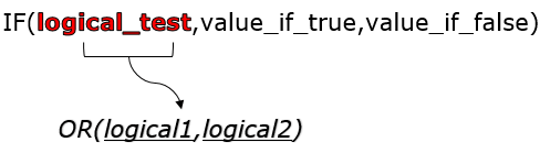
The IF function allows you to make a logical comparison between a value and what you expect by testing for a condition and returning a result if that condition is True or False.
-
=IF(Something is True, then do something, otherwise do something else)
But what if you need to test multiple conditions, where let’s say all conditions need to be True or False (AND), or only one condition needs to be True or False (OR), or if you want to check if a condition does NOT meet your criteria? All 3 functions can be used on their own, but it’s much more common to see them paired with IF functions.
Use the IF function along with AND, OR and NOT to perform multiple evaluations if conditions are True or False.
Syntax
-
IF(AND()) — IF(AND(logical1, [logical2], …), value_if_true, [value_if_false]))
-
IF(OR()) — IF(OR(logical1, [logical2], …), value_if_true, [value_if_false]))
-
IF(NOT()) — IF(NOT(logical1), value_if_true, [value_if_false]))
|
Argument name |
Description |
|
|
logical_test (required) |
The condition you want to test. |
|
|
value_if_true (required) |
The value that you want returned if the result of logical_test is TRUE. |
|
|
value_if_false (optional) |
The value that you want returned if the result of logical_test is FALSE. |
|
Here are overviews of how to structure AND, OR and NOT functions individually. When you combine each one of them with an IF statement, they read like this:
-
AND – =IF(AND(Something is True, Something else is True), Value if True, Value if False)
-
OR – =IF(OR(Something is True, Something else is True), Value if True, Value if False)
-
NOT – =IF(NOT(Something is True), Value if True, Value if False)
Examples
Following are examples of some common nested IF(AND()), IF(OR()) and IF(NOT()) statements. The AND and OR functions can support up to 255 individual conditions, but it’s not good practice to use more than a few because complex, nested formulas can get very difficult to build, test and maintain. The NOT function only takes one condition.

Here are the formulas spelled out according to their logic:
|
Formula |
Description |
|---|---|
|
=IF(AND(A2>0,B2<100),TRUE, FALSE) |
IF A2 (25) is greater than 0, AND B2 (75) is less than 100, then return TRUE, otherwise return FALSE. In this case both conditions are true, so TRUE is returned. |
|
=IF(AND(A3=»Red»,B3=»Green»),TRUE,FALSE) |
If A3 (“Blue”) = “Red”, AND B3 (“Green”) equals “Green” then return TRUE, otherwise return FALSE. In this case only the first condition is true, so FALSE is returned. |
|
=IF(OR(A4>0,B4<50),TRUE, FALSE) |
IF A4 (25) is greater than 0, OR B4 (75) is less than 50, then return TRUE, otherwise return FALSE. In this case, only the first condition is TRUE, but since OR only requires one argument to be true the formula returns TRUE. |
|
=IF(OR(A5=»Red»,B5=»Green»),TRUE,FALSE) |
IF A5 (“Blue”) equals “Red”, OR B5 (“Green”) equals “Green” then return TRUE, otherwise return FALSE. In this case, the second argument is True, so the formula returns TRUE. |
|
=IF(NOT(A6>50),TRUE,FALSE) |
IF A6 (25) is NOT greater than 50, then return TRUE, otherwise return FALSE. In this case 25 is not greater than 50, so the formula returns TRUE. |
|
=IF(NOT(A7=»Red»),TRUE,FALSE) |
IF A7 (“Blue”) is NOT equal to “Red”, then return TRUE, otherwise return FALSE. |
Note that all of the examples have a closing parenthesis after their respective conditions are entered. The remaining True/False arguments are then left as part of the outer IF statement. You can also substitute Text or Numeric values for the TRUE/FALSE values to be returned in the examples.
Here are some examples of using AND, OR and NOT to evaluate dates.

Here are the formulas spelled out according to their logic:
|
Formula |
Description |
|---|---|
|
=IF(A2>B2,TRUE,FALSE) |
IF A2 is greater than B2, return TRUE, otherwise return FALSE. 03/12/14 is greater than 01/01/14, so the formula returns TRUE. |
|
=IF(AND(A3>B2,A3<C2),TRUE,FALSE) |
IF A3 is greater than B2 AND A3 is less than C2, return TRUE, otherwise return FALSE. In this case both arguments are true, so the formula returns TRUE. |
|
=IF(OR(A4>B2,A4<B2+60),TRUE,FALSE) |
IF A4 is greater than B2 OR A4 is less than B2 + 60, return TRUE, otherwise return FALSE. In this case the first argument is true, but the second is false. Since OR only needs one of the arguments to be true, the formula returns TRUE. If you use the Evaluate Formula Wizard from the Formula tab you’ll see how Excel evaluates the formula. |
|
=IF(NOT(A5>B2),TRUE,FALSE) |
IF A5 is not greater than B2, then return TRUE, otherwise return FALSE. In this case, A5 is greater than B2, so the formula returns FALSE. |

Using AND, OR and NOT with Conditional Formatting
You can also use AND, OR and NOT to set Conditional Formatting criteria with the formula option. When you do this you can omit the IF function and use AND, OR and NOT on their own.
From the Home tab, click Conditional Formatting > New Rule. Next, select the “Use a formula to determine which cells to format” option, enter your formula and apply the format of your choice.

Using the earlier Dates example, here is what the formulas would be.

|
Formula |
Description |
|---|---|
|
=A2>B2 |
If A2 is greater than B2, format the cell, otherwise do nothing. |
|
=AND(A3>B2,A3<C2) |
If A3 is greater than B2 AND A3 is less than C2, format the cell, otherwise do nothing. |
|
=OR(A4>B2,A4<B2+60) |
If A4 is greater than B2 OR A4 is less than B2 plus 60 (days), then format the cell, otherwise do nothing. |
|
=NOT(A5>B2) |
If A5 is NOT greater than B2, format the cell, otherwise do nothing. In this case A5 is greater than B2, so the result will return FALSE. If you were to change the formula to =NOT(B2>A5) it would return TRUE and the cell would be formatted. |
Note: A common error is to enter your formula into Conditional Formatting without the equals sign (=). If you do this you’ll see that the Conditional Formatting dialog will add the equals sign and quotes to the formula — =»OR(A4>B2,A4<B2+60)», so you’ll need to remove the quotes before the formula will respond properly.
Need more help?

See also
You can always ask an expert in the Excel Tech Community or get support in the Answers community.
Learn how to use nested functions in a formula
IF function
AND function
OR function
NOT function
Overview of formulas in Excel
How to avoid broken formulas
Detect errors in formulas
Keyboard shortcuts in Excel
Logical functions (reference)
Excel functions (alphabetical)
Excel functions (by category)
Home / Excel Formulas / How to Combine IF and OR Functions in Excel
IF Function is one of the most powerful functions in excel. And, the best part is, that you can combine other functions with IF to increase its power.
Combining IF and OR functions is one of the most useful formula combinations in excel. In this post, I’ll show you why we need to combine IF and OR functions. And, why it’s highly useful for you.
Quick Intro
I am sure you have used both of these functions but let me give you a quick intro.
- IF – Use this function to test a condition. It will return a specific value if that condition is true, or else some other specific value if that condition is false.
- OR – Test multiple conditions. It will return true if any of those conditions is true, and false if all of those conditions are false.
The crux of both of the functions is IF function can test only one condition at a time. And, OR function can test multiple conditions but only return true/false. And, if we combine these two functions we can test multiple conditions with OR & return a specific value with IF.
How do IF and OR functions Work?
In the syntax of the IF function, have a logical test argument that we use to specify a condition to test.
IF(logical_test,value_if_true,value_if_false)
And, then it returns a value based on the result of that condition. Now, if we use OR function for that argument and specify multiple conditions for it.
If any of the conditions is true OR will return true and IF will return the specific value. And, if none of the conditions is true OR with return FALSE IF will return another specific value. In this way, we can test more than one value with the IF function. Let’s get into some real-life examples.
Examples
Here I have a table with stock details of two warehouses. Now the thing is I want to update the status in the table.
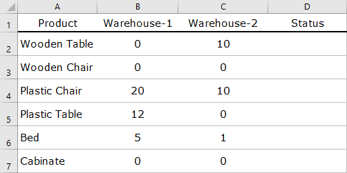
If there is no stock in both of the warehouses status should be “Out of Stock”. And, if there is stock in any of the warehouse status should be “In-Stocks”. So here I have to check two different conditions “Warehouse-1” & “Warehouse-2”.
And the formula will be.
=IF(OR(B2>0,C2>0),"In-Stock","Out of Stock")
In the above formula, if there is a value greater than zero in any of the cells (B2 & C2) OR function will return true, and IF will return the value “In-Stock”. But, if both cells have zero then OR will return false, and IF will return the value “Out of Stock”.
Download Sample File
- Ready
Last Words
Both of the functions are equally useful but when you combine them, you can use them in a better way. As I told you, by combining IF and Or functions you can test more than one condition. You can solve your two problems with this combination of functions.
And, if you want to Get Smarter than Your Colleagues check out these FREE COURSES to Learn Excel, Excel Skills, and Excel Tips and Tricks.
Содержание
- Use AND and OR to test a combination of conditions
- Use AND and OR with IF
- Sample data
- Using IF with AND, OR and NOT functions
- Examples
- Using AND, OR and NOT with Conditional Formatting
- Need more help?
- See also
- Formula examples using the functions OR AND IF in Excel
- Examples of using formulas with IF, AND, OR functions in Excel
- Formula with logical functions AND IF OR in excel
- Nesting the AND, OR, and IF Functions in Excel
- Build the Excel IF Statement
- Change the Formula’s Output
- Use the IF Statement in Excel
Use AND and OR to test a combination of conditions
When you need to find data that meets more than one condition, such as units sold between April and January, or units sold by Nancy, you can use the AND and OR functions together. Here’s an example:
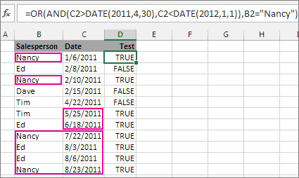
This formula nests the AND function inside the OR function to search for units sold between April 1, 2011 and January 1, 2012, or any units sold by Nancy. You can see it returns True for units sold by Nancy, and also for units sold by Tim and Ed during the dates specified in the formula.
Here’s the formula in a form you can copy and paste. If you want to play with it in a sample workbook, see the end of this article.
Use AND and OR with IF
You can also use AND and OR with the IF function.
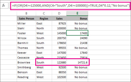
In this example, people don’t earn bonuses until they sell at least $125,000 worth of goods, unless they work in the southern region where the market is smaller. In that case, they qualify for a bonus after $100,000 in sales.
Let’s look a bit deeper. The IF function requires three pieces of data (arguments) to run properly. The first is a logical test, the second is the value you want to see if the test returns True, and the third is the value you want to see if the test returns False. In this example, the OR function and everything nested in it provides the logical test. You can read it as: Look for values greater than or equal to 125,000, unless the value in column C is «South», then look for a value greater than 100,000, and every time both conditions are true, multiply the value by 0.12, the commission amount. Otherwise, display the words «No bonus.»
Sample data
If you want to work with the examples in this article, copy the following table into cell A1 in your own spreadsheet. Be sure to select the whole table, including the heading row.
Источник
Using IF with AND, OR and NOT functions
The IF function allows you to make a logical comparison between a value and what you expect by testing for a condition and returning a result if that condition is True or False.
=IF(Something is True, then do something, otherwise do something else)
But what if you need to test multiple conditions, where let’s say all conditions need to be True or False ( AND), or only one condition needs to be True or False ( OR), or if you want to check if a condition does NOT meet your criteria? All 3 functions can be used on their own, but it’s much more common to see them paired with IF functions.
Use the IF function along with AND, OR and NOT to perform multiple evaluations if conditions are True or False.
IF(AND()) — IF(AND(logical1, [logical2], . ), value_if_true, [value_if_false]))
IF(OR()) — IF(OR(logical1, [logical2], . ), value_if_true, [value_if_false]))
IF(NOT()) — IF(NOT(logical1), value_if_true, [value_if_false]))
The condition you want to test.
The value that you want returned if the result of logical_test is TRUE.
The value that you want returned if the result of logical_test is FALSE.
Here are overviews of how to structure AND, OR and NOT functions individually. When you combine each one of them with an IF statement, they read like this:
AND – =IF(AND(Something is True, Something else is True), Value if True, Value if False)
OR – =IF(OR(Something is True, Something else is True), Value if True, Value if False)
NOT – =IF(NOT(Something is True), Value if True, Value if False)
Examples
Following are examples of some common nested IF(AND()), IF(OR()) and IF(NOT()) statements. The AND and OR functions can support up to 255 individual conditions, but it’s not good practice to use more than a few because complex, nested formulas can get very difficult to build, test and maintain. The NOT function only takes one condition.
Here are the formulas spelled out according to their logic:
=IF(AND(A2>0,B2 0,B4 50),TRUE,FALSE)
IF A6 (25) is NOT greater than 50, then return TRUE, otherwise return FALSE. In this case 25 is not greater than 50, so the formula returns TRUE.
IF A7 (“Blue”) is NOT equal to “Red”, then return TRUE, otherwise return FALSE.
Note that all of the examples have a closing parenthesis after their respective conditions are entered. The remaining True/False arguments are then left as part of the outer IF statement. You can also substitute Text or Numeric values for the TRUE/FALSE values to be returned in the examples.
Here are some examples of using AND, OR and NOT to evaluate dates.
Here are the formulas spelled out according to their logic:
IF A2 is greater than B2, return TRUE, otherwise return FALSE. 03/12/14 is greater than 01/01/14, so the formula returns TRUE.
=IF(AND(A3>B2,A3 B2,A4 B2),TRUE,FALSE)
IF A5 is not greater than B2, then return TRUE, otherwise return FALSE. In this case, A5 is greater than B2, so the formula returns FALSE.
Using AND, OR and NOT with Conditional Formatting
You can also use AND, OR and NOT to set Conditional Formatting criteria with the formula option. When you do this you can omit the IF function and use AND, OR and NOT on their own.
From the Home tab, click Conditional Formatting > New Rule. Next, select the “ Use a formula to determine which cells to format” option, enter your formula and apply the format of your choice.
Edit Rule dialog showing the Formula method» loading=»lazy»>
Using the earlier Dates example, here is what the formulas would be.
If A2 is greater than B2, format the cell, otherwise do nothing.
=AND(A3>B2,A3 B2,A4 B2)
If A5 is NOT greater than B2, format the cell, otherwise do nothing. In this case A5 is greater than B2, so the result will return FALSE. If you were to change the formula to =NOT(B2>A5) it would return TRUE and the cell would be formatted.
Note: A common error is to enter your formula into Conditional Formatting without the equals sign (=). If you do this you’ll see that the Conditional Formatting dialog will add the equals sign and quotes to the formula — =»OR(A4>B2,A4
Need more help?
See also
You can always ask an expert in the Excel Tech Community or get support in the Answers community.
Источник
Formula examples using the functions OR AND IF in Excel
Logical functions are designed to test one or several conditions, and perform the actions prescribed for each of the two possible results. Such results can only be logical TRUE or FALSE.
Excel contains several logical functions such as IF, IFERROR, SUMIF, AND, OR, and others. The last two are not used in practice, as a rule, because the result of their calculations may be one of only two possible options (TRUE, FALSE). When combined with the IF function, they are able to significantly expand its functionality.
Examples of using formulas with IF, AND, OR functions in Excel
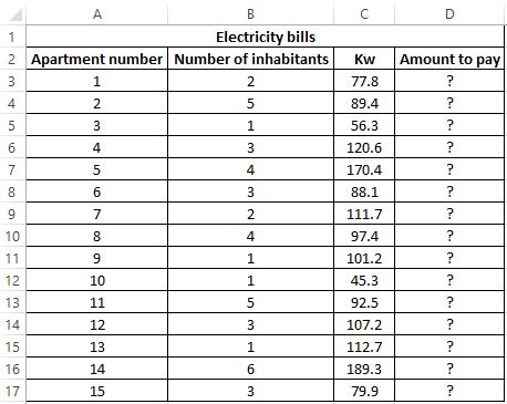
Example 1. When calculating the cost of the amount of consumed kW of electricity for subscribers, the following conditions are taken into account:
- If less than 3 people live in the apartment or less than 100 kW of electricity was consumed per month, the rate per 1 kW is 4.35$.
- In other cases, the rate for 1 kW is 5.25$.
Calculate the amount payable per month for several subscribers.
View source data table:
Perform the calculation according to the formula:
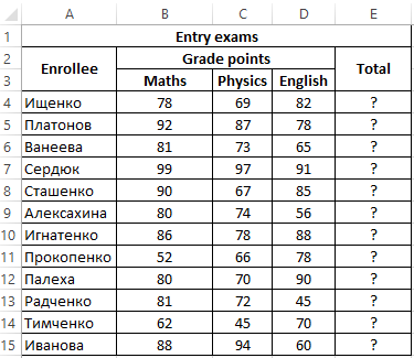
- OR (B3 Example 2. Applicants entering the university for the specialty «mechanical engineer» are required to pass 3 exams in mathematics, physics and English. The maximum score for each exam is 100. The average passing score for 3 exams is 75, while the minimum score in physics must be at least 70 points, and in mathematics it is 80. Determine applicants who have successfully passed the exams.
View source table:
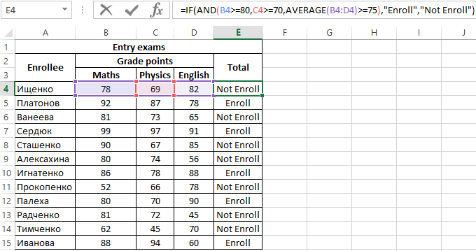
To determine the enrolled students use the formula:
- AND(B4>=80,C4>=70,AVERAGE(B4:D4)>=75) — checked logical expressions according to the condition of the problem;
- «Enroll» — the result, if the function AND returned the value TRUE (all expressions represented as its arguments, as a result of the calculations returned the value TRUE);
- «Not Enroll» — the result if AND returned FALSE.
Using the autocomplete function (double-click on the cursor marker in the lower right corner), we get the rest of the results:
Formula with logical functions AND IF OR in excel
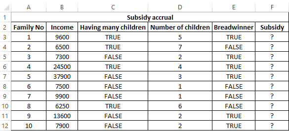
Example 3. Subsidies in the amount of 30% are charged to families with an average income below 8,000$, which are large or there is no main breadwinner. If the number of children is over 5, the amount of the subsidy is 50%. Determine who should receive subsidies and who should not.
View source table:
To check the criteria according to the condition of the problem, we write the formula:
- AND(B3 =IF( Logical_test ,[ Value_if_True ],[ Value_if_False])
As you can see, by default, you can check only one condition, for example, is e3 more than 20? Using the IF function, this check can be done as follows:
As a result, the text string “more” will be returned. If we need to find out if any value belongs to the specified interval, we will need to compare this value with the upper and lower limits of the intervals, respectively. For example, is the result of calculating e3 in the range from 20 to 25? When using the IF function alone, you must enter the following entry:
=IF(EXP(3)>20,IF(EXP(3) 20,EXP(3) 20,EXP(3) 0,EXP(3) ” means inequality, that is, more or less than some value. In this case, both expressions return the value TRUE, and the result of the execution of the IF function is the text string «true.» However, if an OR test was performed (MOD(EXP (3),1)<>0,EXP(3) 0 returns TRUE.
In practice, often used bundles IF + AND, IF + OR, or all three functions at once. Consider examples of similar use of these functions.
Источник
Nesting the AND, OR, and IF Functions in Excel
Using logical functions to test multiple conditions
Nesting functions in Excel refers to placing one function inside another. The nested function acts as one of the main function’s arguments. The AND, OR, and IF functions are some of Excel’s better known logical functions that are commonly used together.
Instructions in this article apply to Excel 2019, 2016, 2013, 2010, 2007; Excel for Microsoft 365, Excel Online, and Excel for Mac.
Build the Excel IF Statement
When using the IF, AND, and OR functions, one or all of the conditions must be true for the function to return a TRUE response. If not, the function returns FALSE as a value.
For the OR function (see row 2 in the image below), if one of these conditions is true, the function returns a value of TRUE. For the AND function (see row 3), all three conditions must be true for the function to returns a value of TRUE.
In the image below, rows 4 to 6 contain formulas where the AND and OR functions are nested inside the IF function.
:max_bytes(150000):strip_icc()/nesting-the-and-or-and-if-functions-r3-5c77de7cc9e77c0001e98ddc.jpg)
When the AND and OR functions are combined with the IF function, the resulting formula has much greater capabilities.
In this example, three conditions are tested by the formulas in rows 2 and 3:
- Is the value in cell A2 less than 50?
- Is the value in cell A3 not equal to 75?
- Is the value in cell A4 greater than or equal to 100?
Also, in all of the examples, the nested function acts as the IF function’s first argument. This first element is known as the Logical_test argument.
=IF(OR(A2 75,A4>=100),»Data Correct»,»Data Error»)
Change the Formula’s Output
In all formulas in rows 4 to 6, the AND and OR functions are identical to their counterparts in rows 2 and 3 in that they test the data in cells A2 to A4 to see if it meets the required condition.
The IF function is used to control the formula’s output based on what is entered for the function’s second and third arguments. Examples of this output can be text as seen in row 4, a number as seen in row 5, the output from the formula, or a blank cell.
In the case of the IF/AND formula in cell B5, since not all three cells in the range A2 to A4 are true — the value in cell A4 is not greater than or equal to 100 — the AND function returns a FALSE value. The IF function uses this value and returns its Value_if_false argument — the current date supplied by the TODAY function.
On the other hand, the IF/OR formula in row four returns the text statement Data Correct for one of two reasons:
The OR value has returned a TRUE value — the value in cell A3 does not equal 75.
The IF function then used this result to return its Value_if_false argument: Data Correct.
Use the IF Statement in Excel
The next steps cover how to enter the IF/OR formula located in cell B4 from the example. These same steps can be used to enter any of the IF formulas in these examples.
:max_bytes(150000):strip_icc()/nesting-the-and-or-and-if-functions-r4-5c77df49c9e77c00012f8178.jpg)
There are two ways to enter formulas in Excel. Either type the formula in the Formula Bar or use the Function Arguments dialog box. The dialog box takes care of the syntax such as placing comma separators between arguments and surrounding text entries in quotation marks.
The steps used to enter the IF/OR formula in cell B4 are as follows:
Select cell B4 to make it the active cell.
On the ribbon, go to Formulas.
Select Logical to open the function dropdown list.
Choose IF in the list to open the Function Arguments dialog box.
:max_bytes(150000):strip_icc()/nesting-the-and-or-and-if-functions-r5-5c77dfcdc9e77c00012f8179.jpg)
Place the cursor in the Logical_test text box.
Enter the complete OR function:
Place the cursor in the Value_if_true text box.
Type Data Correct.
Place the cursor in the Value_if_false text box.
Type Data Error.
:max_bytes(150000):strip_icc()/nesting-the-and-or-and-if-functions-r6-5c77e07746e0fb00011bf26b.jpg)
Select OK to complete the function.
The formula displays the Value_if_true argument of Data Correct.
Select cell B4 to see the complete function in the formula bar above the worksheet.
Источник
We use the IF statement in Excel to test one condition and return one value if the condition is met and another if the condition is not met.
However, we use multiple or nested IF statements when evaluating numerous conditions in a specific order to return different results.
This tutorial shows four examples of using nested IF statements in Excel and gives five alternatives to using multiple IF statements in Excel.
General Syntax of Nested IF Statements (Multiple IF Statements)
The general syntax for nested IF statements is as follows:
=IF(Condition1, Value_if_true1, IF(Condition2, Value_if_true2, IF(Condition3, Value_if_true3, Value_if_false)))
This formula tests the first condition; if true, it returns the first value.
If the first condition is false, the formula moves to the second condition and returns the second value if it’s true.
Each subsequent IF function is incorporated into the value_if_false argument of the previous IF function.
This process continues until all conditions have been evaluated, and the formula returns the final value if none of the conditions is true.
The maximum number of nested IF statements allowed in Excel is 64.
Now, look at the following four examples of how to use nested IF statements in Excel.
Example #1: Use Multiple IF Statements to Assign Letter Grades Based on Numeric Scores
Let’s consider the following dataset showing some students’ scores on a Math test.

We want to use nested IF statements to assign student letter grades based on their scores.
We use the following steps:
- Select cell C2 and type in the below formula:
=IF(B2>=90,"A",IF(B2>=80,"B",IF(B2>=70,"C",IF(B2>=60,"D","F"))))

- Click Enter in the cell to get the result of the formula in the cell.
- Copy the formula for the rest of the cells in the column
The assigned letter grades appear in column C.

Explanation of the formula
=IF(B2>=90,”A”,IF(B2>=80,”B”,IF(B2>=70,”C”,IF(B2>=60,”D”,”F”))))
This formula evaluates the value in cell B2 and assigns an “A” if the value is 90 or greater, a “B” if the value is between 80 and 89, a “C” if the value is between 70 and 79, a “D” if the value is between 60 and 69, and an “F” if the value is less than 60.
Notice that it can be challenging to keep track of which parentheses go with which arguments in nested IF functions.
Therefore, as we enter the formula, Excel uses different colors for the parentheses at each level of the nested IF functions to make it easier to see which parts of the formula belong together.

Also read: How to use Excel If Statement with Multiple Conditions Range
Example #2: Use Multiple IF Statements to Calculate Commission Based on Sales Volume
Here’s the dataset showing the sales of specific salespeople in a particular month.

We want to use multiple IF statements to calculate the tiered commission for the salespeople based on their sales volume.
We proceed as follows:
- Select cell C2 and enter the following formula:
=IF(B2>=40000, B2*0.14,IF(B2>=20000,B2*0.12,IF(B2>=10000,B2*0.105,IF(B2>0,B2*0.08,0))))

- Press the Enter key to get the result of the formula.
- Double-click or drag the Fill Handle to copy the formula down the column.
The commission for each salesperson is displayed in column D.

Explanation of the formula
=IF(B2>=40000, B2*0.14,IF(B2>=20000,B2*0.12,IF(B2>=10000,B2*0.105,IF(B2>0,B2*0.08,0))))
This formula evaluates the value in cell B2 and then does the following:
- If the value in cell B2 is greater than or equal to 40,000, the figure is multiplied by 14% (0.14).
- If the figure in cell B2 is less than 40,000 but greater than or equal to 20,000, the value is multiplied by 12% (0.12).
- If the number in cell B2 is less than 20,000 but greater than or equal to 10,000, the figure is multiplied by 10.5% (0.105).
- If the value in cell B2 is less than 10,000 but greater than 0 (zero), the number is multiplied by 8% (0.08).
- If the value in cell B2 is 0 (zero), 0 (zero) is returned.
Example #3: Use Multiple IF Statements to Assign Sales Performance Rating Based On Sales Target Achievement
The following is a dataset showing regional sales data of a specific technology company in a particular year.

We want to use multiple IF statements to assign a sales performance rating to each region based on their sales target achievement.
We use the following steps:
- Select cell C2 and type in the below formula:
=IF(B2>500000, "Excellent", IF(B2>400000, "Good", IF(B2>275000, "Average", "Poor")))

- Click Enter on the Formula bar.
- Drag or double-click the Fill Handle to copy the formula down the column.
The performance ratings of the regions are shown in column C.

Explanation of the formula
=IF(B2>500000, “Excellent”, IF(B2>400000, “Good”, IF(B2>275000, “Average”, “Poor”)))
In this formula, if the sales target in cell B2 is greater than 500,000, the formula returns “Excellent.”
If it’s between 400,000 and 500,000, the formula returns “Good.”
If it’s between 275,000 and 400,000, the formula returns “Average.” And if it’s below 275,000, the formula returns “Poor.”
Example #4: Use Multiple IF Statements in Excel to Check For Errors and Return Error Messages
Suppose we have the following dataset of students’ English test scores. Some scores are less than 0 or greater than 100, and there are no scores in some cases.

We want to use nested IF statements to check for scores in column B and display error messages in column C if there are no scores or the scores are less than 0 or greater than 100.
If the score in column B is valid, we want the formula to return an empty string in column C.
Here are the steps to follow:
- Select cell C2 and enter the following formula:
=IF(OR(B2<0,B2>100),"Score out of range",IF(ISBLANK(B2),"Invalid score",""))

- Click Enter on the Formula bar.
- Drag the Fill Handle to copy the formula down the column.
The error messages are shown in column C.

Explanation of the formula
=IF(OR(B2<0,B2>100),”Score out of range”,IF(ISBLANK(B2),”Invalid score”,””))
This formula uses the OR function to check if the score in cell B2 is less than 0 or greater than 100, and if it is, it returns the error message “Score out of range.”
The formula also uses the ISBLANK function to check if cell B2 is blank, and if it is, it returns the error message “Invalid score.”
If there is no error, the formula returns an empty string, meaning no message is displayed in column B.
Alternatives to Using Multiple IF Statements in Excel
Formulas using nested IF statements can become difficult to read and manage if we have more than a few conditions to test.
In addition, if we exceed the maximum allowed limit of 64 nested IF statements, we will get an error message.
Fortunately, Excel offers alternative ways to use instead of nested IF functions, especially when we need to test more than a few conditions.
We present the alternative ways in this tutorial.
Alternative #1: Use the IFS Function
The IFS function tests whether one or more conditions are met and returns a value corresponding to the first TRUE condition.
Before the release of the IFS function in 2018 as part of the Excel 365 update, the only way to test multiple conditions and return a corresponding value in Excel was to use nested IF statements.
However, multiple IF statements have the downside of resulting in unwieldy formulas that are difficult to read and maintain.
In some situations, the IFS function is designed to replace the need for multiple IF functions.
The syntax of the IFS function is more straightforward and easier to read than nested IF statements, and it can handle up to 127 conditions.
Here’s an example:
Let’s consider the following dataset showing some students’ scores on a Math test.

We want to use the IFS function to assign letter grades to the students based on their scores.
We use the following steps:
- Select cell C2 and type in the below formula:
=IFS(B2>=90, "A", B2>=80, "B", B2>=70, "C", B2>=60, "D", B2<60, "F")

- Click Enter on the Formula bar.
- Drag or double-click the Fill Handle to copy the formula down the column.
The student’s letter grades are shown in column C.

Explanation of the formula
=IFS(B2>=90, “A”, B2>=80, “B”, B2>=70, “C”, B2>=60, “D”, B2<60, “F”)
This formula tests the score in cell B2 against each condition and returns the corresponding grade letter when the condition is true.
Limitation of IFS Function
The IFS function in Excel is designed to simplify complex nested IF statements.
However, there are situations where the IFS function may not be able to replace nested IF functions completely.
One such situation is when you must calculate or operate based on a condition or set of conditions.
While the IFS function can return a value or text string based on a condition, it cannot perform calculations or operations on that value like nested IF statements.
Another situation where the IFS function may be less useful is when you need to test for a range of conditions rather than just a specific set.
This is because the IFS function requires you to specify each condition and corresponding result separately, which can become cumbersome if you have many conditions to test—in contrast, nested IF statements allow you to test for a range of conditions using logical operators like AND and OR.
The IFS function is a powerful tool for simplifying complex logical tests in Excel.
However, there may be situations where nested IF statements are more appropriate for your needs.
We recommend that you consider both options and choose the one that best fits the specific requirements of your task.
Alternative #2: Use Nested IF Functions
We can use multiple IFS functions in a formula if we have more than one condition to test.
For example, let’s say we have the following dataset of student names and scores on a Physics test in columns A and B.

We want to assign a letter grade to each score and include a pass or fail designation based on whether the score is above or below 75.
Here are the steps to use:
- Select cell C2 and enter the following formula
=IFS(B2>=90,"A",B2>=80,"B",B2>=70,"C",B2>=60,"D",B2<60,"F")&" "&IFS(B2>=75,"Pass",B2<75,"Fail")

- Click Enter on the Formula bar.
- Drag or double-click the Fill Handle to copy the formula down the column.
The letter grade and designation of the student scores are displayed in column C.

Explanation of the formula
=IFS(B2>=90,”A”,B2>=80,”B”,B2>=70,”C”,B2>=60,”D”,B2<60,”F”)&” “&IFS(B2>=75,”Pass”,B2<75,”Fail”)
This formula uses the first IFS function to assign a letter grade based on the score in column A and the second IFS function to give a pass/fail designation based on the score in column A.
The two IFS functions are combined using the ampersand (&) operator to create a single text string that displays each score’s letter grade and pass/fail designation.
Alternative #3: Use the Combination of CHOOSE and XMATCH Functions
The CHOOSE function selects a value or action from a value list based on an index number.
The XMATCH function locates and returns the relative position of an item in an array. We can combine these functions in a formula instead of nested IF functions.
Here’s an example:
Suppose we have the following dataset showing some students’ scores and letter grades on a Biology test.

We want to use a formula combining the CHOOSE and XMATCH functions to assign corresponding grade points in column D to each letter grade.
We use the following steps:
- Select cell D2 and type in the below formula:
=CHOOSE(XMATCH(C2,{"F","E","D","C","B","A"},0),0,1,2,3,4,5)

- Click Enter on the Formula bar.
- Drag or double-click the Fill Handle to copy the formula down the column.
The grade points for each student are displayed in column D.

Explanation of the formula
=CHOOSE(XMATCH(C2,{“F”,”E”,”D”,”C”,”B”,”A”},0),0,1,2,3,4,5)
This formula applies the XMATCH function to find the position of the letter grade in the array {“F”,”E”,”D”,”C”,”B”,”A”}, and then uses the CHOOSE function to return the corresponding grade points.
Alternative #4: Use the VLOOKUP Function
The VLOOKUP function looks for a value in the leftmost column of a table and then returns a value in the same row from a specified column.
We can use the VLOOKUP function instead of nested IF functions in Excel.
The following is an example of using the VLOOKUP function instead of nested IF functions in Excel:
Suppose we have the following dataset showing some students’ scores and letter grades on a Biology test.

We want to use the VLOOKUP function to assign grade points to each student’s letter grade in column D.
We use the steps below:
- Create a table that lists the grades and their corresponding grade points in cell range F1:G7.

- In cell D2, type the following formula:
=VLOOKUP(C2,$F$2:$G$7,2,FALSE)
Note: Use the dollar signs to lock down the cell range F2:G7.

- Click Enter on the Formula bar.
- Drag or double-click the Fill Handle to copy the formula down the column.
The grade points for each student appear in column D.

Explanation of the formula
=VLOOKUP(C2,$F$2:$G$7,2,FALSE)
This formula uses the VLOOKUP function to look up the grade in cell C2 in the table in F2:G7 and return the corresponding grade point in the second column (i.e., column G).
The “FALSE” argument ensures that an exact match is required.
Alternative #5: Use a User-Defined Function
If you need to test more than a few conditions, consider creating a User Defined Function in VBA that can handle many conditions.
Here’s an example of using VBA code to replace nested IF functions in Excel:
Suppose we have the following dataset showing the sales of specific salespeople in a particular month.

We want to use a User Defined Function to calculate the commission for each salesperson based on the following rates:
- If the total sales are less than $10,000, the commission rate is 8%.
- If the total sales are equal to or greater than $10,000 but less than $20,000, the commission rate is 10.5%.
- If the total sales are equal to or greater than $20,000 but less than $40,000, the commission rate is 12%.
- If the sales are equal to or greater than $40,000, the commission rate is 14%
We use the following steps:
- Open the worksheet containing the sales dataset.
- Press Alt + F11 to launch the Visual Basic Editor.
- Click Insert on the menu bar and choose Module to insert a new module.

- Enter the following VBA code.
'Code developed by Steve Scott from https://spreadsheetplanet.com
Function COMMISSION(Sales As Double) As Double
    Const Rate1 = 0.08
    Const Rate2 = 0.105
    Const Rate3 = 0.12
    Const Rate4 = 0.14

'Calculate sales commissions

    Select Case Sales
        Case 0 To 9999.99: COMMISSION = Sales * Rate1
        Case 10000 To 19999.99: COMMISSION = Sales * Rate2
        Case 20000 To 39999.99: COMMISSION = Sales * Rate3
        Case Is >= 40000: COMMISSION = Sales * Rate4
    End Select

End Function
- Save the function procedure and the workbook as a Macro-Enabled Workbook.
- Press Alt + F11 to switch to the active worksheet with the sales dataset.
- Select cell C2 and enter the following formula:
=COMMISSION(B2)

- Click Enter on the Formula bar.
- Drag or double-click the Fill Handle to copy the formula down the column.
The commission for each salesperson is displayed in column C.

This VBA function takes the sales amount as an argument and returns the corresponding commission.
The User-Defined Function is a much simpler and easier-to-read solution than using nested IF functions.
This tutorial showed four examples of using nested IF statements in Excel and gave five alternatives to using multiple IF statements in Excel. We hope you found the tutorial helpful.
Other Excel tutorials you may find useful:
- Excel Logical Test Using Multiple If Statements in Excel [AND/OR]
- How to Compare Two Columns in Excel (using VLOOKUP & IF)
- Using IF Function with Dates in Excel (Easy Examples)
- COUNTIF Greater Than Zero in Excel
- BETWEEN Formula in Excel (Using IF Function) – Examples
- Count Cells Less than a Value in Excel (COUNTIF Less)
When you combine each one of them with an IF statement, they read like this:
- AND – =IF(AND(Something is True, Something else is True), Value if True, Value if False)
- OR – =IF(OR(Something is True, Something else is True), Value if True, Value if False)
- NOT – =IF(NOT(Something is True), Value if True, Value if False)
How do I apply conditional formatting to an entire column?
Five steps to apply conditional formatting across an entire row
- Highlight the data range you want to format.
- Choose Format > Conditional formatting… in the top menu.
- Choose “Custom formula is” rule.
- Enter your formula, using the $ sign to lock your column reference.
How do you add a rule in conditional formatting?
Create a custom conditional formatting rule
- Select the range of cells, the table, or the whole sheet that you want to apply conditional formatting to.
- On the Home tab, click Conditional Formatting.
- Click New Rule.
- Select a style, for example, 3-Color Scale, select the conditions that you want, and then click OK.
What are the four types of conditional formatting?
Conditional Formatting Examples : Types
- Background Color Shading (of cells)
- Foreground Color Shading (of fonts)
- Data Bars.
- Icons (which have 4 different image types)
- Values.
What is condition formatting?
Conditional formatting is a feature of Excel which allows you to apply a format to a cell or a range of cells based on certain criteria. For example the following rules are used to highlight cells in the conditional_format.py example: worksheet.
How do you conditional format a cell based on value?
Excel formulas for conditional formatting based on cell value
- Select the cells you want to format.
- On the Home tab, in the Styles group, click Conditional formatting > New Rule…
- In the New Formatting Rule window, select Use a formula to determine which cells to format.
- Enter the formula in the corresponding box.
How do I automatically change the cell color in Excel based on text?
Apply conditional formatting based on text in a cell
- Select the cells you want to apply conditional formatting to. Click the first cell in the range, and then drag to the last cell.
- Click HOME > Conditional Formatting > Highlight Cells Rules > Text that Contains.
- Select the color format for the text, and click OK.
How can I tell the color of a cell in Excel?
Select the cell that is formatted with the color you want to check. Display the Home tab of the ribbon. Click the down-arrow at the right side of the Fill Color tool, in the Font group. Excel displays a small palette of colors and some other options.
How do I change the color of a cell in Excel with a formula?
You can color-code your formulas using Excel’s conditional formatting tool as follows. Select a single cell (such as cell A1). From the Home tab, select Conditional Formatting, New Rule, and in the resulting New Formatting Rule dialog box, select Use a formula to determine which cells to format.
Can I sum by color in Excel?
Select a range or ranges where you want to count colored cells or/and sum by color if you have numerical data. Press and hold Ctrl, select one cell with the needed color, and then release the Ctrl key. Press Alt+F8 to open the list of macros in your workbook. Sum is the sum of values of all red cells in the Qty.
Nesting functions in Excel refers to placing one function inside another. The nested function acts as one of the main function’s arguments. The AND, OR, and IF functions are some of Excel’s better known logical functions that are commonly used together.
Instructions in this article apply to Excel 2019, 2016, 2013, 2010, 2007; Excel for Microsoft 365, Excel Online, and Excel for Mac.
Build the Excel IF Statement
When using the IF, AND, and OR functions, one or all of the conditions must be true for the function to return a TRUE response. If not, the function returns FALSE as a value.
For the OR function (see row 2 in the image below), if one of these conditions is true, the function returns a value of TRUE. For the AND function (see row 3), all three conditions must be true for the function to returns a value of TRUE.
In the image below, rows 4 to 6 contain formulas where the AND and OR functions are nested inside the IF function.
When the AND and OR functions are combined with the IF function, the resulting formula has much greater capabilities.
In this example, three conditions are tested by the formulas in rows 2 and 3:
- Is the value in cell A2 less than 50?
- Is the value in cell A3 not equal to 75?
- Is the value in cell A4 greater than or equal to 100?
Also, in all of the examples, the nested function acts as the IF function’s first argument. This first element is known as the Logical_test argument.
=IF(OR(A2<50,A3<>75,A4>=100),"Data Correct","Data Error")
=IF(AND(A2<50,A3<>75,A4>=100),1000,TODAY())
Change the Formula’s Output
In all formulas in rows 4 to 6, the AND and OR functions are identical to their counterparts in rows 2 and 3 in that they test the data in cells A2 to A4 to see if it meets the required condition.
The IF function is used to control the formula’s output based on what is entered for the function’s second and third arguments. Examples of this output can be text as seen in row 4, a number as seen in row 5, the output from the formula, or a blank cell.
In the case of the IF/AND formula in cell B5, since not all three cells in the range A2 to A4 are true — the value in cell A4 is not greater than or equal to 100 — the AND function returns a FALSE value. The IF function uses this value and returns its Value_if_false argument — the current date supplied by the TODAY function.
On the other hand, the IF/OR formula in row four returns the text statement Data Correct for one of two reasons:
-
The OR value has returned a TRUE value — the value in cell A3 does not equal 75.
-
The IF function then used this result to return its Value_if_false argument: Data Correct.
Use the IF Statement in Excel
The next steps cover how to enter the IF/OR formula located in cell B4 from the example. These same steps can be used to enter any of the IF formulas in these examples.
There are two ways to enter formulas in Excel. Either type the formula in the Formula Bar or use the Function Arguments dialog box. The dialog box takes care of the syntax such as placing comma separators between arguments and surrounding text entries in quotation marks.
The steps used to enter the IF/OR formula in cell B4 are as follows:
-
Select cell B4 to make it the active cell.
-
On the ribbon, go to Formulas.
-
Select Logical to open the function dropdown list.
-
Choose IF in the list to open the Function Arguments dialog box.
-
Place the cursor in the Logical_test text box.
-
Enter the complete OR function:
OR(A2<50,A3<>75,A4>=100)
-
Place the cursor in the Value_if_true text box.
-
Type Data Correct.
-
Place the cursor in the Value_if_false text box.
-
Type Data Error.
-
Select OK to complete the function.
-
The formula displays the Value_if_true argument of Data Correct.
-
Select cell B4 to see the complete function in the formula bar above the worksheet.
Thanks for letting us know!
Get the Latest Tech News Delivered Every Day
Subscribe
To write an IF, AND, OR array formula in Excel 365, we must use the arithmetic operators * (multiplication) and + (addition). Why it’s so?
If we take the logical AND, OR with the IF in Excel 365 to spill the result, we won’t get our expected result.
I mean, such a formula won’t support a range/array in evaluation. Even if it supports, it won’t return an array result.
So we will replace the AND logical operator with the * (multiplication) and OR with the + (addition) arithmetic operators.
Coding the formula with the said two operators is very simple and easily readable.
I think I can convince you the same with the examples below.
Example to IF, AND, OR in Excel 365 (Non-Array Formula)
Imagine a user played a game three times, and we have recorded his scores out of 100 in cells A2, B2, and C2.
We want to perform the following three logical tests on the scores individually.
- If all scores are >=80, return OK.
- If any of the two scores are >=80, return OK.
- Finally, if any of the scores is >=80, return OK.
Logical Tests Using IF, AND, OR Functions
In Excel, we can perform the above three logical tests as follows.
1. E2 (If all scores are >=80, return OK)
=IF(AND(A2>=80,B2>=80,C2>=80),"OK","NOT OK")I have used the AND function with IF in the above Excel formula to test if all the three logical tests return TRUE.
2. F2 (If any of the two scores are >=80, return OK)
We must use the following logic (two parts) to test if any two logical tests return TRUE.
AND Part:-
a) Value 1>=80 and value 2>=80.
b) Value 1>=80 and value 3>=80.
c) Value 2>=80 and value 3>=80.
OR Part:-
a) The OR evaluates to TRUE if any two of the above three AND tests return TRUE.
So the formula will be as follows.
=IF(OR(AND(A2>=80,B2>=80),AND(A2>=80,C2>=80),AND(B2>=80,C2>=80)),"OK","NOT OK")It is an example of the IF, AND, OR logical test in Excel.
3. G2 (if any of the scores is >=80, return OK)
=IF(OR(A2>=80,B2>=80,C2>=80),"OK","NOT OK")Here I have used the OR function with IF to test if any of the three logical tests return TRUE.
As I have already mentioned, we can’t write an IF, AND, OR array formula as above in Excel 365.
Logical Tests Using IF, *, + Formula
Let’s substitute the above three formulas by replacing AND, OR with multiplication and addition.
But that’s not enough. Then?
The below formulas are self-explanatory.
1. E2 Formula
=IF((A2:A8>=80)*(B2:B8>=80)*(C2:C8>=80),"OK","NOT OK")How the multiplication replaces the logical function OR above?
Each test in the formula returns either TRUE or FALSE. If all the criteria are met, it will be =IF((TRUE*TRUE*TRUE),"OK","NOT OK").
We can even replace the multiplication operator here with addition.
=IF((A2:A8>=80)+(B2:B8>=80)+(C2:C8>=80)>2,"OK","NOT OK")Please remember that the value of TRUE is 1, and FALSE is 0.
2. F2 Formula
=IF((A2:A8>=80)+(B2:B8>=80)+(C2:C8>=80)>1,"OK","NOT OK")3. G2 Formula
=IF((A2:A8>=80)+(B2:B8>=80)+(C2:C8>=80)>0,"OK","NOT OK")Above I have tried to simplify the use of the logical operators within the IF function.
Now let’s open an Excel Spreadsheet and enter the scores of multiple players in the range A2:C8 as below.

So the values to evaluate are in cell range A2:C8.
I have inserted the following three IF, AND, OR array formulas in cells E2, F2, and G2, respectively.
1. E2 Array Formula
=IF((A2:A8>=80)*(B2:B8>=80)*(C2:C8>=80),"OK","NOT OK")2. F2 Array Formula
=IF((A2:A8>=80)+(B2:B8>=80)+(C2:C8>=80)>1,"OK","NOT OK")3. G2 Array Formula
=IF((A2:A8>=80)+(B2:B8>=80)+(C2:C8>=80)>0,"OK","NOT OK")If any of the above formulas return #SPILL!, please empty the cells down in that column.
Nested IF, AND, OR Combination in Excel 365
I want to assign grades based on the scores above.
In that case, we may require to write a nested IF, AND, OR combination array formula in Excel 365.
Here is how.
In the above example, we have used three formulas for the below three logical tests.
- If all scores are >=80, return OK.
- If any of the two scores are >=80, return OK.
- Finally, if any of the scores is >=80, return OK.
There each test returns OK or NOT OK.
Instead of that, here, I want the tests to return GR-1, GR-2, and GR-3.
- If all scores are >=80, return GR-1.
- If any of the two scores are >=80, return GR-2.
- Finally, if any of the scores is >=80, return GR-3.
For that, we should combine the above three IF, AND, OR Array Formulas.
How?
In the E2 formula, replace “OK” with “GR-1” and “NOT OK” with the F2 formula.
In that combined (E2 and F2) formula, replace “OK” with “GR-2” and “NOT OK” with the G2 formula.
Then, in the combined E2, F2, and G2 formula, replace “OK” with “GR-3” and replace “NOT OK” with “F.”
Here it is.

=IF(
     (A2:A8>=80)*(B2:B8>=80)*(C2:C8>=80),"GR-1",
     IF(
        (A2:A8>=80)+(B2:B8>=80)+(C2:C8>=80)>1,"GR-2",
        IF(
           (A2:A8>=80)+(B2:B8>=80)+(C2:C8>=80)>0,"GR-3","F"
        )
     )
)
We can call it a nested IF, AND, OR combination array formula.
Related:- How to Use the IFS Function in Excel 365.
Excel AND + OR Functions: Full Guide (with IF Formulas)
The AND and OR functions returns True or False if certain conditions are met.
Combined with other functions, like IF, that enables multiple criteria logic in your formulas.
In this guide, I’ll walk you through all of this, step-by-step 👍🏼
If you want to tag along, download the sample workbook here.
We use the data in the following table to learn how to apply OR and AND function with the IF function in excel.

The OR function
The OR function is one of the most important logical functions in excel 😯
The OR function in Excel returns True if at least one of the criteria evaluates to true.
If all the arguments evaluate as False, then the OR function returns False.
The syntax of the OR function in Excel is OR(logical1, [logical2], …).
Assume that employees are eligible for an incentive if they achieve a value or volume target of 75% or more 🏆
Let’s try OR function for the above example.
- Enter an equal sign and select the OR function.
You will see below in the formula bar.
=OR(

- Supply the first logical value to evaluate as the first argument.
You can write logical values to test using logical operators.
In this case, we want to first test, whether the value target achievement is greater than or equal to 75%.
So, we can give the cell reference and write the condition >=75%.
Now the formula is,
=OR(B3>=75%

- Enter a comma and enter the 2nd logical value for the logical test.
Then, we enter the logical value for the volume target.
Now, the updated formula is;
=OR(B3>7=75%,C3>=75%

- Close the parentheses and press enter.
The below Excel formula evaluates arguments.
=OR(B3>7=75%,C3>=75%)
Then returns true if at least one of the value or volume target achievements is greater than or equal to 75%. If both value and volume target achievements are below 75%, the OR function returns False.

Pro Tip:
Now you have learned, the OR function returns True even when more than one condition evaluates to “True”.
Do you think you have to combine the OR function with the NOT function?
No. Excel has a simple solution 😜
You have to use the XOR function.
Apply the below XOR formula to the above example and see how the results are changing.
=XOR(B3>7=75%,C3>=75%)

You can see that Mary’s result is “False” as her achievements are not satisfying the one and only condition.
OR function IF formula example
Isn’t it boring to see only “True or false” values? 🥱
Don’t you like to get something other than True or False values? 👍
You just need to combine the OR function with the IF function in Excel.
Let’s say, we want the function to return “Eligible” if at least one of the value or volume target achievements is greater than or equal to 75%.
Also, return “Not eligible”, if both value and volume target achievements are less than 75%.
- Enter the equal sign and select the IF function.
Now, the formula bar will show;

- Enter the OR function that we have learned in the previous section.
The updated formula should be like this.
=IF(OR(B3>=75%,C3>=75%)

- Enter the specific value you want the function to return when the result of the logical test is True.
In this case, we want to get “Eligible”.
So, we enter the word eligible within quotes.
Now, the formula is;
=IF(OR(B3>=75%,C3>=75%),”Eligible”

If you want to enter text values for the arguments, you have to enter them within quotes. However, you don’t need to enter True or false values within quotes. Excel automatically evaluates arguments provided with true or false values.
- Enter the specific value you want the function to return when the result of the logical test is False.
In this case, we want to get “Not Eligible”.
Now, the updated formula is;
=IF(OR(B3>=75%,C3>=75%),”Eligible”,”Not Eligible”

- Close the parentheses and press “Enter”.

The AND function
AND function is another important logical function in excel.
This function returns true all of the multiple criteria are true.
Otherwise, the AND function returns False.
The syntax of the AND function in Excel is AND(logical1, [logical2], …).
Say that employees are entitled to an incentive if they achieve more than or equal to 75% for both the value target and volume target.
Let’s try AND function for the above example.
- Enter an equal sign and select the AND function.
You will see below in the formula bar.
=AND(

- Enter all logical values to test using logical operators.
So, you can enter the following formula.
=AND(B3>=75%,C3>=75%

- Close the parentheses and press “Enter”.

You can see that the AND function returns true only when both the value and volume target achievements exceed or are equal to 75% 🥳
However, there is limited usage of AND function if we do not combine it with other functions in Excel 🤔
Let’s see an example with a combination of the IF function and AND function.
AND function IF formula example
Let’s say, we want the function to return “Eligible”, only when both value and volume target achievements are more than or equal to 75%.
Otherwise, we want to get “Not eligible”
- Enter the equals sign and select the IF function.
Now, the formula bar will show;

- Enter the AND function that we have learned in the previous section.
The updated formula should be like this.
=IF(AND(B3>=75%,C3>=75%)

- Enter the specific value you want the function to return when the result of the logical test is True.
In this case, we want to get “Eligible”.
So, we enter the word eligible within quotes.
Now, the formula is;
=IF(AND(B3>=75%,C3>=75%),”Eligible”

- Enter the specific value you want the function to return when the result of the logical test is False.
In this case, we want to get “Not Eligible”.
Now, the updated formula is;
=IF(AND(B3>=75%,C3>=75%),”Eligible”,”Not Eligible”

- Close the parentheses and press “Enter”.

You can see that we get “Eligible” only when all of the multiple conditions are True. Otherwise, functions will return false 😍
Any empty cells in a logical function’s argument are ignored.

That’s it – Now what?
Well done 👏🏻
Now you know how to use the OR and AND functions in Excel.
Using the above examples, you have learned that OR and AND functions are more powerful when we combine them with other Excel functions 💪🏻
To learn more about other important functions such as IF, SUMIF, and VLOOKUP functions, all you need to do is enroll in my free 30-minute online Excel course.
Other resources
When you are using OR and AND functions, it is extremely important to use logical operators correctly ⚡
Read our article about logical operators, if you want to refresh your knowledge about them.
Also, Read our articles about the IF function, nested IF function, and SUMIF function and apply OR and AND functions more effectively 🥳
Frequently asked questions
You can enter 2 conditions or more for the logical test argument of the IF function using the following formulas.
If you want to satisfy,
- Both conditions – use the AND function.
- At least one condition – use the OR function
- Only one condition – use the XOR function.
Yes. We can use multiple logical functions with the IF function in Excel.
You can combine OR and AND functions to evaluate the arguments appropriately.
Kasper Langmann2023-02-23T11:04:48+00:00
Page load link