
Freeze panes to lock rows and columns
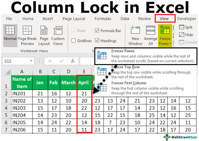
To keep an area of a worksheet visible while you scroll to another area of the worksheet, go to the View tab, where you can Freeze Panes to lock specific rows and columns in place, or you can Split panes to create separate windows of the same worksheet.

Freeze rows or columns
Freeze the first column
-
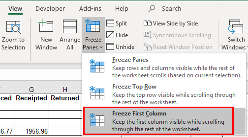
Select View > Freeze Panes > Freeze First Column.
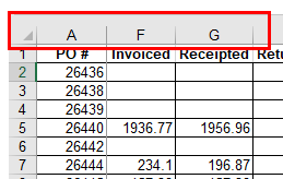
The faint line that appears between Column A and B shows that the first column is frozen.
Freeze the first two columns
-
Select the third column.
-
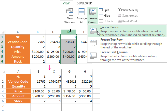
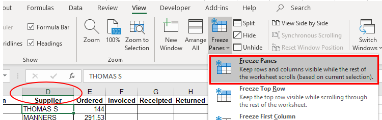
Select View > Freeze Panes > Freeze Panes.
Freeze columns and rows
-
Select the cell below the rows and to the right of the columns you want to keep visible when you scroll.
-
Select View > Freeze Panes > Freeze Panes.
Unfreeze rows or columns
-
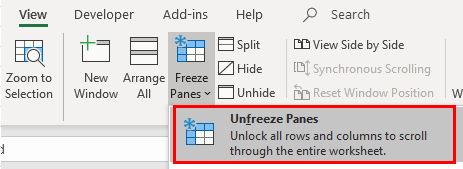
On the View tab > Window > Unfreeze Panes.

Note: If you don’t see the View tab, it’s likely that you are using Excel Starter. Not all features are supported in Excel Starter.

Need more help?
You can always ask an expert in the Excel Tech Community or get support in the Answers community.
See Also
Freeze panes to lock the first row or column in Excel 2016 for Mac
Split panes to lock rows or columns in separate worksheet areas
Overview of formulas in Excel
How to avoid broken formulas
Find and correct errors in formulas
Keyboard shortcuts in Excel
Excel functions (alphabetical)
Excel functions (by category)
Need more help?
Want more options?
Explore subscription benefits, browse training courses, learn how to secure your device, and more.
Communities help you ask and answer questions, give feedback, and hear from experts with rich knowledge.
The column lock feature in Excel is used to avoid any mishaps or undesired changes in data made by mistake by any user. We can apply this feature to a single column or multiple columns at once or separately. After selecting the desired column, change the formatting of the cells from locked to unlocked and password protect the workbook, which will not allow any user to change the locked columns.
For example, suppose we need to allow editing for necessary cells in an Excel spreadsheet but need not want others to edit cells containing essential data such as company information, formulas, drop-down lists, etc. Using this Excel feature, we can protect (lock) specific cells, columns, or rows on our Excel spreadsheet hassle-free and without any extra effort.
Locking a column can be done in two ways. We can do this by using the freeze panes in ExcelFreezing panes in excel helps freeze one or more rows and/or columns so that they remain fixed while scrolling through the database.read more and by protecting the worksheet by using the review functions of Excel. In Excel, we may want to lock a column so that the column does not disappear in case the user scrolls the sheet. That mainly happens when we have a large count of headers in a single sheet, and the user needs to scroll the sheet to see the other information.
When the user scrolls the data, some columns may lapse and not be visible to the user. So, we can lock the columns from getting scrolled out for the visible area.
Table of contents
- Excel Column Lock
- How to Lock Column in Excel?
- #1 – Locking the First Column of Excel
- #2 – Lock any other Column of Excel
- #3 – Using the Protect Sheet Feature to Lock a Column
- Explanation of Column Lock in Excel
- Things to Remember
- Recommended Articles
- How to Lock Column in Excel?
How to Lock Column in Excel?
#1 – Locking the First Column of Excel
Let us start.
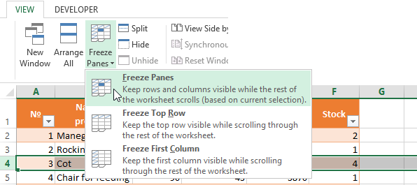
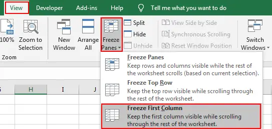
- We must go to the View tab from the ribbon and choose the option of Freeze Panes.

- From the Freeze Panes options, choose the option of Freeze First Column.
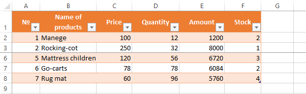
As a result, this will freeze the first column of the spreadsheet.


#2 – Lock any other Column of Excel
If the column is to be locked, we need to follow the below steps.
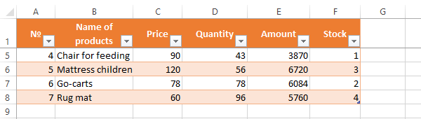
- Step #1 – We must select the column that needs to be locked. If we want to lock column “D,” we must choose the “E” column.

- Step #2 – From the “View” tab, we must choose the “Freeze Pane” option and select the first option to lock the cell.

The output is shown below:

#3 – Using the Protect Sheet Feature to Lock a Column
In this case, the user will not be able to edit the content of the locked column.
- Step #1 – Select the complete sheet and change the “Protection” to unlocked cells.

- Step #2 – Now, we must select the column that we want to lock and change the property of that cell to “Locked.”

- Step #3 – We must go to the “Review” tab and click on the “protect sheetWhen we don’t want any other user to make changes to our worksheet, we can use the Protect worksheet feature in Excel. It can be found in Excel’s Review tab. read more,” and then click on “OK.” Now, it will lock the column.


Explanation of Column Lock in Excel
Have you ever wondered what will happen if someone changes the value of a cell or a complete column? Yes, this may happen, especially in cases where the sheet is shared with multiple team users.
If this happens, this may drastically change the sheet’s data, as many other columns may depend upon the values of another column.
So, if we share our file with other users, we must ensure that the column is protected and no user can change the value of that column. We can do this by protecting the columns and hence locking their columns. If we lock a column, we can choose to have a password to unlock a column or prefer to continue without a password.
It is about locking the column, but sometimes we want a specific column that does not lapse in case the sheet is scrolled and always visible on the sheet.
In this case, we need to use the “Freeze Panes” option in Excel. Using this option, we can fix the position of a column. As a result, this position does not change even if the sheet is scrolled. Using the freeze panes, we can lock the first column, any other column, or even lock the rows and columns of ExcelA cell is the intersection of rows and columns. Rows and columns make the software that is called excel. The area of excel worksheet is divided into rows and columns and at any point in time, if we want to refer a particular location of this area, we need to refer a cell.read more.
Things to Remember
- If we lock a column using the “Freeze Panes” option, only the column is locked from scrolling, and we can always change the column’s content anytime.
- If we are using the “Protect Sheet” and the “Freeze Panes” options, then it is only possible to protect the column’s content and protect it from scrolling.
- If we want a column that is not the first column to freeze, we need to select the next right column, and then we need to click on “Freeze Panes.” Hence, we should always choose the next column to freeze the previous column.
- We can choose to have a password if we protect a column or continue without a password.
Recommended Articles
This article is a guide to Excel Column Lock. We discuss column lock in Excel using freeze panes, examples, and a downloadable Excel template. You may also learn more about Excel from the following articles: –
- Protect Sheet in VBA
- Compare and Match Excel Columns
- Excel Column to Number
- Freezing Excel Cell
- Trunc in Excel
Excel Column Lock (Table of Contents)
- Lock Column in Excel
- How to Lock Column in Excel?
Lock Column in Excel
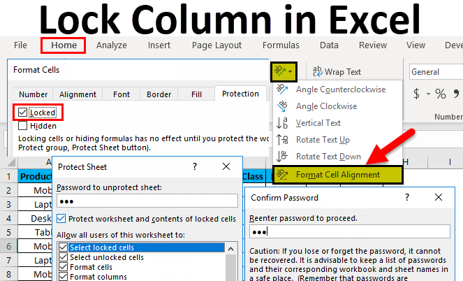
To lock a column in Excel, we first need to select the column we need to Lock. Then click right anywhere on the selected column and select the Format Cells option from the right-click menu list. Now from the Protection tab of Format Cells, check the box of LOCKED with a tick. There is another way to lock a column which can be done using the Protect Sheet option available under the Review menu tab. First, select the column which wants to lock, then use Protect Sheet with a password to lock it.
How to Lock Column in Excel?
To Lock a column in excel is very simple and easy. Let’s understand how to Lock Columns in Excel with some examples.
You can download this Lock Column Excel Template here – Lock Column Excel Template
Example #1
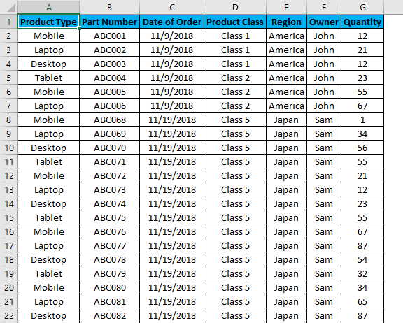
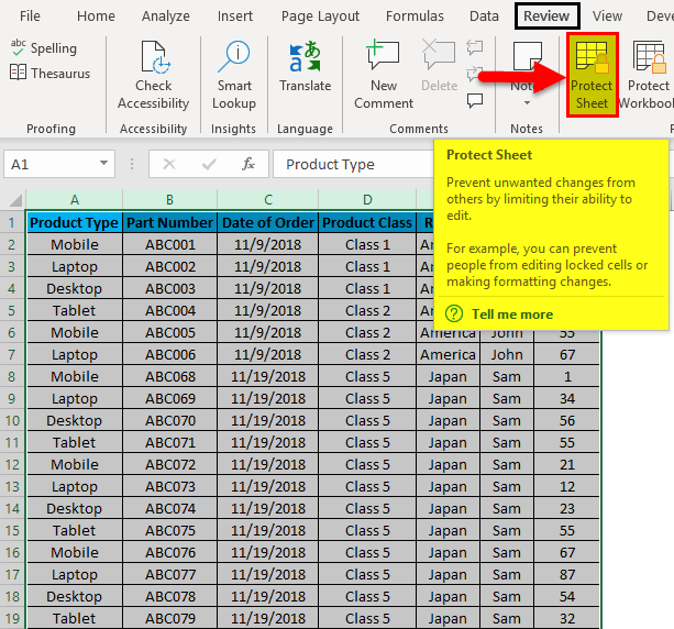
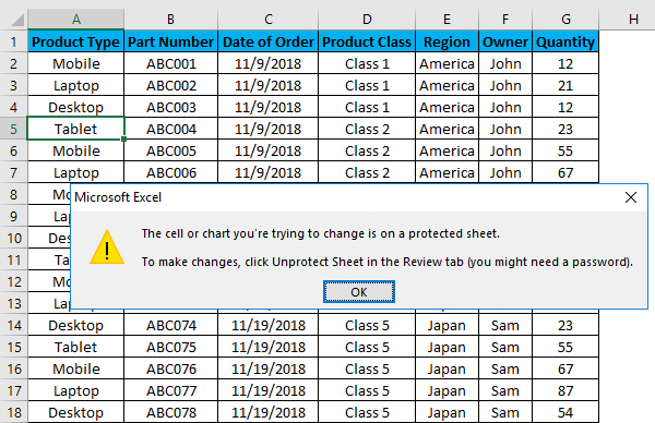
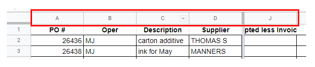
We got sample sales data from some products. Where we have observed that the Product Type column many times got changed by multiple logins. So, to avoid this, we are going to lock that Product Type column so that no one will change it. And data available after it will be accessible for changes. Below is the screenshot of available data for locking the required column.
- For this purpose, first, select a cell or column which we need to protect, and then go to the Review tab and click on Protect Sheet.
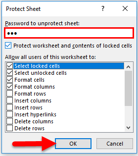
- Once we click on Protect Sheet, we will get a dialog box of Protect Sheet where we need to set a Password of any digit. Here we have set the password as 123.
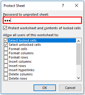
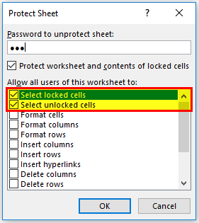
- And check (tick) the options available in a box as per requirement. For example, I have checked selective locked cells and selected unlocked cells (which sometimes comes as default).
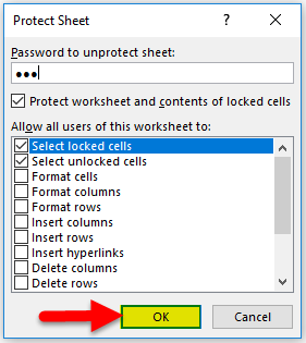
- Once we are done with selecting the options for protecting the sheet or column, click on OK as highlighted below.
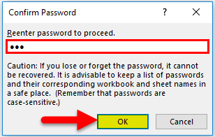
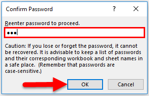
- Once clicked on OK, the system will ask you to re-enter the password again. Once fed the password, click OK.
Now selected Column is locked, and no one can change anything in it without disabling the column’s protection.
Let’s check whether the column is actually protected now. We had chosen Column A named as Product Type as required. For checking it, try to go in edit mode for any cell of that column (By Pressing F2 or double click); if it is protected, we will see a warning message as below.
Hence, our column data is now protected successfully.
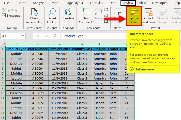
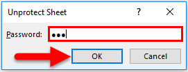
For unprotecting it again, go to the Review tab and click on the Unprotect Sheet, as shown below.
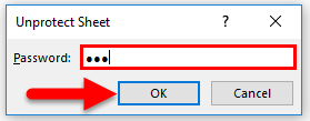
Once we click on the Unprotect Sheet, it will again ask for the same password to unprotect it. For that, re-enter the same password and click on Ok.
Now the column is unprotected, and we can make changes to it. We can also check the column whether it is accessible or not.
Example #2
Apart from the method which we have seen in the above example, we can lock any column in excel by this too. In this method, we will lock the desired column by using the Format Cell in Excel. If you are using this function for the first time, you will see your entire sheet selected as Locked to check-in Format cell. For that, select the entire sheet and go to the Home menu and Click the Orientation icon as shown below.
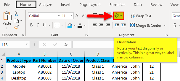
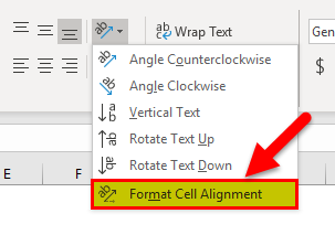
After that, a drop-down will appear. From there, click on Format Cell Alignment, as shown below.
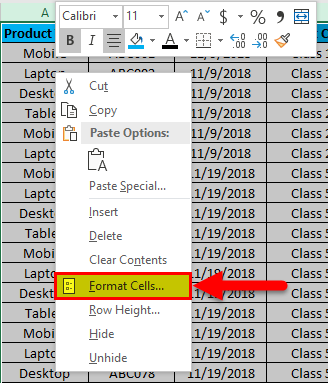
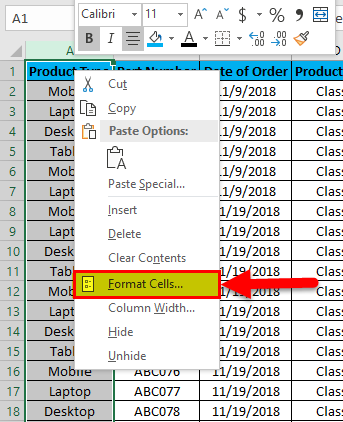
Format Cell Alignment can be accessed from different methods as well. This one is a shortcut approach for doing it. For this, select the entire sheet and Right Click anywhere. We will have the Format Cells option from right-click menu, as shown in the below screenshot. Click on it.
Once we click on it, we will get a dialog box of Format Cell. From there, go to the Protection tab.
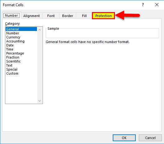
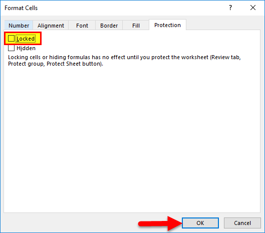
If you find the Locked box is already checked in (which is the default set), then uncheck it click on OK as shown below.
By doing this, we are clearing the default setting and customizing the sheet/column to protect it. Now select the column which we want to lock in excel. Here we are locking column A named as Product Type. Right-click on the same column, and select the Format Cell option.
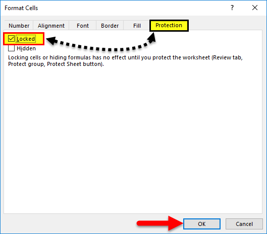
After that, we will see the Format Cell box; go to the Protection Tab and Check-in Locked box. And again, click on OK, as shown below.
Follow the same procedure as explained in example-1. Refer to the below screenshot.
Re-enter the password and click on Ok.
For checking, we already chosen Column A named as Product Type as most of the time, the data available in Product Type gets disturbed. If it is protected, we will see a warning message as below.

So, we will have our column data protected and locked for making any changes.
For unprotecting it again, follow the same procedure as explained in example-1, as shown below.

Once we click on the Unprotect Sheet, it will again ask for the same password to unprotect it. For that, re-enter the same password and click on OK.
Now the column is unprotected, and we can make changes to it. We can also check the column whether it is accessible or not.
Pros of Excel Column Lock
- It helps in data protection by not allowing any unauthorized person to make any changes.
- Sometimes data is so confidential that, even if a file is shared with someone outside the company, then also a person will not be able to do anything, as the sheet/column is locked.
Cons of Excel Column Lock
- Sometimes sheet gets so locked that, even in an emergency, we would not be able to change anything.
- If we forget the password, then also there is no way to make changes in data. There will be only one way to create a new file with the same data to proceed further.
Things to Remember
- Always note the password if you cannot remember it in the long future use.
- Always have a backup of the file which is locked, without any password, so that it will be used further.
- There are no criteria for creating a password.
Recommended Articles
This has been a guide to Lock Column in Excel. Here we discuss how to Lock Columns in Excel along with practical examples and a downloadable excel template. You can also go through our other suggested articles –
- Excel Lock Formula
- COLUMNS Formula in Excel
- VBA Columns
- Switching Columns in Excel
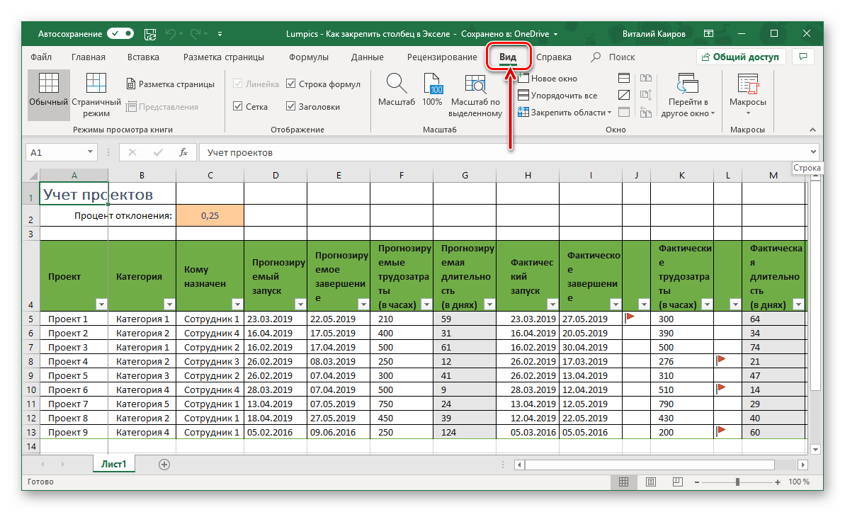
The Microsoft Excel program is designed not only to enter data into the table conveniently and edit it as you need it, but also to view large blocks of information. Most people using PCs work with it constantly.
The columns and rows names can be significantly removed from the cells with which the user is working at this time. Scrolling the page to see the name of the document is not comfortable for any user. Therefore, the Tabular Processor has possibilities to fix certain areas.
Locking a row in Excel while scrolling
Usually an Excel table has one cap. Meanwhile, this document can have up to thousands of rows. Working with multipage table blocks is inconvenient when column names are not visible. Scrolling the page to its beginning to return to the correct cell is absolutely irrational. To make the cap visible when scrolling, fix the top row of the Excel table, following these actions:
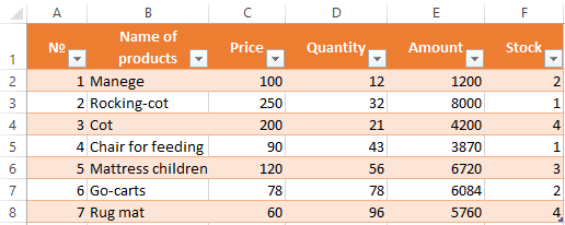
- Create the needed table and fill it with the data.
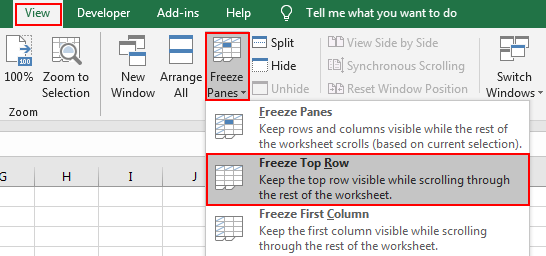
- Make any of the cells active. Go to the “VIEW” tab using the tool “Freeze Panes”.
- In the menu select the “Freeze Top Row” functions.
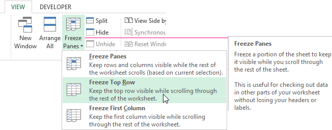
You will get a delimiting line under the top line. Now when you scroll vertically the table cap will be always visible.
Locking several rows in Excel while scrolling
Let us suppose, a user needs to fix not only the cap. For instance, another row or even a couple of rows must be fixed when scrolling the document. Doing it is possible and easy, when you follow these steps:
- Select any cell under the line, which we will fix. This action will help Excel to “understand”, which area should be fixed;
- Now select the “Freeze Panes” tool.
When you perform horizontal and vertical scrolling, the cap and the top row of the table remain fixed. Thus, you can fix two, three, four and more rows.
Note: This method works for 2007 and 2010 Excel versions. In earlier versions the “Lock areas” tool is located in the “Window” menu on the main page. There you must always (!) activate the cell under the freeze row.
Freezing columns in Excel
For instance, the information in the table has a horizontal direction. It is not concentrated in columns, but located in rows. For his comfort, the user must freeze the first column, containing the lines’ names in horizontal scrolling.
- Select any cell of the chosen table so that Excel understands with what data it will work. Pin the first column in the menu you will see..
- Now, when the document is scrolled to the right horizontally, the needed column will be fixed.
To freeze several columns, select the cell at the page bottom (to the right from the fixed column). Pick the “Freeze Panes” button.
How to freeze the row and column in Excel
You have a task – to freeze the selected area, which contains two columns and two rows.
Make a cell at the intersection of the fixed rows and columns active. However, the cell must be not placed in the fixed area. It should have the position right under the required lines (to the right of the required columns). Pick the first option in Excel Locking Areas. The photo shows that when scrolling, the selected areas remain at the same place.
Removing a fixed area in Excel
After fixing a row or a column of the table the button deleting all pivot tables becomes available.
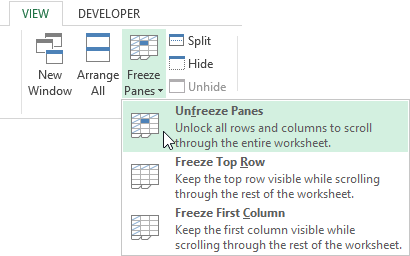
After clicking – «Unfreeze Panes», all the locked areas of the worksheet become unlocked.
How To Lock Columns In Excel
This element within Excel allows others to enter or edit information into all other cells except those locked. Hiding or locking cells has no effect at all on the Worksheet until you protect the Worksheet.
When sharing projects among several team members, sometimes it is necessary to lock certain cells within the Worksheet to ensure the data isn’t deleted or changed. When the Worksheet is shared, the team member will be able to adjust all unlocked cells; however, the locked cells will remain the same.
The Worksheet Has Already Been Protected
If the Worksheet has already been protected, the first step is to unprotect it by clicking the REVIEW tab within the Ribbon and selecting Unprotect Sheet. You might have to enter a password if the Worksheet was protected with one originally.

- Select the whole Worksheet by clicking on the select all arrow in the top left of the Worksheet (highlighted in the picture above).
- Right-click anywhere and select FORMAT CELLS from the menu options or from the HOME Tab to click the small arrow at the bottom right of the Font box, or you can simply enter (Control + Shift + F) to have the Format Cells box open.
- In the PROTECTION Tab of the Format Cells box, uncheck Lock Cells and click OK to complete unlock all cells within the Worksheet so you can designate the specific cells within the Worksheet that you want to lock.

- Now, back on the Worksheet, select the column(s) that you would like to Lock. Open the Format Cells box again and this time click to put a checkmark back in the Locked checkbox.
- Go back to the REVIEW tab and select PROTECT THIS WORKSHEET.
- A dialog box will pop up asking if you would like to password protect the Worksheet, and there are numerous elements that you can either allow or disallow users to do within the Worksheet. The first two elements are selected by default:
- Select lock cells – allow users to select cells that are locked but do not allow changes or deletion
- Select unlock cells – allow users to select and make changes within all unlocked cells.
- All other elements are related to formatting, sorting, inserting/deleting columns and rows, and not selecting by default.

Once you click OK, the Worksheet will now be protected.
- If someone attempts to make changes into a locked cell, the following message will pop up on the screen.


How To Lock Columns In Excel To Unlock Columns
You will need to begin by un-protecting the Sheet under the Review tab. Select the column you have locked and bring up the Format Cells box. Under the PROTECTION tab once again, unclick the Locked checkbox.
How To Lock Columns In Excel
Locking cells could also be beneficial at a networking event where each member could enter their information into a worksheet as shown to the left. Column A could be locked in place to ensure that no changes are made; however, members could easily enter their information under each column.
See all How-To Articles
This tutorial demonstrates how to lock columns so they stay in view as you scroll in Excel and Google Sheets.
Freeze Left Column
If you have a large worksheet with many columns going across the screen, you might want to make sure that you can always see the first column.
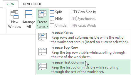
- In the Ribbon, select View > Freeze Panes.
- Select Freeze First Column.
As you scroll in the worksheet, you can see that the first column remains visible regardless of how far you scroll across.
- To remove the pane freeze, select Unfreeze Panes from the Freeze Panes menu.
Freeze Panes
You can freeze more than one column with Freeze Panes.
- Position your cursor in the column you wish to freeze.
- In the Ribbon, select View > Freeze Panes > Freeze Panes.
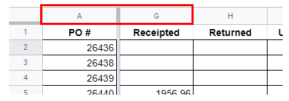
The worksheet freezes Columns A to C. If you scroll across, these columns remain in place.
- To remove the pane freeze, select Unfreeze Panes from the Freeze Panes menu.
Freeze First Column in Google Sheets
- In the Menu, click View > Freeze > 1 column.
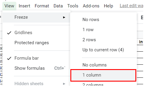
As you scroll across, the left column remains in place.
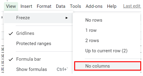
- Click View > Freeze > No columns to remove the freeze.
To freeze more than one column in Google Sheets, you can select either 2 columns to freeze the top two columns, or Up to current column(col) to freeze up to the column you have selected.

Note that the letter in parentheses after Up to current column reflects the column you have selected.
You can also use Freeze Panes to freeze rows.
Were you looking instead for how to lock cell references in formulas or how to lock cells for editing with a password?
Suppose we create a large table in excel spreadsheet and it lists large amount of data. There are headers in the first row, and if we want to drag the scroll bar to view the bottom of table, the headers are hidden due to it lists on the top. So, in this case if we want to see the headers all the time, we need to freeze the first row to make it fixed and always displays on the top even we drag the scrollbar. On the other side, sometimes we need to freeze more rows, or columns, or even freeze row and column simultaneously. To implement this, we need to know the way to freeze row and columns. This article will introduce different ways to freeze row and columns with examples for you, you can’t miss it.
Table of Contents
- Method 1: How to Freeze the First Row in Excel Spreadsheet
- Method 2: How to Freeze Multiple Rows in Excel Spreadsheet
- Method 3: How to Freeze the First Column in Excel Spreadsheet
- Method 4: How to Freeze Row and Column in Excel Spreadsheet
- Method 5: How to Freeze Rows and Columns in Excel Spreadsheet
Method 1: How to Freeze the First Row in Excel Spreadsheet
In most daily work, freeze the first row in table is frequently needed due to in most tables the first row lists the headers. So, people always want to see the headers on top no matter whether they drag the scrollbar to the end or not. See example below:
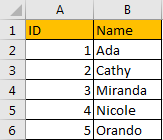
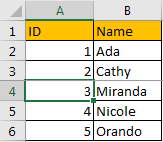
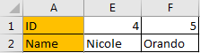
Suppose it lists a long list of ID and names. Header ID and Name are listed on the top. Now let’s freeze the first row.
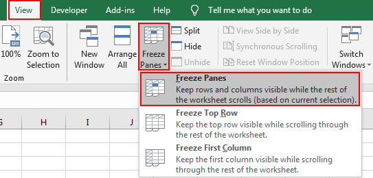
Step 1: Click View in the ribbon, then click Freeze Panes in Window group, then click the small triangle of Freeze Panes to load below three options, select the middle one ‘Freeze Top Row’.
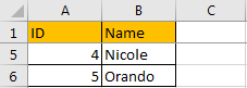
Step 2: After above operating. The first top row is fixed and always displayed on the top. Try to drag the scrollbar. You can see the header row is stayed on the top.
Method 2: How to Freeze Multiple Rows in Excel Spreadsheet
If you want to freeze the first three rows in excel, you can just select the first cell in the fourth row, then freeze the rows above the selected cell. See details below.
Step 1: Click A4 in the table.
Step 2: Click View in the ribbon, then click Freeze Panes in Window group, then click the small triangle of Freeze Panes to load below three options, select the first one ‘Freeze Panes’.
Step 3: Try to drag the scrollbar. Verify that top three rows are fixed.
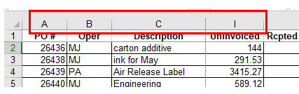
Method 3: How to Freeze the First Column in Excel Spreadsheet
See screenshot below:
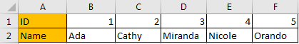
Now let’s freeze the first column. The way is similar with freeze the first row.
Step 1: Click View in the ribbon, then click Freeze Panes in Window group, then click the small triangle of Freeze Panes to load below three options, select the middle one ‘Freeze First Column’.
Step 2: Verify if it works well.
Obviously, it works.
Method 4: How to Freeze Row and Column in Excel Spreadsheet
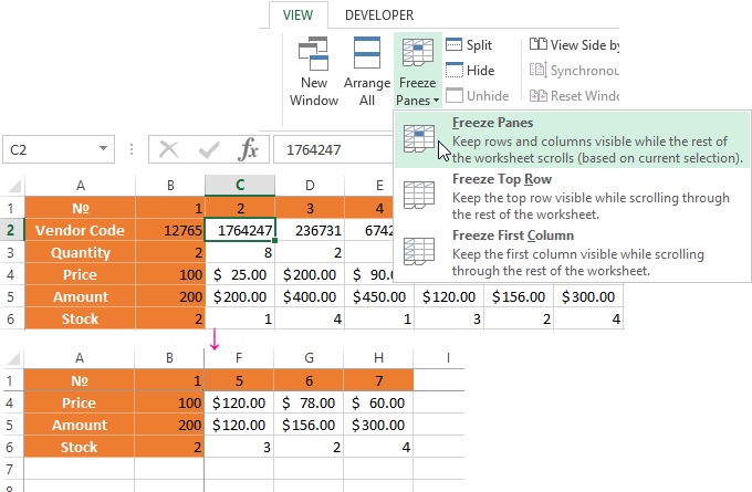
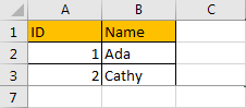
If you want to just freeze the first row and column, just click on B2. Then click View->Freeze Panes->Freeze Panes in Window group.

Method 5: How to Freeze Rows and Columns in Excel Spreadsheet
If you want to freeze multiple rows and columns, refer to the description of Freeze Panes ‘Keep rows and column visible while the rest of the worksheet scrolls (based on current selection)’ we can know that we can select a cell to make it as the first cell outside of your fixed area. For example, if we want to freeze the top three rows and first two columns (row 4 is not fixed and column C is not fixed), we can click on C4, then repeat above steps to freeze panes.
As an Excel user, you may have come across the term “column lock” while working with your spreadsheet. But do you really understand what it means and how it can be useful in your work? In this comprehensive guide, we’ll delve deep into the concept of column lock in Excel and how you can use it to your advantage.
What is Column Lock in Excel?
Column lock in Excel refers to the ability to freeze or lock specific columns in place while scrolling through the rest of the spreadsheet. This is especially useful when you have a large spreadsheet with multiple columns, and you want to keep certain columns visible at all times while you scroll through the data.
For example, let’s say you have a spreadsheet with customer data, including their names, addresses, and purchase history. If you want to keep the customer names visible while scrolling through the rest of the data, you can use column lock to freeze the first column in place. This way, you can easily reference the customer names as you work with the rest of the data.
The picture might show four screens, each representing a different version of Excel (Windows, Mac, web, and mobile). Each screen would have a spreadsheet open, with certain columns locked in place. The locked columns might be highlighted in a different color or marked with a lock icon to indicate that they are frozen. The other columns on each screen would be scrollable, allowing the user to view the rest of the data.
How to Lock Columns in Excel
Now that you understand the concept of column lock let’s take a look at how you can lock columns in Excel. There are a few different ways to do this, depending on your preferences and the version of Excel you’re using.
Method 1: Freeze Panes
One of Excel’s most common methods for locking columns is using the “Freeze Panes” feature. This method allows you to freeze both rows and columns simultaneously.
Here’s how to use the Freeze Panes feature:
- Open your Excel spreadsheet and navigate to the cell where you want to split the frozen and unfrozen areas. For example, if you want to freeze the first column, navigate to cell B2.
- Click on the “View” tab in the ribbon at the top of the screen.
- In the “Window” group, click on the “Freeze Panes” dropdown arrow.
- Select the “Freeze Panes” option.
Your columns should now be frozen in place. You can scroll through the rest of the spreadsheet while the frozen columns remain visible.
Method 2: Split Feature
Another method for locking columns in Excel is using the “Split” feature. This method allows you to split the screen into separate panes, with each pane containing its own set of rows and columns. You can then freeze one or more panes to keep certain rows or columns visible while you scroll through the rest of the data.
Here’s how to use the Split feature:
- Open your Excel spreadsheet and navigate to the cell where you want to split the screen.
- Click on the “View” tab in the ribbon at the top of the screen.
- In the “Window” group, click on the “Split” button.
- Your screen should now be split into two panes, with a horizontal and vertical split line in the middle. You can click and drag the split lines to adjust the size of the panes.
- To freeze a pane, click on the “View” tab and click on the “Freeze Panes” dropdown arrow. Select the “Freeze Panes” option.
Your columns should now be frozen in place. You can scroll through the rest of the spreadsheet while the frozen columns remain visible.
Method 3: Freeze Top Row
If you only want to freeze the top row of your spreadsheet (for example, if you have a header row with column titles), you can use the “Freeze Top Row” feature. This is a quick and easy way to lock the top row without using the Freeze Panes or Split features.
Here’s how to use the Freeze Top Row feature:
- Open your Excel spreadsheet and navigate to the top row that you want to freeze.
- Click on the “View” tab in the ribbon at the top of the screen.
- In the “Window” group, click on the “Freeze Panes” dropdown arrow.
- Select the “Freeze Top Row” option.
Your top row should now be frozen in place. You can scroll through the rest of the spreadsheet while the top row remains visible.
How to Unlock Columns in Excel
If you’ve previously locked columns in your Excel spreadsheet and want to unlock them, you can use one of the following methods:
- If you used the Freeze Panes or Split features to lock your columns, click on the “View” tab in the ribbon and click on the “Freeze Panes” dropdown arrow. Select the “Unfreeze Panes” option.
- If you used the Freeze Top Row feature to lock your top row, click on the “View” tab in the ribbon and click on the “Freeze Panes” dropdown arrow. Select the “Unfreeze Top Row” option.
Your columns should now be unlocked and you can scroll freely through the entire spreadsheet.
Benefits of Using Column Lock in Excel
So, why should you use column lock in Excel? Here are a few benefits of this feature:
- Improved organization: By keeping certain columns visible at all times, you can better organize and reference your data as you work with it.
- Enhanced readability: Column lock can make reading and understanding your data easier, especially if you have a large spreadsheet with many columns.
- Increased efficiency: With column lock, you can quickly and easily reference important data without having to constantly scroll back and forth. This can save time and improve your overall efficiency.
Advanced Tips for Using Column Lock in Excel
Once you’ve mastered the basics of column lock in Excel, you can take your skills to the next level with these advanced tips:
- Use column lock in combination with filters: If you’re using filters to view specific subsets of your data, you can use column lock to keep your filters visible as you scroll through the rest of the data.
- Lock multiple columns: You’re not limited to locking just one column. You can freeze multiple columns at the same time using the Freeze Panes or Split features.
- Lock both rows and columns: As mentioned earlier, the Freeze Panes feature allows you to lock both rows and columns simultaneously. This can be useful if you have a large spreadsheet with multiple rows and columns you want to keep visible as you scroll.
Frequently Asked Questions (FAQ)
Q: Can I lock columns in all versions of Excel?
A: Yes, column lock is available in all versions of Excel, including Excel for Windows, Excel for Mac, and Excel for the web.
Q: Can I lock columns in a shared spreadsheet?
A: Yes, you can lock columns in a shared spreadsheet. However, remember that other users will not be able to scroll through the locked columns, so it’s important to communicate with your team about any column lock settings you use.

I am studying at Middle East Technical University. I am interested in computer science, architecture, physics and philosophy.
Love,
Cansu
Tags: #ExcelCharts #ExcelDashboard #ExcelFormulas #ExcelFunctions #ExcelTemplates #ExcelTipsAndTricks #ExcelTutorials
Содержание
- Закрепление столбца в таблице Эксель
- Вариант 1: Один столбец
- Вариант 2: Несколько столбцов (область)
- Открепление зафиксированной области
- Заключение
- Вопросы и ответы

В таблицах с большим количеством столбцов довольно неудобно выполнять навигацию по документу, ведь если она в ширину выходит за границы плоскости экрана, для того чтобы посмотреть названия строк, в которые занесены данные, придется постоянно прокручивать страницу влево, а потом опять возвращаться вправо. На эти операции будет уходить дополнительное количество времени. Поэтому для того, чтобы пользователь мог экономить своё время и силы, в программе Microsoft Excel предусмотрена возможность закрепить столбцы. После выполнения данной процедуры левая часть таблицы, в которой находятся наименования строк, всегда будет на виду. Давайте же разберемся, как зафиксировать столбцы в приложении Excel.
Закрепление столбца в таблице Эксель
При работе с «широкой» таблицей может потребоваться закрепить как один, так и сразу несколько столбцов (область). Делается это буквально в несколько кликов, а непосредственный алгоритм выполнения в каждом из двух случаев отличается буквально на один пункт.
Вариант 1: Один столбец
Для того чтобы закрепить крайний левый столбец, можно даже не выделять его предварительно – программа сама поймет, для какого элемента таблицы требуется принять указанное вами изменение.
- Перейдите во вкладку «Вид».
- Разверните меню пункта «Закрепить области».
- Выберите последний вариант в списке доступных опций – «Закрепить первый столбец».

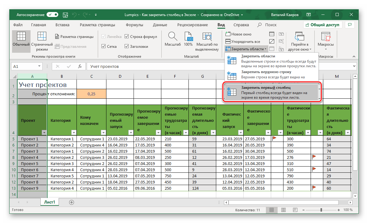
С этого момента при горизонтальной прокрутке таблицы ее первый (левый) столбец всегда будет оставаться на фиксированном месте.
Вариант 2: Несколько столбцов (область)
Бывает и так, что закрепить требуется более одного столбца, то есть область таковых. В данном случае необходимо учесть всего один важный нюанс – не выделяйте диапазон столбцов.
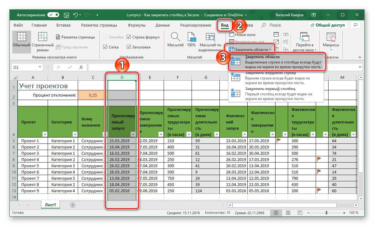
- Выделите столбец, следующий за той областью, которую планируете закрепить. То есть, если требуется закрепить диапазон A-C, выделять необходимо D.
- Перейдите во вкладку «Вид».
- Кликните по меню «Закрепить области» и выберите в нем аналогичный пункт.
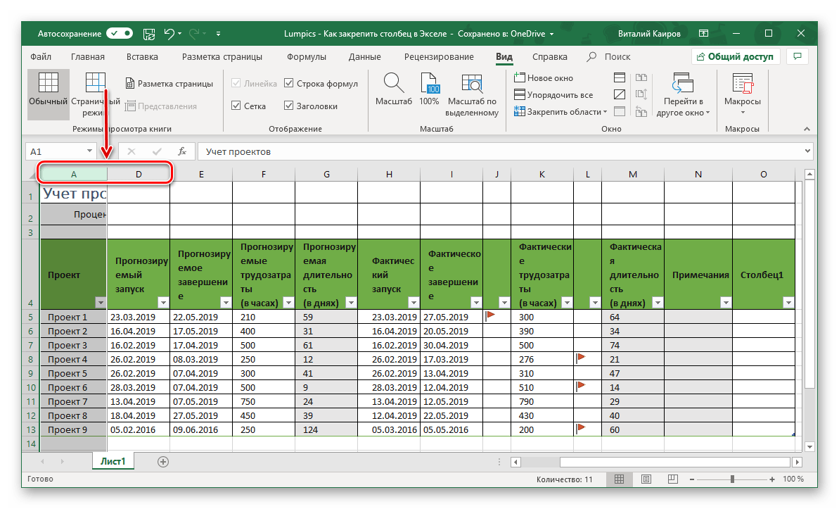
Теперь необходимое вам количество столбцов закреплено и при прокрутке таблицы они будут оставаться на своем месте – слева.

Читайте также: Как в Microsoft Excel закрепить область
Открепление зафиксированной области
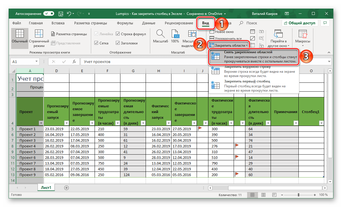
Если необходимость в закреплении столбца или столбцов отпала, во все той же вкладке «Вид» программы Эксель откройте меню кнопки «Закрепить области» и выберите вариант «Снять закрепление областей». Это сработает как для одного элемента, так и для диапазона таковых.
Заключение
Как видите, в табличном процессоре Microsoft Excel можно легко закрепить всего один, крайний левый столбец или диапазон таковых (область). Открепить их, если такая необходимость появится, тоже можно буквально в три клика.
Еще статьи по данной теме: