
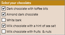
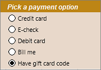
You can insert form controls such as check boxes or option buttons to make data entry easier. Check boxes work well for forms with multiple options. Option buttons are better when your user has just one choice.
To add either a check box or an option button, you’ll need the Developer tab on your Ribbon.
Notes: To enable the Developer tab, follow these instructions:
-
In Excel 2010 and subsequent versions, click File > Options > Customize Ribbon , select the Developer check box, and click OK.
-
In Excel 2007, click the Microsoft Office button
 > Excel Options > Popular > Show Developer tab in the Ribbon.
 > Excel Options > Popular > Show Developer tab in the Ribbon.
-
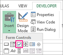
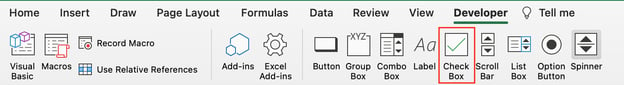
To add a check box, click the Developer tab, click Insert, and under Form Controls, click
.
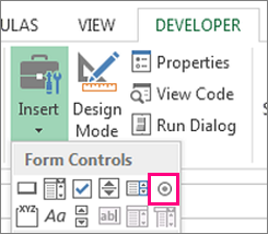
To add an option button, click the Developer tab, click Insert, and under Form Controls, click
.
-
Click in the cell where you want to add the check box or option button control.
Tip: You can only add one checkbox or option button at a time. To speed things up, after you add your first control, right-click it and select Copy > Paste.
-
To edit or remove the default text for a control, click the control, and then update the text as needed.
 .
.
 .
.
Tip: If you can’t see all of the text, click and drag one of the control handles until you can read it all. The size of the control and its distance from the text can’t be edited.
Formatting a control
After you insert a check box or option button, you might want to make sure that it works the way you want it to. For example, you might want to customize the appearance or properties.
Note: The size of the option button inside the control and its distance from its associated text cannot be adjusted.
-
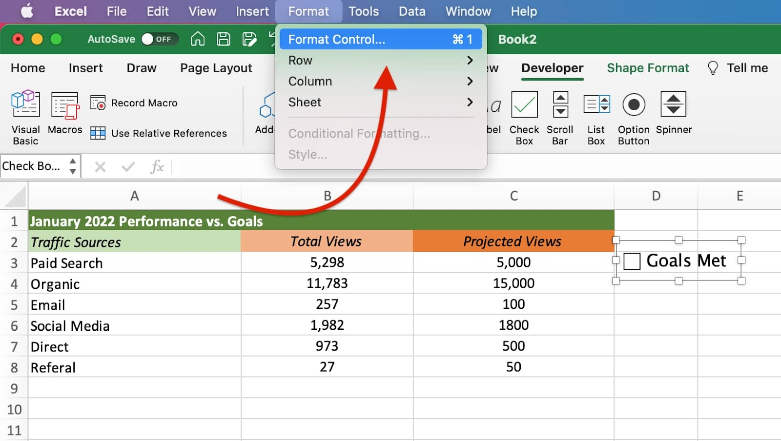
To format a control, right-click the control, and then click Format Control.
-
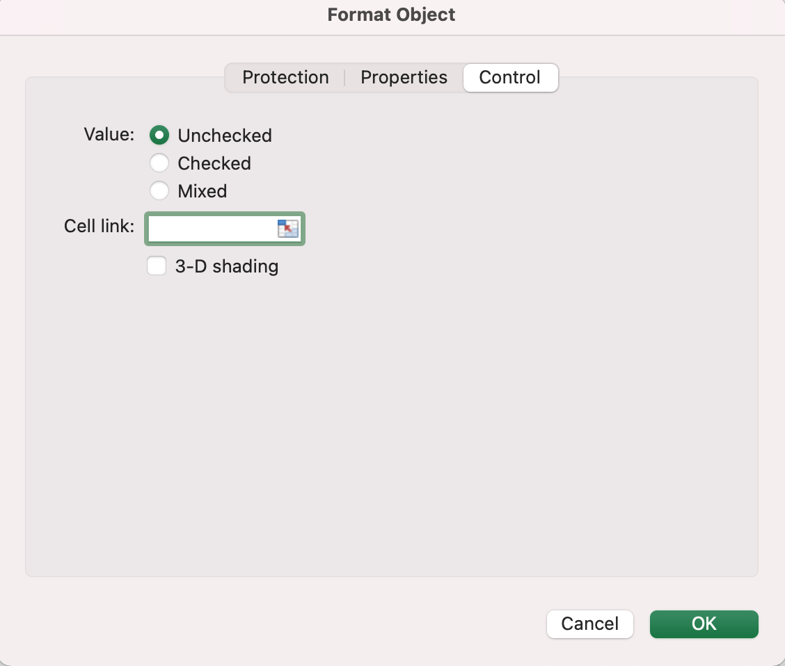
In the Format Control dialog box, on the Control tab, you can modify any of the available options:
-
Checked: Displays an option button that is selected.
-
Unchecked: Displays an option button that is cleared.
-
In the Cell link box, enter a cell reference that contains the current state of the option button.
The linked cell returns the number of the selected option button in the group of options. Use the same linked cell for all options in a group. The first option button returns a 1, the second option button returns a 2, and so on. If you have two or more option groups on the same worksheet, use a different linked cell for each option group.
Use the returned number in a formula to respond to the selected option.
For example, a personnel form, with a Job type group box, contains two option buttons labeled Full-time and Part-time linked to cell C1. After a user selects one of the two options, the following formula in cell D1 evaluates to «Full-time» if the first option button is selected or «Part-time» if the second option button is selected.
=IF(C1=1,»Full-time»,»Part-time»)
If you have three or more options to evaluate in the same group of options, you can use the CHOOSE or LOOKUP functions in a similar manner.
-
-
Click OK.
Deleting a control
-
Right-click the control, and press DELETE.
Currently, you can’t use check box controls in Excel for the web. If you’re working in Excel for the web and you open a workbook that has check boxes or other controls (objects), you won’t be able to edit the workbook without removing these controls.
Important: If you see an «Edit in the browser?» or «Unsupported features» message and choose to edit the workbook in the browser anyway, all objects such as check boxes, combo boxes will be lost immediately. If this happens and you want these objects back, use Previous Versions to restore an earlier version.
If you have the Excel desktop application, click Open in Excel and add check boxes or option buttons.
Watch Video – How to Insert and Use a Checkbox in Excel
In Excel, a checkbox is an interactive tool that can be used to select or deselect an option. You must have seen it in many web form available online.
You can use a checkbox in Excel to create interactive checklists, dynamic charts, and dashboards.
This Excel tutorial covers the following topics:
- How to Get the Developer Tab in Excel Ribbon.
- How to Insert a Checkbox in Excel.
- Examples of Using Checkboxes in Excel.
- How to Insert Multiple Checkboxes in Excel.
- How to Delete a Checkbox in Excel.
- How to Fix the Position of a Checkbox in Excel.
- Caption Name Vs. Backend Name
To insert a checkbox in Excel, you first need to have the Developer tab enabled in your workbook.
Can’t see the developer tab?
Don’t worry and keep reading!
Get the Developer Tab in Excel Ribbon
The first step in inserting a checkbox in Excel is to have the developer tab visible in the ribbons area. The developer tab contains the checkbox control that we need to use to insert a checkbox in Excel.
Below are the steps for getting the developer tab in the Excel ribbon.
Now with the Developer tab visible, you get access to a variety of interactive controls.
Here are the steps to insert a checkbox in Excel:
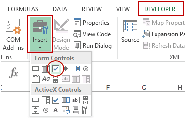
- Go to Developer Tab –> Controls –> Insert –> Form Controls –> Check Box.

- Click anywhere in the worksheet, and it will insert a checkbox (as shown below).

- Now to need to link the checkbox to a cell in Excel. To do this, right-click on the checkbox and select Format Control.

- In the Format Control dialog box, in the Control tab, make the following changes:
- Value: Checked (this makes sure that the checkbox is checked by default when you open the workbook)
- Cell Link: $A$1 (this is the cell linked to the checkbox). You can manually enter this or select the cell to get the reference.

- Click OK.


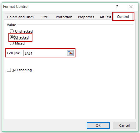
Now your checkbox is linked to cell A1, and when you check the checkbox, it will show TRUE in cell A1, and when you uncheck it, it will show FALSE.

Examples of Using a Checkbox in Excel
Here are a couple of examples where you can use a checkbox in Excel.
Creating an Interactive To-Do List in Excel
Below is an example of a To-Do list that uses checkboxes to mark the task as complete.
A couple of things are happening in the example above:
- As soon as you check the checkbox for an item/task, the status changes to Done (from To be Done), the cell gets a green shade, and the text gets a strikethrough format.
- The value of the cell link for that checkbox changes from FALSE to TRUE.
- The ‘Task Completed’ and ‘% of Task Completed’ numbers (in cell H3 and H4) change based on how many tasks have been marked as completed.
Here is how to make this:
- Have the activities listed in cell A2:A7.
- Insert checkboxes and place it in cell B2:B7.
- Link these checkboxes to cell E2:E7. There is no way to link all the checkboxes at one go. You’ll have to manually link each checkbox one by one.
- In cell C2, enter the following formula: =IF(E2,”Done”,”To Be Done”) and drag for all the cells (C2:C7).
- In cell C2:C7, apply conditional formatting to give the cell a green background color and strikethrough format when the value in the cell is Done.
- In cell H3, use the following formula: =COUNTIF($E$2:$E$7,TRUE)
- This will count the total numbers of tasks that have been marked as completed.
- In cell H4, use the following formula: =COUNTIF($E$2:$E$7,TRUE)/COUNTIF($E$2:$E$7,”<>”)
- This will show the percentage of tasks completed.
Click here to download the checklist.

Creating a Dynamic Chart in Excel
You can use an Excel checkbox to create a dynamic chart as shown below:
In this case, the checkbox above the chart is linked to cell C7 and C8.
If you check the checkbox for 2013, the value of cell C7 becomes TRUE. Similarly, if you check the checkbox in for 2014, the value of cell C8 becomes TRUE.
The data used in creating this chart is in C11 to F13. The data for 2013 and 2014 is dependent on the linked cell (C7 and C8). If the value in cell C7 is TRUE, you see the values in C11:F11, else you see the #N/A error. Same is the case with data for 2014.
Now based on which checkbox is checked, that data is shown as a line in the chart.
Click here to download the dynamic chart template.
Inserting Multiple Checkboxes in Excel
There are a couple of ways you can insert multiple checkboxes in the same worksheet.
#1 Inserting a Checkbox using the Developer Tab
To insert more than one checkbox, go to the Developer Tab –> Controls –> Insert –> Form Controls –> Check Box.
Now when you click anywhere in the worksheet, it will insert a new checkbox.
You can repeat the same process to insert multiple checkboxes in Excel.
Note:
- The checkbox inserted this way are not linked to any cell. You need to manually link all the checkboxes.
- The checkbox would have different caption names, such as Check Box 1 and Check Box 2, and so on.
#2 Copy Pasting the Checkbox
Select an existing checkbox, copy it and paste it. You can also use the keyboard shortcut (Control + D).
Note:
- The copied checkboxes are linked to the same cell as that of the original checkbox. You need to manually change the cell link for each checkbox.
- The caption names of all the copied checkboxes are the same. However, the backend name would be different (as these are separate objects).
#3 Drag and Fill Cells with Checkbox
If you have a checkbox in a cell in Excel and you drag all fill handle down, it will create copies of the checkbox. Something as shown below:

Note:
- The caption names of all the new checkboxes are the same. However, the backend name would be different (as these are separate objects).
- All these checkboxes would be linked to the same cell (if you linked the first one). You need to manually change the link of all these one by one.
Deleting the Checkbox in Excel
You can easily delete a single checkbox by selecting it and pressing the delete key. To select a checkbox, you need to hold the Control key and the press the left button of the mouse.
If you want to delete multiple checkboxes:
- Hold the Control key and select all the ones that you want to delete.
- Press the Delete key.
If you have many checkboxes scattered in your worksheet, here is a way to get a list of all the checkbox and delete at one go:
Note: The selection pane displays all the objects of the active worksheet only.
How Fix the Position of a Checkbox in Excel
One common issue with using shapes and objects in Excel is that when you resize cells or hide/delete rows/columns, it also affects the shapes/checkboxes. Something as shown below:

To stop the checkbox from moving around when you resize or delete cells, do the following:
Now when you resize or delete cells, the checkbox would stay put.
Caption Name Vs. Name
When you insert a checkbox in Excel, you see a name in front of the box (such as Check Box 1 or Check Box 2).
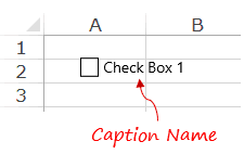
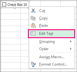
This text – in front of the box – is the Caption Name of the checkbox. To edit this text, right-click and select the ‘Edit Text’ option.

While you see the new text, in the backend, Excel continues to refer to this checkbox as Check Box 1.
If you select the checkbox and look at the Name Box field, you will see the name Excel uses for this checkbox in the backend.
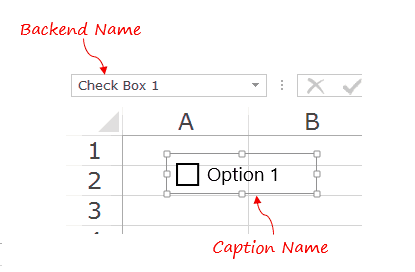
You can easily change this backend name by first selecting the checkbox in the worksheet and then typing the name in the name box (the naming rules are same as that of named ranges).
See Also: How to Insert a Checkbox in Google Sheets.
You May Also Like the Following Excel Tutorials:
- Inserting Checkmark in Excel.
- Create Dynamic Chart using Checkbox.
- Create Checklists using Checkbox in Excel.
- VBA Guide to Using Checkboxes in Excel.
- How to Insert a Scroll Bar in Excel.
- How to Insert and Use a Radio Button in Excel.
Inserting a checkbox in Excel is an easy task. The checkbox control is available in the Excel developer tools option. Checkbox and other controls like dropdowns can be quite helpful while designing forms in Excel.
These controls prevent users from entering some unwanted data in your forms, and hence they are preferred.
In this post, we will understand how to insert a checkbox in Excel. After that, we will also see an example of how checkboxes can ease data analysis tasks. 1")
How to Insert a Checkbox in Excel
Excel checkbox control is present in the «Developer Tools» menu item. And by default «Developer Tools» menu item is hidden in Excel. So first of all, we need to make this option available in the Excel top ribbon, and after that, we can use the checkbox control. Below is a step by step procedure for adding a checkbox to Excel:
- Navigate to Excel Options > Customize Ribbon: With the Excel sheet opened, navigate to «File»> «Options»> «Customize Ribbon» tab. You can also press the keys «ALT + F + T» to open the excel options and then navigate to the «Customize Ribbon» tab.
 2")
- Enable Developer Tools Tab: By default, «Developer» option would be unchecked in the «Main Tabs». Check the «Developer» option and click the «OK» button.
- Go to Developer Tab > Insert Option > Checkbox Option: After this, you will be able to see a «Developer» tab on your Excel ribbon. Inside the «Developer» tab, click on the «Insert» dropdown and select the form «Checkbox» control as shown.
 3")
- Click the Checkbox Option: Now, you can draw a checkbox anywhere on your excel sheet.
- Format Checkbox Control: Next, you can customize your checkbox using the «Format Control» option.
How to Capture the Checkbox State
After adding the checkbox to your spreadsheet, you need to capture its state. Checkbox state can tell you if the checkbox is currently checked or not.
For capturing the state of a checkbox, you need to associate it with a cell. After associating the checkbox with a cell, the cell displays ‘True’ if the checkbox is checked; otherwise, it displays ‘False’.
To associate checkbox to a cell, follow the below steps:
- Right-click over the checkbox and select the option ‘Format Control’ from the context menu as shown.
 4")
- Clicking on the ‘Format Control’ option will open a ‘Format Control’ window. Inside the ‘Format Control’ window navigate to the ‘Control’ tab.
 5")
- On the control tab, click on the ‘cell link’ input box and then select an empty cell on the spreadsheet which you wish to associate with the checkbox.
 6")
Tip: To keep track of the cell links for corresponding checkboxes, it’s always a good idea to set the cell links in a column adjacent to the checkbox. This way, it gets easier to find the cell links associated with the checkboxes whenever you want. Also, you can hide the column containing the cell links so that your spreadsheet is clutter-free.
How To Insert Multiple Checkboxes Fast in Excel
In the above sections, we saw, how to add a single checkbox to excel, but there can be times where you would need to have tens or hundreds of checkboxes in your worksheet. Adding such a huge number of checkboxes on by one is not a feasible option.
So, let’s see how can we add multiple checkboxes to excel fast:
- First of all, add a checkbox manually, by selecting the checkbox option from the Developer tab.
 7")
- Next, adjust the position of the checkbox.
 8")
- Optional Step: Format the checkbox as required. In this example, we are setting the checkbox text as blank.
 9")
- After this, right-click over the checkbox and select the ‘Format Control’ option from the context menu.
 10")
- In the ‘Format Control’ window, navigate to the ‘Properties’ tab and check if the option «Move but don’t size cells» option is selected. If this option is not selected, select it and click the «OK» button.
 11")
- Finally, when the check box is positioned correctly and formatted correctly. Drag the fill handle to all the rows below.
 12")
- And it’s done! Now you will see checkboxes copied against all the rows.
 13")
As you can see in the screenshot above, we have inserted checkboxes for all the rows in our list. But the list cannot be used as such, because we still haven’t set the cell links for all those checkboxes. Now let’s see how to add cell links for multiple checkboxes.
Setting the Cell Link for Multiple Checkboxes
Setting cell links for multiple checkboxes manually can become very tedious. So, we can use a VBA code that can set checkbox cell links for multiple checkboxes in excel.
Follow the following steps to use this VBA code:
- With your Excel workbook opened, Press «Alt + F11» to open Visual Basic Editor (VBE).
- Right-click on the workbook name in the «Project-VBAProject» pane and select Insert -> Module from the context menu.
 14")
- Copy the following VBA code:
Sub LinkCheckBoxes()
Dim chk As CheckBox
Dim lCol As Long
lCol = 1 'number of columns to the right for linkFor Each chk In ActiveSheet.CheckBoxes
 chk.LinkedCell = chk.TopLeftCell.Cells.Offset(0, lCol).Address
Next chk
End Sub
Note: Depending on the offset between the checkbox and the column where you wish to set the cell links set the value of ‘lcol’ column. In this example, we have set it to 1, which means, the cell links will be generated in the column next to the checkboxes.
 15")
- After doing the changes, run the code using ‘F5’ key.
 16")
- Close the VBA editor, and you would see the cell links for all the checkboxes are generated.
How to Insert Multiple Checkboxes Without Developer Tab
In the above sections, we have seen how to add checkboxes from the developer tab. In this section, we will see how you can add multiple checkboxes to excel without using the developer tab.
For this, we can use a VBA script, that accepts the range where the checkbox needs to be included and the cell link offset as user inputs, and based on these inputs the VBA script creates the checkboxes in the specified range.
Let’s see how to use this VBA script:
- With your Excel workbook opened, Press «Alt + F11» to open Visual Basic Editor (VBE).
- Right-click on the workbook name in the «Project-VBAProject» pane and select Insert -> Module from the context menu.
- Copy the following VBA code:
Sub CreateCheckBoxes()
'Declare variables
Dim c As Range
Dim chkBox As CheckBox
Dim chkBoxRange As Range
Dim cellLinkOffsetCol As Double
'Ingore errors if user clicks Cancel or X
On Error Resume Next
'Input Box to select cell Range
Set chkBoxRange = Application.InputBox(Prompt:="Select cell range", Title:="Create checkboxes", Type:=8)
'Input Box to enter the celllink offset
cellLinkOffsetCol = Application.InputBox("Set the offset column for cell links", "Cell Link OffSet")
'Exit the code if user clicks Cancel or X
If Err.Number <> 0 Then Exit Sub
'Turn error checking back on
On Error GoTo 0
'Loop through each cell in the selected cells
For Each c In chkBoxRange 'Add the checkbox
 Set chkBox = chkBoxRange.Parent.CheckBoxes.Add(0, 1, 1, 0)
 With chkBox
 'Set the checkbox position
 .Top = c.Top + c.Height / 2 - chkBox.Height / 2
 .Left = c.Left + c.Width / 2 - chkBox.Width / 2
 'Set the linked cell to the cell with the checkbox
 .LinkedCell = c.Offset(0, cellLinkOffsetCol).Address(external:=True)
 'Enable the checkBox to be used when worksheet protection applied
 .Locked = False
 'Set the name and caption
 .Caption = ""
 .Name = c.Address
 End With
Next c
End Sub
 18")
- After doing the changes, run the code using ‘F5’ key.
 19")
- Select the checkbox range and enter the desired cell link offset, and the checkboxes would be created.
How to Delete a Checkbox in Excel
Deleting a single checkbox is relatively straightforward – select the checkbox and press the delete button on your keyboard.
Option 1: Using ‘Ctrl’ key to delete multiple checkboxes
If you want to delete multiple checkboxes from your spreadsheet, follow the below steps to delete them:
- 1. Press the ‘ctrl’ key on the keyboard and click on checkboxes you wish to delete. Doing this will select the clicked checkboxes, as shown.
 20")
- 2. Next, press the delete key on the keyboard and all the selected checkboxes will be deleted.
Option 2: Using ‘Selection Pane’ to delete multiple checkboxes
Another way to delete multiple checkboxes in excel is by using the selection pane. Follow the below steps:
- On the spreadsheet, in the «Home» tab > «Editing» section. Click the «Find and Select» option in the ribbon and select the «Selection Pane» option from the context menu.
 21")
- From the selection pane, select all the checkboxes that you wish to delete and press the ‘Delete’ key.
 22")
Option 3: Using ‘Go To Special’ to delete multiple objects
If you wish to delete all the excel checkboxes from a sheet, then you can make use of the select all objects option. But another point that you should note is – this approach would delete all the other objects like shapes, dropdowns, charts, dropdowns, etc. present in the active sheet.
Follow the below steps:
- On the spreadsheet, in the «Home» tab > «Editing» section. Click the «Find and Select» option in the ribbon and select the option «Go To Special»
 23")
- On the «Go To Special» window, select the option «objects» and check the «OK» button. Doing this will select all the objects present in the active sheet.
 24")
- Finally, press the delete key from the keyboard, and all the objects will be deleted.
Option 4: Using VBA Macro to Delete Multiple Checkboxes
If you have a lot of checkboxes in your spreadsheet and only want to delete the checkboxes (not all the objects), then this is the option for you. Below is a script that will delete all the checkboxes from your active sheet.
Follow the below steps:
- With your Excel workbook opened, Press «Alt + F11» to open Visual Basic Editor (VBE).
- Right-click on the workbook name in the «Project-VBAProject» pane and select Insert -> Module from the context menu.
- Copy the following VBA code:
Sub DeleteCheckbox()
For Each vShape In ActiveSheet.Shapes
 If vShape.FormControlType = xlCheckBox Then
 vShape.DeleteEnd If
Next vShape
End Sub
 26")
- After doing the changes, run the code using ‘F5’ key and all the checkboxes present in the active sheet will get deleted.
How to Edit Checkbox Text
Editing checkbox text or checkbox caption is straightforward. To edit checkbox text, you need to right-click over the textbox and select the option «Edit Text.»
 27")
Doing this will move the cursor at the beginning of the checkbox caption and allow you to edit it as follows.
 28")
Perfect!
But wait! Notice how the text displayed in Name Box is still the same, even though the checkbox text is changed.
Difference Between Checkbox Caption and Checkbox Name
The text in front of the checkbox is called checkbox ‘caption’, whereas the name that you see in the Name Box is the backend ‘name’ of the checkbox.
When you click the «Edit Text» option by right-clicking over the checkbox control, it only changes the caption of the checkbox.
 29")
However, if you want to change the backend name of the checkbox, you need to right-click over the checkbox and then type a suitable name in the Name Box.
Formatting a Checkbox Control in Excel
Although there are not many things that you can do to make your checkboxes stand out, still there are a few customizations that can be done. Following a list of customizations that excel allows with checkbox controls:
Selecting Background Color and Transparency for Checkbox Control
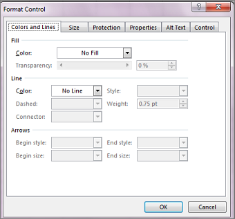
To choose a background color for your checkbox – right-click over the checkbox and click on the option «Format Control». Inside the «Format Control» window > «Color and Lines» tab > «Fill» section, you can choose a background color and desired transparency for your checkbox.
 30")
Selecting Border Color for the Checkbox Control
To create a checkbox border – Inside the «Format Control» window > «Color and Lines» tab > «Lines» section you can choose a border for your checkbox.
Choosing a 3D Shade Effect for Checkbox Control
To give your checkboxes a slight 3D effect – Inside the «Format Control» window > «Control» tab > 3-D shading option.
 31")
ActiveX Checkboxes In Excel
Until now, in this article, we have only talked about Excel Form Checkbox, but there is another type of checkbox that Microsoft Excel makes available – that is known as ActiveX Checkbox.
 32")
ActiveX checkboxes can also be added from the «Developer» Tab > «Insert» button. Also, in most aspects, an ActiveX checkbox is very similar to a form checkbox, but there are some critical differences between the two:
- ActiveX checkboxes provide more formatting options. In ActiveX checkboxes, you can change the checkbox caption font, have an image as a background, change the mouse pointer while it hovers over the checkbox, etc.
- ActiveX controls are external components and hence are loaded separately this sometimes causes them to freeze or become unresponsive. On the other hand, Form controls are built into Excel, and therefore they do not have any such issues.
- ActiveX is a Microsoft-based technology and is not supported by other operating systems like Mac.
- Also, many computers don’t trust ActiveX by default, and ActiveX controls are disabled unless you add them to the Trust Center.
- Another essential difference between the Form controls and ActiveX controls is that – ActiveX controls can be directly accessed as objects in the VBA Code (faster) whereas to access form controls you need to find the form controls on the active sheet (slower).
How to Assign a Macro to a Checkbox
We have already seen how to associate cell links with checkboxes in excel and perform actions based on the checkbox value. Now, let’s understand how to assign macros with checkboxes and execute the macros when the checkbox is clicked.
To associate a macro with the checkbox, follow these steps:
- Right-click over the checkbox and click the option «Assign Macro»
 33")
- On the «Assign Macro» window, give a meaningful name to the macro and click the «New» button, this will open the VBA editor.
 34")
- On the VBA editor, you can write the macro. For the sake of this example, we will be writing a macro that toggles the visibility of A Column. If the column is visible clicking the checkbox will hide it else if the column is hidden clicking the checkbox will unhide it.
 35")
- The VBA code is as follows:
Sub ToggleAColumnVisibility()
If ActiveSheet.Columns("A").Hidden = True Then
 Columns("A").Hidden = False
Else
 Columns("A").Hidden = True
End If
End Sub
- Save the macro and close the VBA editor.
 36")
- Now, try clicking on the checkbox and see how to toggles the visibility Column A.
Another example of using macro with excel checkbox: Selecting All Checkboxes using a Single Checkbox in Excel
Practical Examples of Using Checkboxes in Excel
Now let’s see some of the practical examples of excel checkboxes:
Example 1: Using Excel Checkboxes to Track Stock Availability for a Store
 37")
In the above example, we have a list of grocery items, with a checkbox against each one of them. The checkbox indicates the availability status of the item. As soon as the item is checked a label «Available» gets populated in-front of it and for unchecked checkboxes, a title «Out of Stock» is shown.
This is done simply by using built-in checkbox functionality and if statements. To accomplish this first, we have inserted a checkbox in the sheet and then selected its ‘cell link’ as the corresponding cell in range «E:E».
For instance, the ‘Cell link’ for checkbox at «B3» cell is «$E$3». And similarly, the ‘Cell link’ for checkbox at «B9» is «$E$9». This means – when the «B3» checkbox is checked the value at the «E3» cell will change to «True» otherwise the value will be «False».
 38")
Secondly, we have used an if based formula in front of these cells. The formula is:
=IF(E2=TRUE,"Available","Out of Stock")
The job of this IF statement is simply to read the value of the corresponding cell in «E:E» range and if its value is «True» then it displays a message «Available» otherwise the message will be «Out of Stock».
For instance, if the checkbox at ‘B6’ is checked so the value at ‘E6’ will be «True» and hence the value at ‘C6’ will be «Available».
Later, we have used an Excel Countif Function to find the total number of available items.
=COUNTIF(C2:C11,"Available")
And a similar COUNTIF Function is used for finding the total number of items unavailable:
=COUNTIF(C2:C11, "Out of Stock")
Example 2: Using Excel Checkboxes to create a To-Do List
 39")
In this example, we have a to-do list with tasks and their corresponding statuses represented by checkboxes. For each checkbox, the related cell link is set in the D-column in front of the checkbox.
Finally, in the summary section, we have counted the total number of tasks using the formula:
=COUNTA(D3:D13)
For calculating the completed tasks we have made use of the cell links, all the cell links with a value TRUE are considered to be associated with completed tasks. And based on this we have come up with a formula:
=COUNTIF($D$3:$D$13,TRUE)
 40")
Completed task percentage is calculated by using a simple percentage formula, i.e. (number of completed tasks/number of total tasks)*100 :
=B19/B18%
So, this was all about inserting and using a checkbox in Excel. Please feel free to share any comments or queries related to the topic.
На чтение 6 мин Опубликовано 07.01.2021
В Microsoft Office Excel в любую ячейку таблицы можно поставить чекбокс. Это специфический символ в виде галочки, предназначенный для оформления какой-либо части текста, выделения важных элементов, запуска сценариев. В данной статье будут рассмотрены методы установки знака в Эксель с помощью встроенных в программу инструментов.
Содержание
- Как установить флажок
- Способ 1. Использование стандартных символов Microsoft Excel
- Способ 2. Замена символов
- Способ 3. Постановка галочки для активации чекбокса
- Способ 4. Как создать чекбокс для реализации сценариев
- Способ 5. Установка чекбокса с использованием инструментов ActiveX
- Заключение
Как установить флажок
Поставить флажок в Excel достаточно просто. С этим значком презентабельность и эстетичность документа повысится. Подробнее о нем будет рассказано далее.
Способ 1. Использование стандартных символов Microsoft Excel
В Экселе, как и в Word, есть собственная библиотека различных символов, которые можно установить в любом месте рабочего листа. Чтобы найти значок галочки и разместить его в ячейке, необходимо выполнить следующие действия:
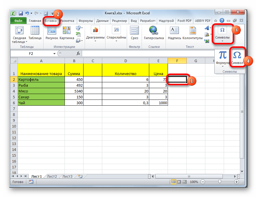
- Выделить ячейку, в которую надо поставить чекбокс.
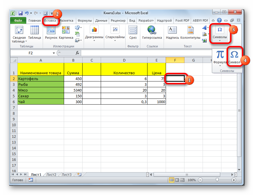
- Переместиться в раздел «Вставка» сверху главного меню.
- Нажать на кнопку «Символы» в конце списка инструментов.
- В открывшемся окне еще раз кликнуть по варианту «Символ». Откроется меню встроенных в программу значков.
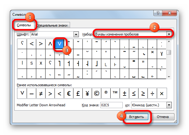
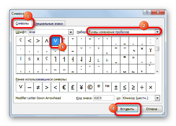
- В поле «Набор» указать вариант «Буквы изменения пробелов», найти знак галочки в представленном списке параметров, выделить его ЛКМ и щелкнуть по слову «Вставить» внизу окошка.
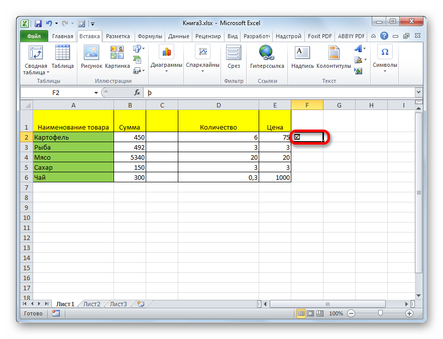
- Убедиться, что чекбокс вставился в нужную ячейку.
Обратите внимание! В каталоге символов есть несколько типов чекбоксов. Значок выбирается на усмотрение пользователя.
Способ 2. Замена символов
Выполнять вышеуказанные действия необязательно. Символ чекбокса можно прописать вручную с клавиатуры компьютера, переключив ее раскладку на английский режим и нажав на кнопку «V».
Способ 3. Постановка галочки для активации чекбокса
С помощью постановки или снятия флажка в Excel можно запускать различные сценарии. Для начала потребуется разместить чекбокс на рабочем листе, активировав режим разработчика. Для вставки данного элемента необходимо проделать следующие манипуляции:
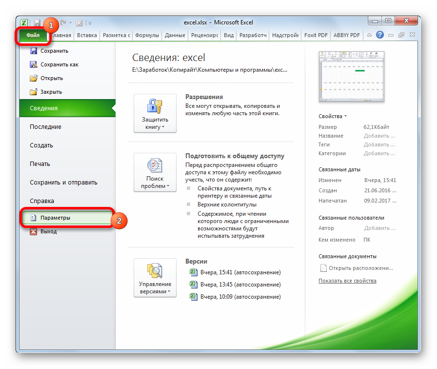
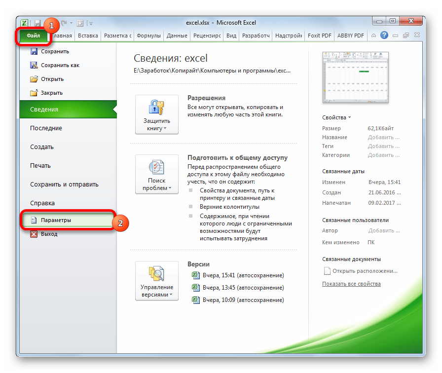
- Нажать по слову «Файл» в левом верхнем углу экрана.
- Перейти в раздел «Параметры».
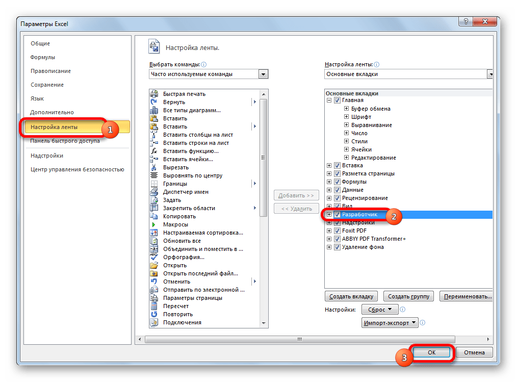
- В следующем окне надо выделить подраздел «Настройка ленты» в левой части экрана.
- В графе «Основные вкладки» в списке найти строку «Разработчик» и поставить галочку напротив этого параметра, после чего щелкнуть по «ОК» для закрытия окошка.
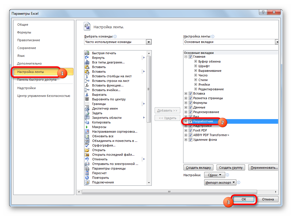
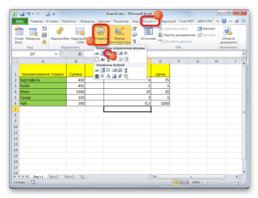
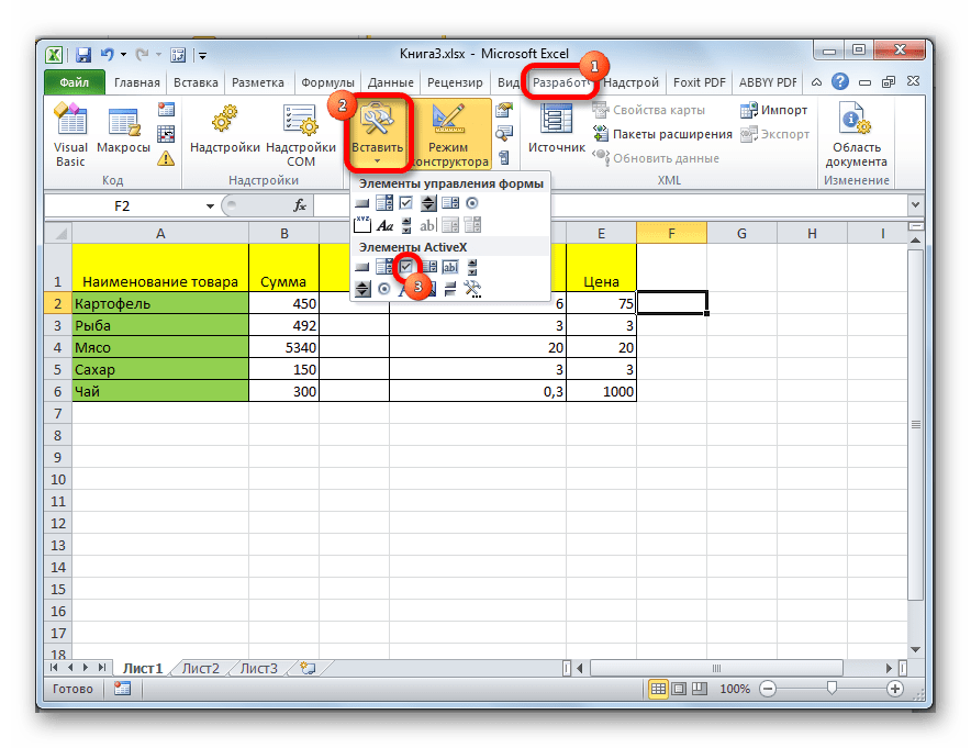
- Теперь в списке инструментов сверху главного меню программы появится вкладка «Разработчик». В нее нужно перейти.
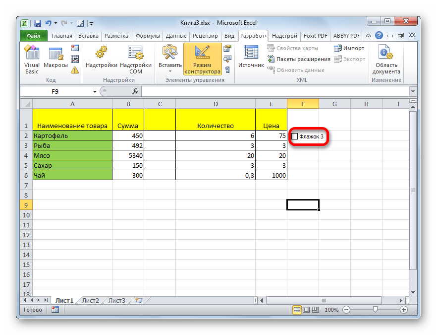
- В рабочем блоке инструмента кликнуть по кнопке «Вставить» и в графе «Элементы управления» формы щелкнуть по иконке чекбокса.
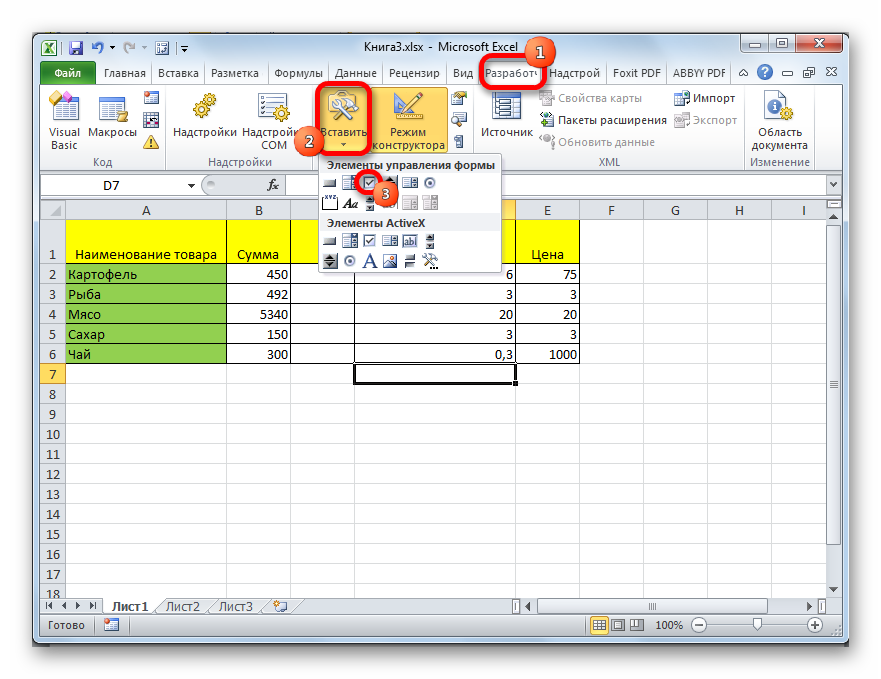
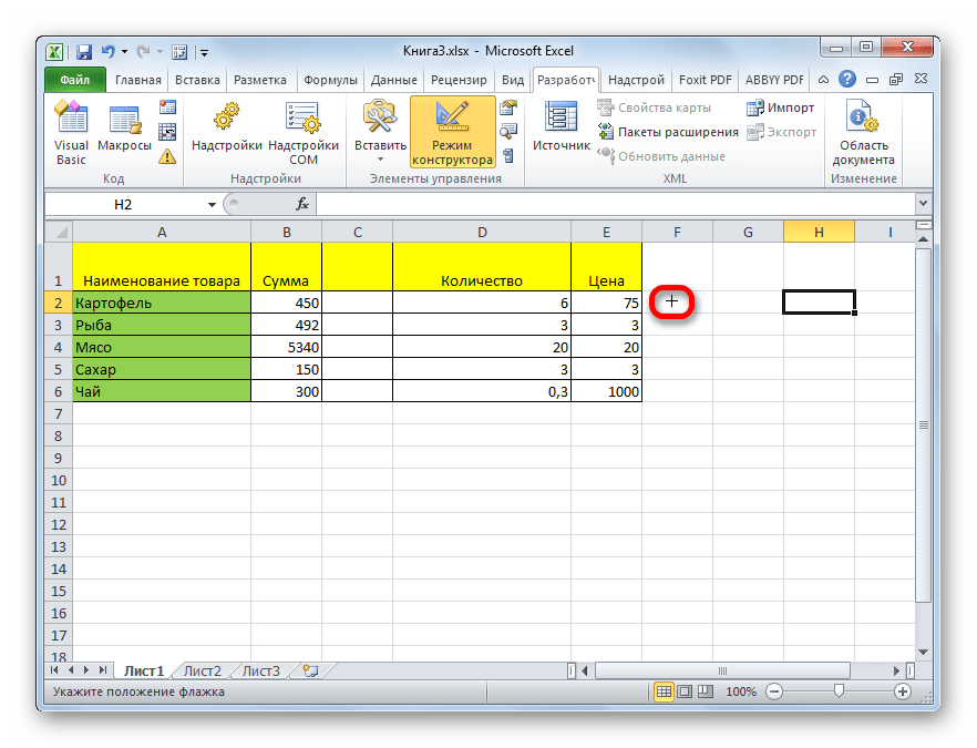
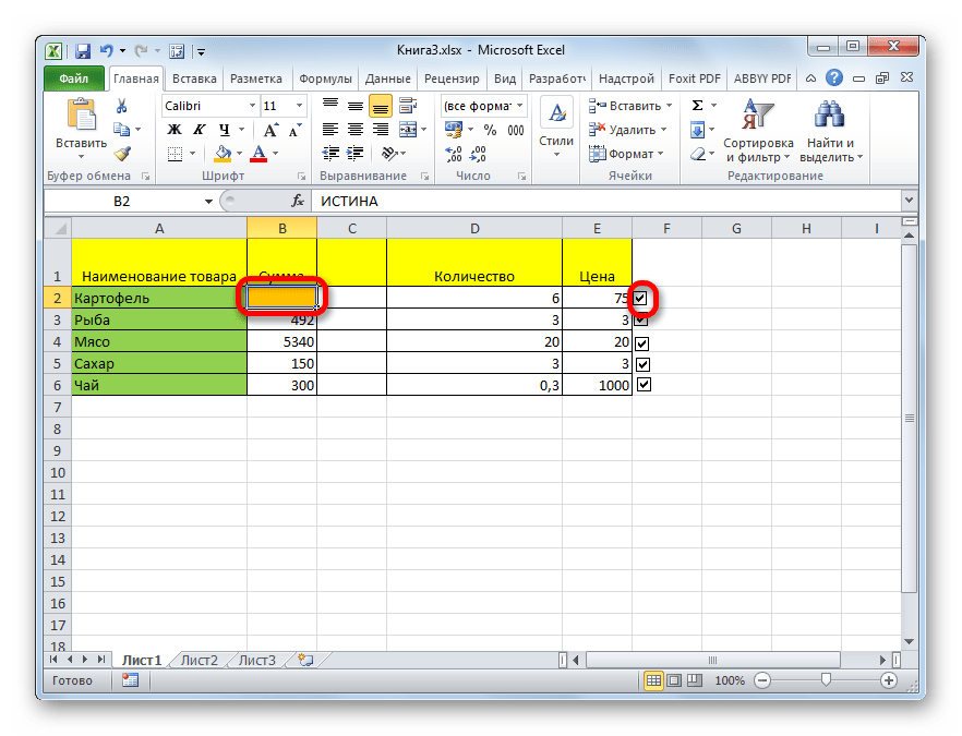
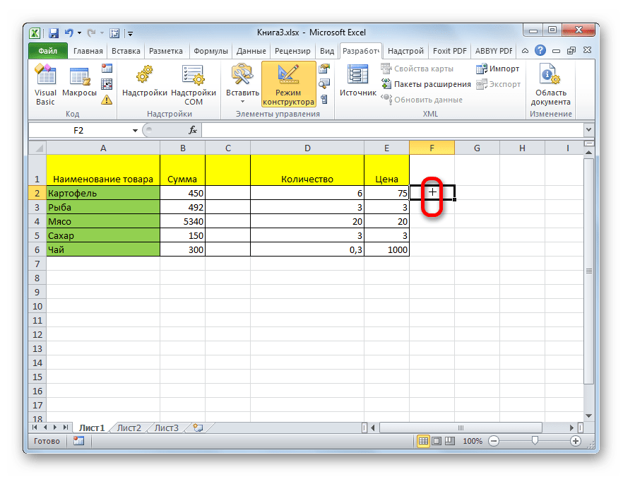
- После выполнения предыдущих действия вместо стандартного курсора мышки будет отображаться значок в виде крестика. На этом этапе пользователю надо кликнуть ЛКМ по области, в которую будет вставлена форма.
- Убедиться, что после клика в ячейке появился пустой квадратик.
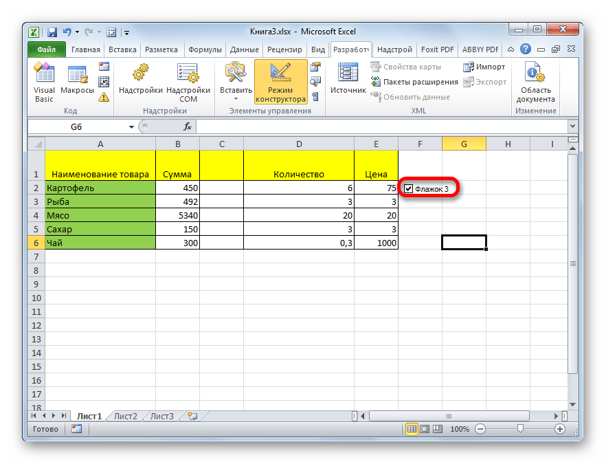
- Щелкнуть ЛКМ по этому квадратику, и в нем разместится флажок.
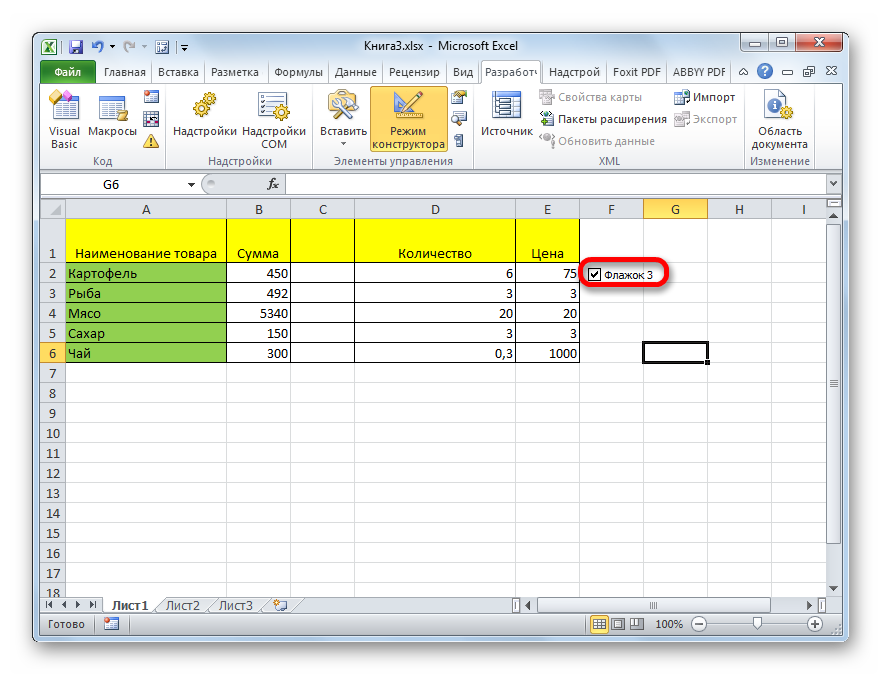
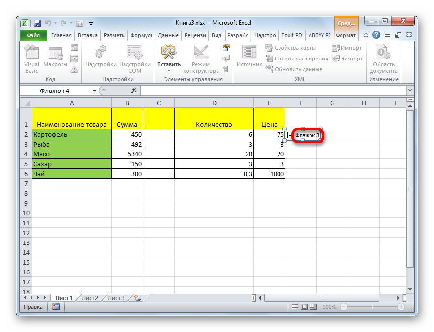
- Рядом с чекбоксом в ячейке будет находиться стандартная надпись. Ее потребуется выделить и нажать на клавишу «Delete» с клавиатуры, чтобы удалить.
Важно! Стандартную надпись, расположенную рядом со вставленным символом, можно заменить на любую другую на усмотрение пользователя.
Способ 4. Как создать чекбокс для реализации сценариев
Установленный в ячейке флажок можно использовать для выполнения того или иного действия. Т.е. на рабочем листе, в таблице будут вноситься изменения после установки или снятия галочки в квадратике. Чтобы реализовать такую возможность, необходимо:
- Выполнить действия, рассмотренные в предыдущем разделе, чтобы пометить значок в ячейке.
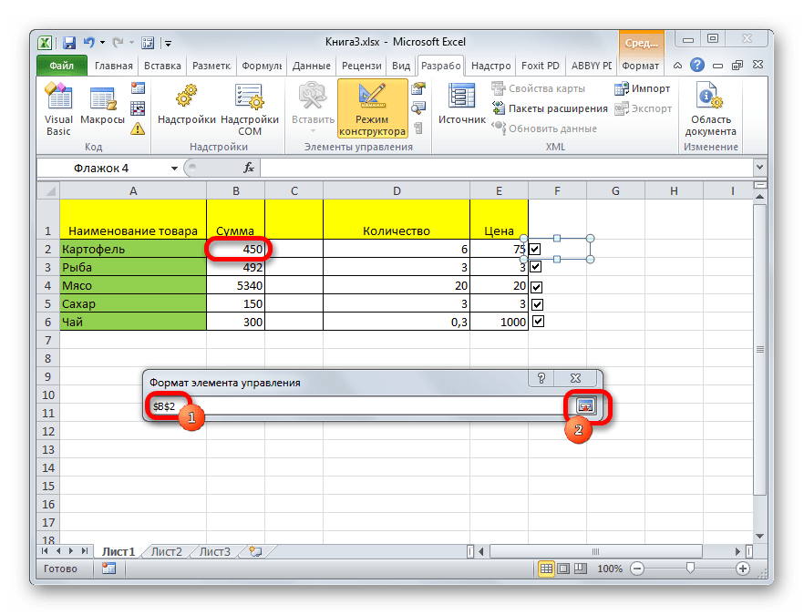
- Щелкнуть ЛКМ по вставленному элементу и перейти в меню «Формат объекта».
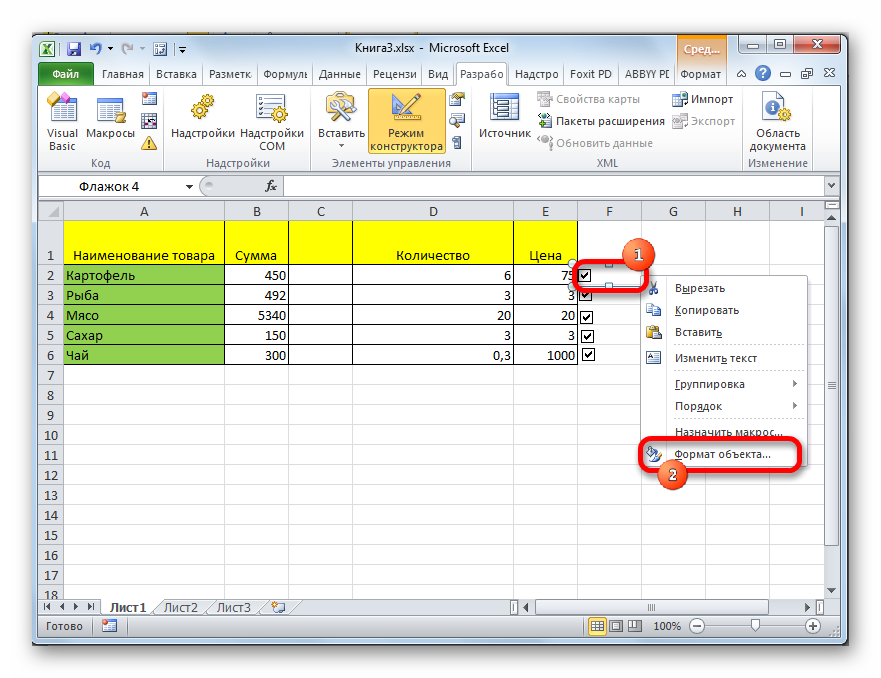
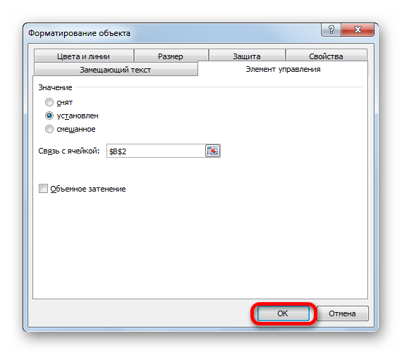
- Во вкладке «Элемент управления» в графе «Значение» поставить тумблер напротив строки, характеризующей текущее состояние чекбокса. Т.е. либо в поле «Установлен», либо в строчку «Снят».
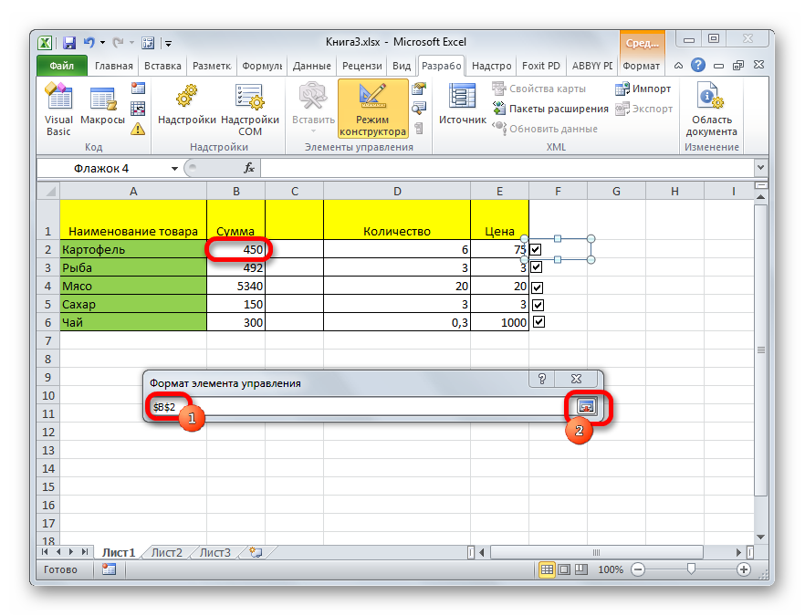
- Нажать на кнопку «Связать с ячейкой» внизу окна.
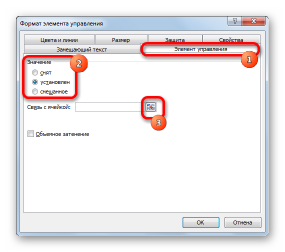
- Указать ячейку, в которой пользователь планирует запускать сценарии с помощью переключения чекбокса и еще раз кликнуть по тому же значку.
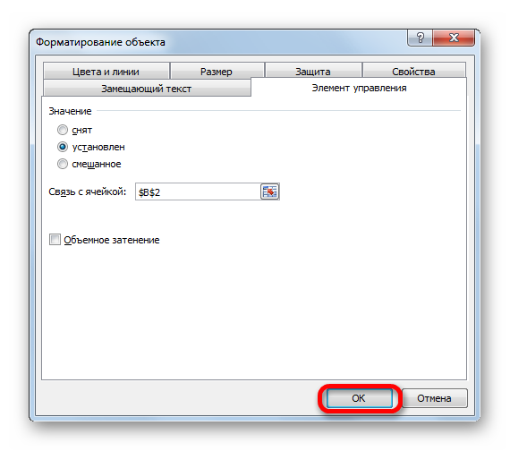
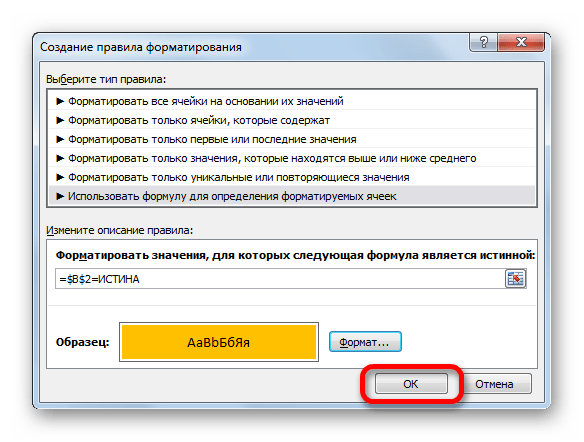
- В меню «Форматирование объекта» щелкнуть по «ОК», чтобы внесенные изменения применились.
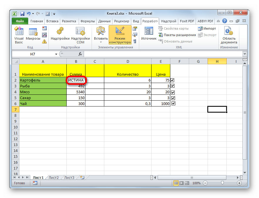
- Теперь после установки галочки в выбранной ячейки будет прописано слово «ИСТИНА», а после снятия значение «ЛОЖЬ».
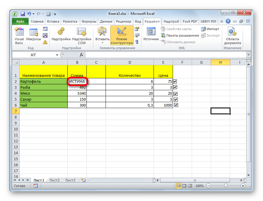
- К данной ячейке можно привязать любое действие, к примеру смену цвета.
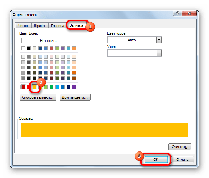
Дополнительная информация! Привязка цвета производится в меню «Формат ячеек» во вкладке «Заливка».
Способ 5. Установка чекбокса с использованием инструментов ActiveX
Такой метод можно будет реализовать после активации режима разработчика. В общем виде алгоритм выполнения задачи можно сократить следующим образом:
- Активировать режим разработчика по рассмотренной выше схеме. Подробная инструкция была приведена при рассмотрении третьего способа вставки флажка. Повторяться нецелесообразно.
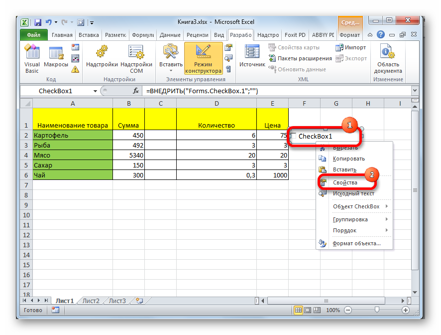
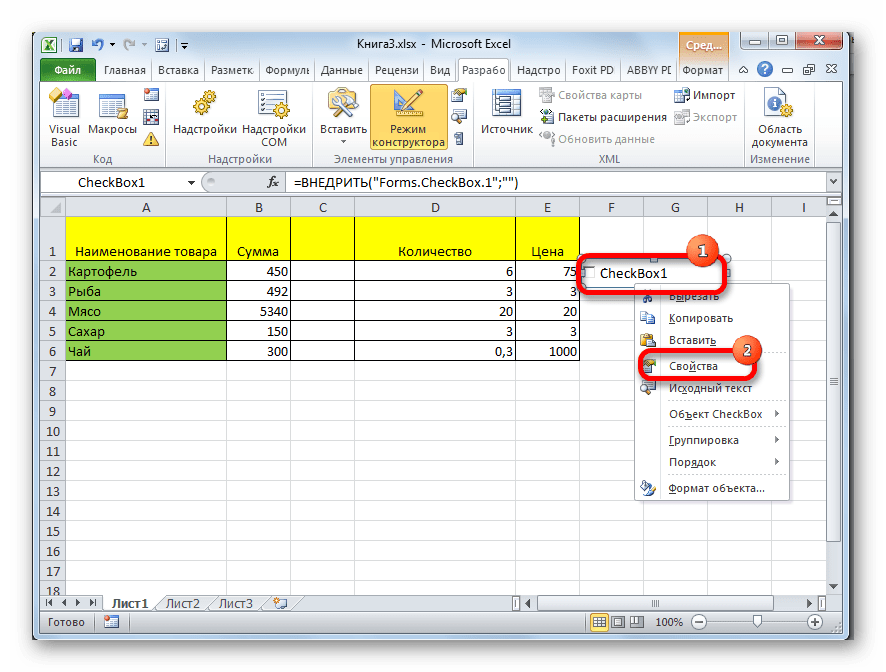
- Кликнуть правой клавишей манипулятора по ячейке с пустым квадратиком и стандартной надписью, которая появится после входа в режим «Разработчик».
- В контекстном меню выбрать пункт «Свойства».
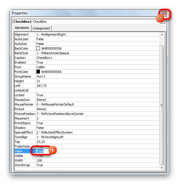
- Откроется новое окно, в списке параметров которого надо будет отыскать строку «Value» и вручную прописать слово «True» вместо «False».
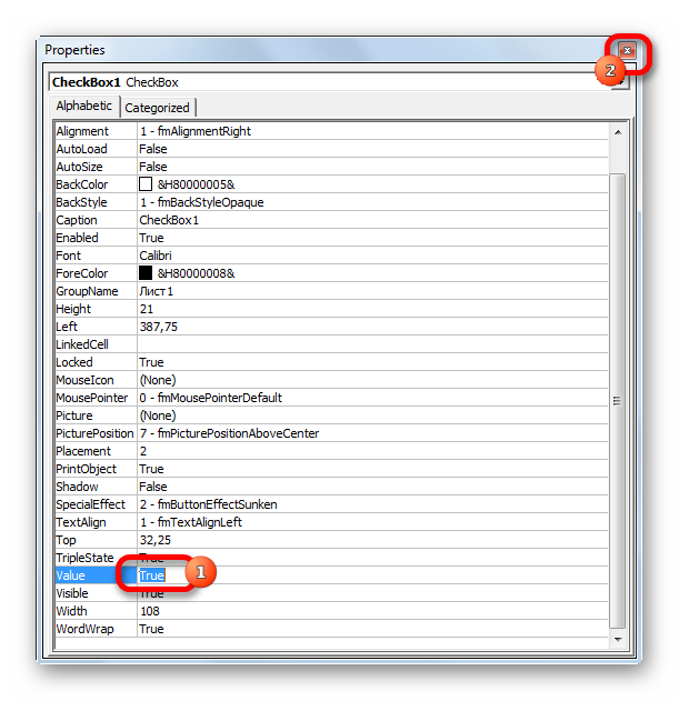
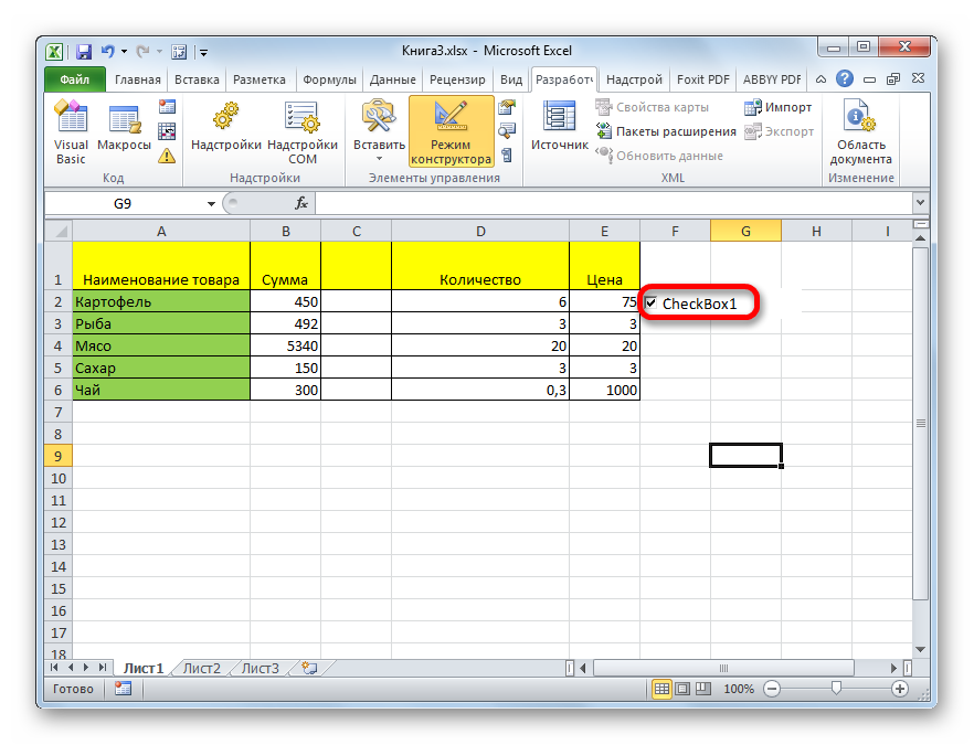
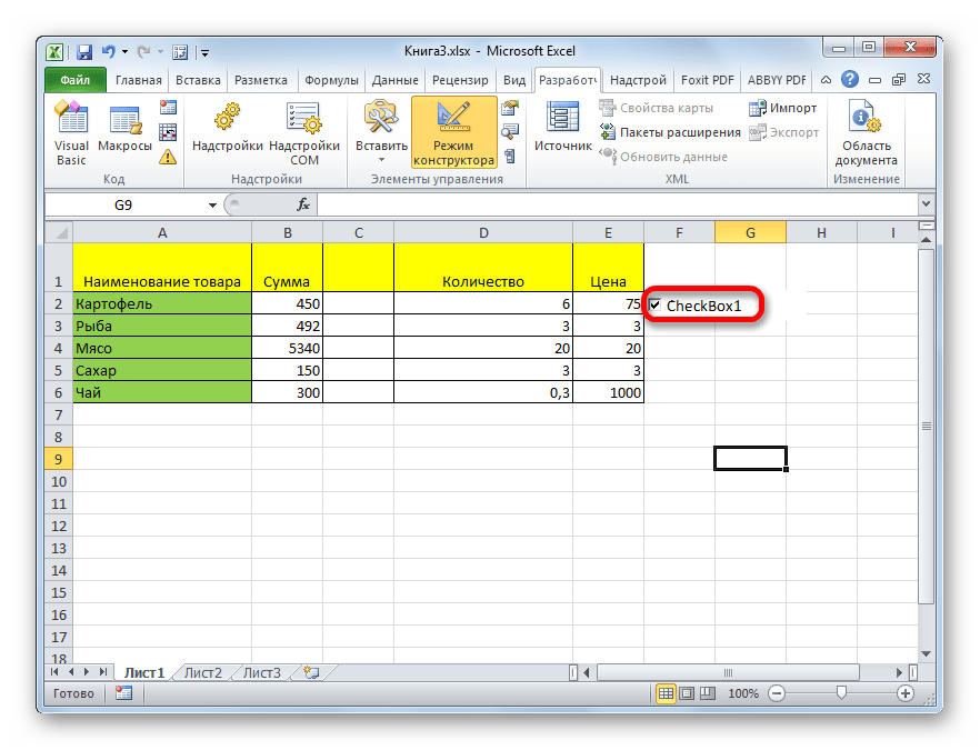
- Закрыть окно и проверить результат. Галочка должна появится в квадратике.
Заключение
Таким образом, в Excel чекбокс можно поставить различными способами. Выбор метода установки зависит от целей, преследуемых пользователем. Чтобы просто пометить тот или иной объект в табличке, достаточно воспользоваться методом подмены символов.
Оцените качество статьи. Нам важно ваше мнение:
Содержание
- Установка флажка
- Способ 1: вставка через меню «Символ»
- Способ 2: подмена символов
- Способ 3: установка галочки в чекбоксе
- Способ 4: создание чекбокса для выполнения сценария
- Способ 5: установка галочки с помощью инструментов ActiveX
- Вопросы и ответы

В программе Microsoft Office пользователю иногда нужно вставить галочку или, как по-другому называют этот элемент, флажок (˅). Это может быть выполнено для различных целей: просто для пометки какого-то объекта, для включения различных сценариев и т.д. Давайте выясним, как установить галочку в Экселе.
Установка флажка
Существует несколько способов поставить галочку в Excel. Для того чтобы определиться с конкретным вариантом нужно сразу установить, для чего вам нужна установка флажка: просто для пометки или для организации определенных процессов и сценариев?
Урок: Как поставить галочку в Microsoft Word
Способ 1: вставка через меню «Символ»
Если вам нужно установить галочку только в визуальных целях, чтобы пометить какой-то объект, то можно просто воспользоваться кнопкой «Символ» расположенной на ленте.
- Устанавливаем курсор в ячейку, в которой должна располагаться галочка. Переходим во вкладку «Вставка». Жмем по кнопке «Символ», которая располагается в блоке инструментов «Символы».
- Открывается окно с огромным перечнем различных элементов. Никуда не переходим, а остаемся во вкладке «Символы». В поле «Шрифт» может быть указан любой из стандартных шрифтов: Arial, Verdana, Times New Roman и т.п. Для быстрого поиска нужного символа в поле «Набор» устанавливаем параметр «Буквы изменения пробелов». Ищем символ «˅». Выделяем его и жмем на кнопку «Вставить».
После этого выбранный элемент появится в предварительно указанной ячейке.

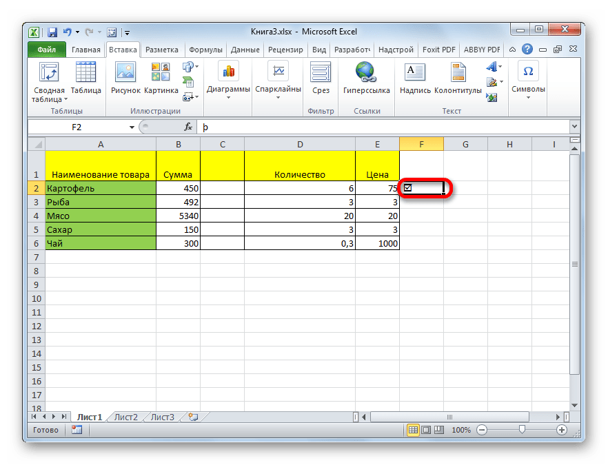
Таким же образом можно вставить более привычную нам галочку с непропорциональными сторонами или галочку в чексбоксе (небольшой квадратик, специально предназначенный для установки флажка). Но для этого, нужно в поле «Шрифт» указать вместо стандартного варианта специальный символьный шрифт Wingdings. Затем следует опуститься в самый низ перечня знаков и выбрать нужный символ. После этого жмем на кнопку «Вставить».
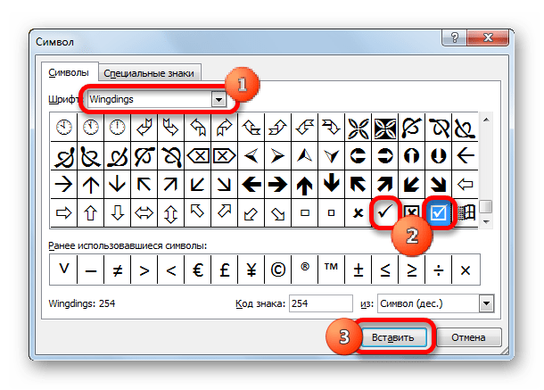
Выбранный знак вставлен в ячейку.
Способ 2: подмена символов
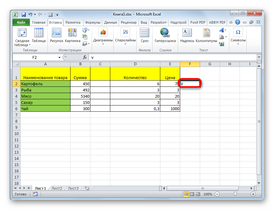
Есть также пользователи, которые не задаются точным соответствием символов. Поэтому вместо того, чтобы установить стандартную галочку, просто печатают с клавиатуры символ «v» в англоязычной раскладке. Иногда это оправдано, так как этот процесс занимает очень мало времени. А внешне эта подмена практически незаметна.

Способ 3: установка галочки в чекбоксе
Но для того, чтобы статус установки или снятия галочки запускал какие-то сценарии, нужно выполнить более сложную работу. Прежде всего, следует установить чекбокс. Это такой небольшой квадратик, куда ставится флажок. Чтобы вставить этот элемент, нужно включить меню разработчика, которое по умолчанию в Экселе выключено.
- Находясь во вкладке «Файл», кликаем по пункту «Параметры», который размещен в левой части текущего окна.
- Запускается окно параметров. Переходим в раздел «Настройка ленты». В правой части окна устанавливаем галочку (именно такую нам нужно будет установить на листе) напротив параметра «Разработчик». В нижней части окна кликаем по кнопке «OK». После этого на ленте появится вкладка «Разработчик».
- Переходим в только что активированную вкладку «Разработчик». В блоке инструментов «Элементы управления» на ленте жмем на кнопку «Вставить». В открывшемся списке в группе «Элементы управления формы» выбираем «Флажок».
- После этого курсор превращается в крестик. Кликаем им по той области на листе, где нужно вставить форму.

Появляется пустой чекбокс.
- Для установки в нем флажка нужно просто кликнуть по данному элементу и флажок будет установлен.
- Для того, чтобы убрать стандартную надпись, которая в большинстве случаев не нужна, кликаем левой кнопкой мыши по элементу, выделяем надпись и жмем на кнопку Delete. Вместо удаленной надписи можно вставить другую, а можно ничего не вставлять, оставив чекбокс без наименования. Это на усмотрение пользователя.
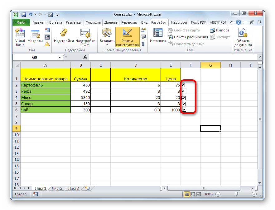
- Если есть потребность для создания нескольких чекбоксов, то можно не создавать для каждой строки отдельный, а скопировать уже готовый, что значительно сэкономит время. Для этого сразу выделяем форму кликом мыши, затем зажимаем левую кнопку и перетягиваем форму в нужную ячейку. Не бросая кнопку мыши, зажимаем клавишу Ctrl, а затем отпускаем кнопку мышки. Аналогичную операцию проделываем и с другими ячейками, в которые нужно вставить галочку.
Способ 4: создание чекбокса для выполнения сценария
Выше мы узнали, как поставить галочку в ячейку различными способами. Но данную возможность можно использовать не только для визуального отображения, но и для решения конкретных задач. Можно устанавливать различные варианты сценариев при переключении флажка в чекбоксе. Мы разберем, как это работает на примере смены цвета ячейки.
- Создаем чекбокс по алгоритму, описанному в предыдущем способе, с использованием вкладки разработчика.
- Кликаем по элементу правой кнопкой мыши. В контекстном меню выбираем пункт «Формат объекта…».
- Открывается окно форматирования. Переходим во вкладку «Элемент управления», если оно было открыто в другом месте. В блоке параметров «Значения» должно быть указано текущее состояние. То есть, если галочка на данный момент установлена, то переключатель должен стоять в позиции «Установлен», если нет – в позиции «Снят». Позицию «Смешанное» выставлять не рекомендуется. После этого жмем на пиктограмму около поля «Связь с ячейкой».
- Окно форматирования сворачивается, а нам нужно выделить ячейку на листе, с которой будет связан чекбокс с галочкой. После того, как выбор произведен, повторно жмем на ту же кнопку в виде пиктограммы, о которой шла речь выше, чтобы вернутся в окно форматирования.
- В окне форматирования жмем на кнопку «OK» для того, чтобы сохранить изменения.

Как видим, после выполнения данных действий в связанной ячейке при установленной галочке в чекбоксе отображается значение «ИСТИНА». Если галочку убрать, то будет отображаться значение «ЛОЖЬ». Чтобы выполнить нашу задачу, а именно произвести смену цветов заливки, нужно будет связать эти значения в ячейке с конкретным действием.
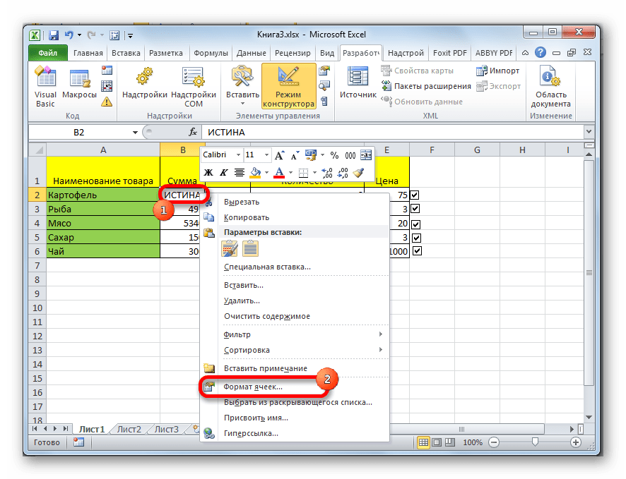
- Выделяем связанную ячейку и кликаем по ней правой кнопкой мыши, в открывшемся меню выбираем пункт «Формат ячеек…».
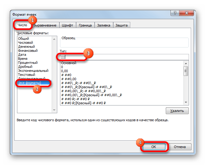
- Открывается окно форматирования ячейки. Во вкладке «Число» выделяем пункт «Все форматы» в блоке параметров «Числовые форматы». Поле «Тип», которое расположено в центральной части окна, прописываем следующее выражение без кавычек: «;;;». Жмем на кнопку «OK» в нижней части окна. После этих действий видимая надпись «ИСТИНА» из ячейки исчезла, но значение осталось.
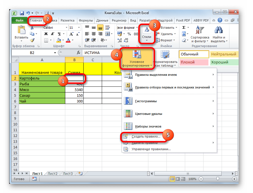
- Снова выделяем связанную ячейку и переходим во вкладку «Главная». Жмем на кнопку «Условное форматирование», которая размещена в блоке инструментов «Стили». В появившемся списке кликаем по пункту «Создать правило…».
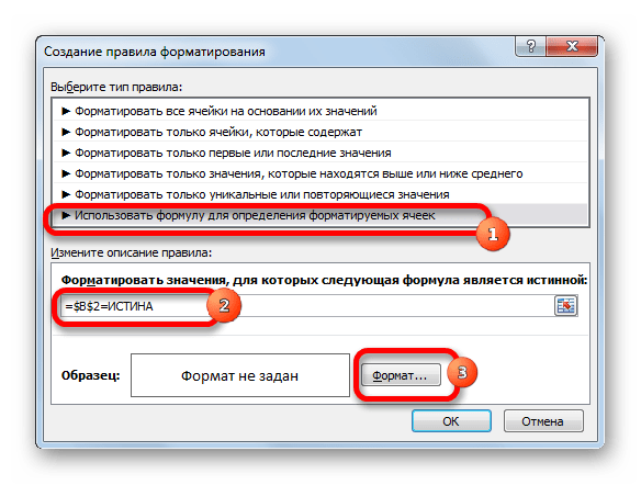
- Открывается окно создания правила форматирования. В его верхней части нужно выбрать тип правила. Выбираем самый последний в списке пункт: «Использовать формулу для определения форматируемых ячеек». В поле «Форматировать значения, для которых следующая формула является истиной» указываем адрес связанной ячейки (это можно сделать как вручную, так и просто выделив её), а после того, как координаты появились в строке, дописываем в неё выражение «=ИСТИНА». Чтобы установить цвет выделения, жмем на кнопку «Формат…».
- Открывается окно форматирования ячеек. Выбираем цвет, которым хотели бы залить ячейку при включении галочки. Жмем на кнопку «OK».
- Вернувшись в окно создания правила, жмем на кнопку «OK».


Теперь при включенной галочке связанная ячейка будет окрашиваться в выбранный цвет.
Если галочка будет убрана, то ячейка снова станет белой.

Урок: Условное форматирование в Excel
Способ 5: установка галочки с помощью инструментов ActiveX
Галочку можно установить также при помощи инструментов ActiveX. Данная возможность доступна только через меню разработчика. Поэтому, если эта вкладка не включена, то следует её активировать, как было описано выше.
- Переходим во вкладку «Разработчик». Кликаем по кнопке «Вставить», которая размещена в группе инструментов «Элементы управления». В открывшемся окне в блоке «Элементы ActiveX» выбираем пункт «Флажок».
- Как и в предыдущий раз, курсор принимает особую форму. Кликаем им по тому месту листа, где должна размещаться форма.
- Для установки галочки в чекбоксе нужно войти в свойства данного объекта. Кликаем по нему правой кнопкой мыши и в открывшемся меню выбираем пункт «Свойства».
- В открывшемся окне свойств ищем параметр «Value». Он размещается в нижней части. Напротив него меняем значение с «False» на «True». Делаем это, просто вбивая символы с клавиатуры. После того, как задача выполнена, закрываем окно свойств, нажав на стандартную кнопку закрытия в виде белого крестика в красном квадрате в верхнем правом углу окна.
После выполнения этих действий галочка в чекбоксе будет установлена.
Выполнение сценариев с использованием элементов ActiveX возможно при помощи средств VBA, то есть, путем написания макросов. Конечно, это намного сложнее, чем использование инструментов условного форматирования. Изучение этого вопроса – отдельная большая тема. Писать макросы под конкретные задачи могут только пользователи со знанием программирования и обладающие навыками работы в Эксель гораздо выше среднего уровня.
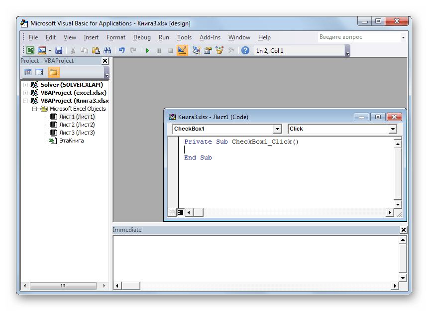
Для перехода к редактору VBA, с помощью которого можно будет записать макрос, нужно кликнуть по элементу, в нашем случае по чекбоксу, левой кнопкой мыши. После этого будет запущено окно редактора, в котором можно выполнять написание кода выполняемой задачи.
Урок: Как создать макрос в Excel
Как видим, существует несколько способов установить галочку в Экселе. Какой из способов выбрать, в первую очередь зависит от целей установки. Если вы хотите просто пометить какой-то объект, то нет смысла выполнять задачу через меню разработчика, так как это займет много времени. Намного проще использовать вставку символа или вообще просто набрать на клавиатуре английскую букву «v» вместо галочки. Если же вы хотите с помощью галочки организовать выполнение конкретных сценариев на листе, то в этом случае данная цель может быть достигнута только с помощью инструментов разработчика.
How to Insert a Checkbox in Excel: Easy Step-by-Step Guide (2023)
If you want to collect user input in your spreadsheet there’s no better way than the checkbox.

User-friendly, slick-looking, and easy for you to work with. Well… After you learn it at least.
If you’re having a hard time understanding the ins and outs of checkboxes, look no further.
Whether you’re into looks or functionality, I’ll guide you through everything step-by-step.
If you want to tag along, please download my sample data workbook here.
Let’s dive in🤿
Adding the Developer tab to Excel
There’s only one way to create a checkbox in Excel, and that’s from the Developer tab.
So, if you don’t see the Developer tab in your Ribbon already, you need to insert it first.
1. Click File on the Ribbon, and then click Options.
2. Click on ‘Customize Ribbon’.
3. Make sure there’s a checkmark in the Developer checkbox (kinda meta, right?)

Click OK and now the Developer tab is visible from the Excel Ribbon.
How to insert a checkbox in Excel
Here we have a small list of upsells.
In this list, a salesperson or the customer should be able to easily select the relevant upsells to the order.
And checkboxes are the perfect tools for that.
Eventually, we want that list to be able to calculate the total upsell price automatically, based on the selections. But, let’s save that for later and start with just getting the checkboxes into the spreadsheet.
1. Go to the Developer tab (here’s how to add it) and click Insert.
2. In the menu that appears, pick the Check Box form control.

Don’t select the ActiveX Check Box control. The reason why is complicated but for 99% of checkbox creators, the ‘Form Controls’ Checkbox is more than enough👍
3. Insert the checkbox by dragging its outline in your spreadsheet somewhere.

4. Change the name and size of the checkbox, and move it so it fits what you’re trying to achieve.
The checkbox doesn’t have to have a visible name. You can just double-click the name and delete it, and make the checkbox all small like this if you want.

Voila! Now the user (and you) can left-click the checkbox to put a checkmark in it🙌
Insert multiple checkboxes in Excel
Now, you’ve learned how to insert a checkbox in Excel.
Easy peasy lemon squeezy🍋
But in many cases, you want to insert multiple checkboxes.
You do that by first inserting one checkbox, and then copying either the checkbox or the cell that contains the checkbox.
1. After you’ve inserted a checkbox, right-click it and select ‘Format control’.

2. In the ‘Format Control’ dialog box go to the Properties tab.
3. Make sure the middle option ‘Move but don’t size with cells’ is selected and click OK.

4. Now, copy (or drag) the cell containing the original checkbox anywhere you want it.

Visually, the upsell list is complete👏
Users are now able to indicate which upsells they want.

BUT this doesn’t do anything but visually indicate the user’s choices.
By linking the checkboxes to cells we can make it calculate the upsells total automatically.
How to link checkboxes to cells
Now, this is where the fun begins.
A visual checkmark in a checkbox doesn’t allow for any calculation. It’s pure visuals.
But you can link the checkbox to a cell so it displays a TRUE or FALSE value when it’s checked or unchecked.
It’s basically like making a cell reference.
1. Right-click on the first checkbox and click ‘Format Control’

2. In the ‘Format Control’ dialog box, go to the ‘Control’ tab.
3. Select the ‘Unchecked’ option (radio button). That ensures the checkbox is unchecked by default when you open the spreadsheet containing it.
If you want the checkboxes to be checked by default, then select that option instead🕵️♂️

4. In the ‘Cell link’ box make a reference to the cell you wish to display either TRUE or FALSE depending if the checkbox is checked or unchecked.
Checked = TRUE, unchecked = FALSE.

5. Do the same for all the checkboxes.
It should look like this by now.

If the FALSE (or TRUE) values don’t show, try checking and unchecking the checkboxes a few times.
Now, all you need is a formula that adds up the upsells.
6. Write the formula:
=SUMIF(D2:D5, “TRUE”, B2:B5)

And that’s it!
Your interactive user interface now adds up the upsell prices from the chosen upsells. All selected by checking and unchecking cool-looking checkboxes.
Well done💪
To make this look prettier, change the font color to white on all the linked cells.
Conditional formatting based on checkboxes
Now that you have established a cell link from the checkbox to the cell, you can do lots of things with it.
You can even use conditional formatting to add some visual interactivity.
That could be something like highlighting the text if the checkbox is checked. This works quite well when you have multiple checkboxes.

Let’s try that.
1. If you haven’t already, insert cell links from your checkboxes.
2. Select the titles of the items, in A2:A5, and click ‘Conditional formatting’ on the Home tab.
3. Click on ‘New rule’ and select ‘Use a formula to select which cells to format’.
4. Type the formula: =D2=TRUE
5. Define the format you want to apply if the formula is true and press OK.
Now, the upsell names are highlighted when the checkbox is checked – all due to linked cells.

How to format your checkbox
If you want to make your checkbox look a little cooler, you can format it (almost) any way you want to.
Note that this formatting is static (normal formatting) and not dynamic (conditional formatting).
1. Right-click your checkbox and click ‘Format Control’.
2. In the control dialog box, go to the ‘Colors and Lines’ tab.

3. Choose the formatting you want and press OK.
And if you’re feeling crazy, you might end up with something like this🎉

VIDEO: How to insert checkboxes in Excel
Watch this video to learn how to insert a checkbox in Excel in just a few minutes.
That’s it – Now what?
That’s how to insert a checkbox in Excel.
Pretty cool, huh?😎
I hope you’re as excited about the interactive capabilities of checkboxes as I am.
As I described earlier, automation functions like IF and SUMIF, and even VLOOKUP, work great with checkboxes in Excel.
So, do you want to learn how to use these functions?
Then enroll in my free 3-part training and learn them (+ pivot tables) in 30 minutes.
Other resources
As I showed you in this guide, conditional functions such as IF/IFS and SUMIF work very well with a checkbox in Excel.
If you want to geek out on the possibilities in the developer tab, read more about it here.
Also, if you don’t need an actual checkbox but just the checkmark symbol, you can read up on that here.
Frequently Asked Questions
If I didn’t answer all your questions in the guide, please have a look below. Maybe you’re lucky🤞
The same method is used to delete multiple checkboxes but you must hold down Shift while right-clicking the checkboxes.
You insert the checkmark symbol by going to the Insert tab and clicking the Symbols button to the right.
Pick the check mark symbol and insert it in your spreadsheet.
Kasper Langmann2023-02-23T11:18:57+00:00
Page load link
Adding a checkbox to your workbook may sound simple but it can expand the possibilities of what you can do in Excel.

From checklists to graphs, there’s so much you can do. However, it starts with the checkbox.
Learn everything you need to know about checkboxes below.
![Download 10 Excel Templates for Marketers [Free Kit]](https://no-cache.hubspot.com/cta/default/53/9ff7a4fe-5293-496c-acca-566bc6e73f42.png)
-
Add the developer tab to your Ribbon.

-
Navigate to the Developer tab and locate the «Checkbox» option.
-
Select the cell where you want to add the checkbox control then click the checkbox.
-
Right-click the checkbox to edit the text and adjust sizing.
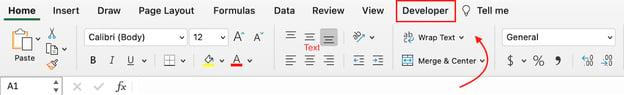
To do this on Windows, click File > Options > Customize Ribbon. Then, select the Developer checkbox and click «save.» On IOS, click Excel > Preferences > Ribbon & Toolbar > Main Tabs. Then, select the Developer checkbox and save.
On Windows, there are a few extra steps to see the checkbox option. Under the Developer tab, click «Insert» and under «Form Controls,» click the checkbox icon.
Note: Currently, you cannot use checkboxes in the web version of Excel. If you upload a workbook with these controls, you’ll first have to disable them to start editing.
How to Format a Checkbox in Excel
-
Open up the format control.
-
Modify the value and cell link, then click «OK.»
To access it on Windows, right-click the checkbox and select «Format Control.» On IOS, navigate to the «Format» tab and select «Format Control.»
With value, there are three options:
- Unchecked – This displays a box that is unchecked and returns a «FALSE» statement.
- Checked – This displays a box that is checked and returns a «TRUE» statement.
- Mixed – This will leave the checkbox empty as neither a true or false statement until an action is taken.
As for the cell link, this contains the checkbox status (true or false) of the cell it’s referencing.
Now that you have those details down, you can start fully customizing your checkbox.
How to Delete A Checkbox in Excel
Deleting a checkbox in Excel is a simple two-step process:
- Right-click the checkbox.
- Click «delete» on your keyboard.

One of the most demanding and fascinating things for an Excel user is to create interactive things in Excel. And a checkbox is a small but powerful tool that you can use to control a lot of things by unchecking/checking it.
In short: It gives you the power to make your stuff interactive. And, I’m sure you use it in your work, frequently. But, the thing is: Do you know how to use a checkbox up to its best? Yes, that’s the question.
In today’s post, I’m going to show you exactly how you can insert a checkbox in Excel and all the other things which will help you to know about its properties and options. So without any further ado, let’s explore this thing.
Here you have two different methods to insert a checkbox. You can use any of these methods which you think are convenient for you.
Manual Method
- First of all, go to the developer tab and if you are unable to see the developer tab in your ribbon, you can use these simple steps to enable it.

- In the Developer Tab, go to Controls → Form Controls → Select Checkbox.
- After selecting the check box click on the place on your worksheet where you want to insert it.
VBA Code
This is another method to insert a checkbox, you can use the following VBA code.
ActiveSheet.CheckBoxes.Add(left, Right, Height, Width).Select
ActiveSheet.CheckBoxes.Add(80, 40, 72, 72).Select
Using the above method is only helpful when you exactly know the place to insert and the size of the checkbox. Learn more about this method here.
Link a Checkbox with a Cell
Once you insert a checkbox in your worksheet the next thing you need to do is to link it with a cell. Follow these simple steps.
- Right-click on the check box and select format control.

- Now, you’ll get a format control dialog box.
- Go to the control tab and in the cell link input bar enter the cell address of the cell which you want to link with the checkbox.
- Click OK.
- In the cell which you have linked with your checkbox, you’ll get TRUE when you tick the checkbox and FALSE when you un-tick.

Deleting a Checkbox
You can delete a checkbox using two ways. The first way is to select a checkbox and press delete. This is a simple and fast method to do that.
And if you have more than one checkbox in your worksheet. Select all the checkboxes by holding the control key and pressing delete to delete them all. The second way is to use the selection pane to delete them
- Go to Home Tab → Editing → Find & Select → Selection Pane.
- In the selection pane, you will get the list of all the checkboxes you have used in your worksheet.
- You can select each of them one by one or you can select more than one by using the control key.
- Once you select them, press delete.
Printing a Checkbox
Most of the time users avoid printing a checkbox. But if you want to do that you can enable this option by using the following way.
- Right-click on the checkbox, and select Format Control.
- Go to Properties Tab.
- Tick mark “Print Object”.

This will allow you to print check boxes, and if you don’t want to print them make sure to untick this option.
Resizing a Checkbox
If you want to resize the checkbox you can simply expand its size by using dots from its border. And, if you want to resize it using a particular height and& width, you can do it by using the following steps.
- Right-click on the checkbox and select the format control option.
- Go to Size -> Tab Size and Rotate.
- Enter the height and width that you want to fix for the checkbox.
- Click OK.

Quick Tip: To lock the aspect ratio for the size of the checkbox tick mark “Lock aspect ratio”.
Copy a Checkbox in Multiple Cells
You can use three different ways to copy a checkbox from one place to another.
Copy Paste
- Select a checkbox.
- Right-click on it and copy it.
- Go to the cell where you want to paste that checkbox.
- Right-click and paste.
Use Control Key
- Select a checkbox.
- Press the control key.
- Now with your mouse, drag that checkbox to another place where you want to paste it.
Using Fill Handle
- Select the cell on which you have your checkbox.
- Use the fill handle and drag it up to the cell on which you want to copy the checkbox.
Renaming a Checkbox
While renaming a checkbox, there is one thing you have to keep in mind you have two different names associated with a checkbox. Caption name and an actual name of a checkbox.
- Question: How to change the caption name of a checkbox?
- Answer: Right-click and select edit text and then delete the default text and enter new text.
- Question: How to rename a checkbox?
- Answer: Right-click on the check box. Go to the address bar and edit the name. Change to the name you want and press enter.
Fixing the Position of a Checkbox
By default when you insert a checkbox in excel it will change its position & shape when you expand the cell on which it is placed.
But you can easily fix its position using these steps.
- Right, click on the checkbox, and go to Format Control → Properties Tab.
- In object positioning, select “don’t move or size with cell”.
- Once you select this option, the checkbox will not move from its position by expanding the column or row.
Hide or Un-hide a Checkbox
You can also hide or un-hide a check box from your worksheet using these steps.
- Open the selection pane by using the shortcut key Alt + F10.
- On the right side of the name of every checkbox, there is a small icon of an eye.
- Click on that icon to hide a checkbox and the same icon again to unhide it.
- If you want to hide/unhide all the checks boxes you can use the hide all button and show all buttons to show all the checkboxes.
How to use Checkbox in Excel
Here I have a list of useful ideas to use as a checkbox in your spreadsheet.
Creating a Checklist
In the below example, I have used a checkbox to create a checklist. And, I have used formulas in conditional formatting to create this checklist.
- Insert a check box and link it to a cell.
- Now, select the cell in which you have the task name and go to Home Tab -> Styles -> Conditional Formatting -> New Rule.
- Click on “Use a formula to determine which cell to format” and enter the below formula into it.
- =IF(B1=TRUE,TRUE,FALSE)
- Apply formatting for strikethrough.
- Click OK.
Now, whenever you tick the checkbox it will change the value in the linked cell to TRUE, and the cell in which you have applied conditional formatting will get a line through a value.
Create a Dynamic Chart with a Checkbox
In the below example, I have created a dynamic chart using a line chart and a column chart.
- Create a table with profit values and link it to another table using the below formula.
- =IF($I$17=TRUE,VLOOKUP($I4,$M$3:$N$15,2,0),NA())
- Then linked $I$17 with the checkbox.
- Whenever I tick that checkbox, the above formula will use VLOOKUP Function to get profit percentages. And, if a checkbox is unticked I’ll get a #N/A.
Use Checkbox to Run a Macro
While working on an invoice template I got this idea. The idea is if you want to insert the shipping address the same as the billing address you just have to tick the checkbox and the address will be copied to it.
And, on the other side when you untick that checkbox content will be cleared.
- Go to the Developer Tab → Code → Visual Basic or you can also use the shortcut key to open the visual basic editor.
- Add below VBA code to the sheet in which you have inserted your checkbox.
Sub Ship_To_XL()

If Range(“D15”) = True Then
Range("D17:D21") = Range("C17:C21")

Else
If Range(“D15”) = False Then
Range("D17:D21").ClearContents

Else: MsgBox (“Error!”)

End If

End Sub
Please note you have to insert this code into the code window of the same worksheet in which you want to use it. In the above code, D17:D21 is the range for the shipping address and C17:C21 is the range for the billing address. In cell D15, I have linked the checkbox.
sample-file