
If you find yourself needing to expand or reduce Excel’s row widths and column heights, there are several ways to adjust them. The table below shows the minimum, maximum and default sizes for each based on a point scale.
|
Type |
Min |
Max |
Default |
|---|---|---|---|
|
Column |
0 (hidden) |
255 |
8.43 |
|
Row |
0 (hidden) |
409 |
15.00 |
Notes:
-
If you are working in Page Layout view (View tab, Workbook Views group, Page Layout button), you can specify a column width or row height in inches, centimeters and millimeters. The measurement unit is in inches by default. Go to File > Options > Advanced > Display > select an option from the Ruler Units list. If you switch to Normal view, then column widths and row heights will be displayed in points.
-
Individual rows and columns can only have one setting. For example, a single column can have a 25 point width, but it can’t be 25 points wide for one row, and 10 points for another.

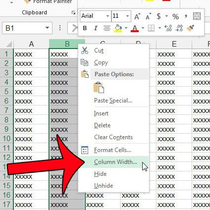
Set a column to a specific width
-
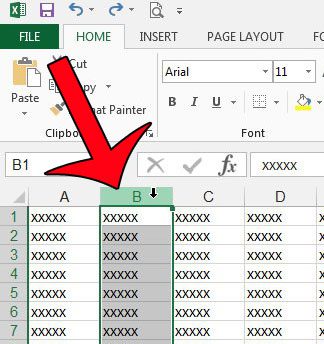
Select the column or columns that you want to change.
-
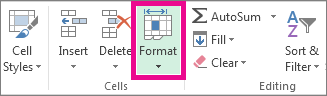
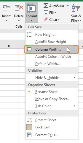
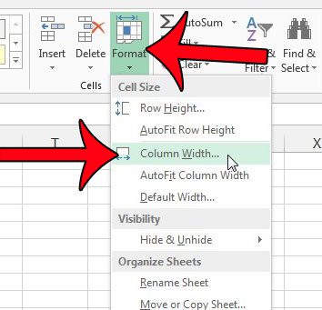
On the Home tab, in the Cells group, click Format.

-
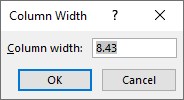
Under Cell Size, click Column Width.
-
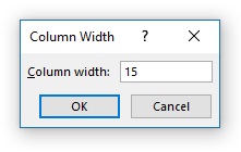
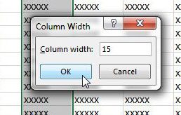
In the Column width box, type the value that you want.
-
Click OK.
Tip: To quickly set the width of a single column, right-click the selected column, click Column Width, type the value that you want, and then click OK.
-
Select the column or columns that you want to change.
-
On the Home tab, in the Cells group, click Format.
-
Under Cell Size, click AutoFit Column Width.
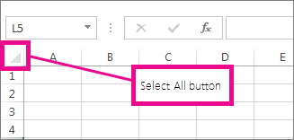
Note: To quickly autofit all columns on the worksheet, click the Select All button, and then double-click any boundary between two column headings.
-
Select a cell in the column that has the width that you want to use.
-
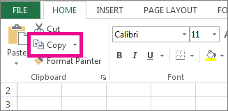
Press Ctrl+C, or on the Home tab, in the Clipboard group, click Copy.
-
Right-click a cell in the target column, point to Paste Special, and then click the Keep Source Columns Widths
button.
 button.
The value for the default column width indicates the average number of characters of the standard font that fit in a cell. You can specify a different number for the default column width for a worksheet or workbook.
-
Do one of the following:
-
To change the default column width for a worksheet, click its sheet tab.
-
To change the default column width for the entire workbook, right-click a sheet tab, and then click Select All Sheets on the shortcut menu.
-
-
On the Home tab, in the Cells group, click Format.
-
Under Cell Size, click Default Width.
-
In the Standard column width box, type a new measurement, and then click OK.

Do one of the following:
-
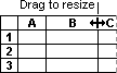
To change the width of one column, drag the boundary on the right side of the column heading until the column is the width that you want.
-
To change the width of multiple columns, select the columns that you want to change, and then drag a boundary to the right of a selected column heading.
-
To change the width of columns to fit the contents, select the column or columns that you want to change, and then double-click the boundary to the right of a selected column heading.
-
To change the width of all columns on the worksheet, click the Select All button, and then drag the boundary of any column heading.
-
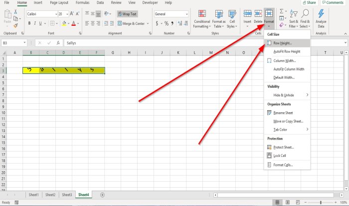
Select the row or rows that you want to change.
-
On the Home tab, in the Cells group, click Format.
-
Under Cell Size, click Row Height.
-
In the Row height box, type the value that you want, and then click OK.
-
Select the row or rows that you want to change.
-
On the Home tab, in the Cells group, click Format.
-
Under Cell Size, click AutoFit Row Height.
Tip: To quickly autofit all rows on the worksheet, click the Select All button, and then double-click the boundary below one of the row headings.
Do one of the following:
-
To change the row height of one row, drag the boundary below the row heading until the row is the height that you want.
-
To change the row height of multiple rows, select the rows that you want to change, and then drag the boundary below one of the selected row headings.
-
To change the row height for all rows on the worksheet, click the Select All button, and then drag the boundary below any row heading.
-
To change the row height to fit the contents, double-click the boundary below the row heading.

Top of Page
If you prefer to work with column widths and row heights in inches, you should work in Page Layout view (View tab, Workbook Views group, Page Layout button). In Page Layout view, you can specify a column width or row height in inches. In this view, inches are the measurement unit by default, but you can change the measurement unit to centimeters or millimeters.
-
In Excel 2007, click the Microsoft Office Button
> Excel Options> Advanced. -
In Excel 2010, go to File > Options > Advanced.
 > Excel Options> Advanced.
Set a column to a specific width
-
Select the column or columns that you want to change.
-
On the Home tab, in the Cells group, click Format.
-
Under Cell Size, click Column Width.
-
In the Column width box, type the value that you want.

-
Select the column or columns that you want to change.
-
On the Home tab, in the Cells group, click Format.
-
Under Cell Size, click AutoFit Column Width.
Tip To quickly autofit all columns on the worksheet, click the Select All button and then double-click any boundary between two column headings.

-
Select a cell in the column that has the width that you want to use.
-
On the Home tab, in the Clipboard group, click Copy, and then select the target column.
-
On the Home tab, in the Clipboard group, click the arrow below Paste, and then click Paste Special.
-
Under Paste, select Column widths.

The value for the default column width indicates the average number of characters of the standard font that fit in a cell. You can specify a different number for the default column width for a worksheet or workbook.
-
Do one of the following:
-
To change the default column width for a worksheet, click its sheet tab.
-
To change the default column width for the entire workbook, right-click a sheet tab, and then click Select All Sheets on the shortcut menu.
-
-
On the Home tab, in the Cells group, click Format.
-
Under Cell Size, click Default Width.
-
In the Default column width box, type a new measurement.

Tip If you want to define the default column width for all new workbooks and worksheets, you can create a workbook template or a worksheet template, and then base new workbooks or worksheets on those templates. For more information, see Save a workbook or worksheet as a template.
Do one of the following:
-
To change the width of one column, drag the boundary on the right side of the column heading until the column is the width that you want.
-
To change the width of multiple columns, select the columns that you want to change, and then drag a boundary to the right of a selected column heading.
-
To change the width of columns to fit the contents, select the column or columns that you want to change, and then double-click the boundary to the right of a selected column heading.
-
To change the width of all columns on the worksheet, click the Select All button, and then drag the boundary of any column heading.
-
Select the row or rows that you want to change.
-
On the Home tab, in the Cells group, click Format.
-
Under Cell Size, click Row Height.
-
In the Row height box, type the value that you want.
-
Select the row or rows that you want to change.
-
On the Home tab, in the Cells group, click Format.
-
Under Cell Size, click AutoFit Row Height.
Tip To quickly autofit all rows on the worksheet, click the Select All button and then double-click the boundary below one of the row headings.
Do one of the following:
-
To change the row height of one row, drag the boundary below the row heading until the row is the height that you want.
-
To change the row height of multiple rows, select the rows that you want to change, and then drag the boundary below one of the selected row headings.
-
To change the row height for all rows on the worksheet, click the Select All button, and then drag the boundary below any row heading.
-
To change the row height to fit the contents, double-click the boundary below the row heading.
Top of Page
See Also
Change the column width or row height (PC)
Change the column width or row height (Mac)
Change the column width or row height (web)
How to avoid broken formulas
Change the column width or row height in Excel
You can manually adjust the column width or row height or automatically resize columns and rows to fit the data.

Note: The boundary is the line between cells, columns, and rows. If a column is too narrow to display the data, you will see ### in the cell.
Resize rows
-
Select a row or a range of rows.
-
On the Home tab, select Format > Row Width (or Row Height).
-
Type the row width and select OK.
Resize columns
-
Select a column or a range of columns.
-
On the Home tab, select Format > Column Width (or Column Height).
-
Type the column width and select OK.
Automatically resize all columns and rows to fit the data
-
Select the Select All button
at the top of the worksheet, to select all columns and rows. -
Double-click a boundary. All columns or rows resize to fit the data.
 at the top of the worksheet, to select all columns and rows.
Need more help?
You can always ask an expert in the Excel Tech Community or get support in the Answers community.
See Also
Insert or delete cells, rows, and columns
Need more help?
This post will guide you how to change the column width and row height for a given range in Excel. How do I resize Row height or column height for a range with VBA Macro in Excel.
- Change Column Width and Row Height with Format Command
- Change Column Width and Row Height with VBA
Change Column Width and Row Height with Format Command
If you want to expand or reduce row widths and column heights for a range in your worksheet, you can use the Excel’s Format command to set row height and column width for your range in Excel. Here are steps:
#1 select one range that you want to set row/column height/width.
#2 go to HOME tab, click Format command under Cells group. And select Row Height from the drop down menu list. And the Row Height dialog will open.
#3 enter a value that you want to set for row height in the Row Height dialog. Click Ok button. And the row heights have been changed for the selected range.
#4 go to HOME tab, click Format command under Cells group. And select Column Width from the drop down menu list. And the Column Width dialog will open.
#5 enter a value that you want to set for column width in the Column Width dialog. Click Ok button. And the column widths have been changed for the selected range.
You can also use an Excel VBA macro to achieve the same result of changing column width and row height in a given range. Here are the steps:
#1 open your excel workbook and then click on “Visual Basic” command under DEVELOPER Tab, or just press “ALT+F11” shortcut.

#2 then the “Visual Basic Editor” window will appear.
#3 click “Insert” ->”Module” to create a new module.

#4 paste the below VBA code into the code window. Then clicking “Save” button.
Sub changeColumnWidthRowHeight()
    Columns("A:B").ColumnWidth = 20
    Rows("1:5").RowHeight = 30
End Sub
#5 back to the current worksheet, then run the above excel macro. Click Run button.
If you are new to spreadsheet concepts like Row, Column and Cell, please visit following link to learn the terms Row, Column and Cell in Excel worksheet before reading the tutorial lesson.
Column width in Excel is a value based on the number of characters that will fit into column width. If you are using Excel default Calibri font with font size 11, the default width of a column in Excel worksheet is 8.43 (64 Pixels). If you change the default font type or size, the default Column width also will change in new worksheets.
Following are the values related with Column width in Excel 2019.
| Minimum | Maximum | Default |
|---|---|---|
| 0 (For hidden Column) | 255 | 8.43 (for default font Calibri, Size 11) |
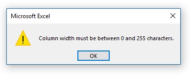
If you try to increase the Column width beyond 255, Excel will show below dialog box.
Two methods for changing the Column width in Excel worksheet are explaind below.
Method 1 — How to change Column width by clicking and dragging on boundary gridline
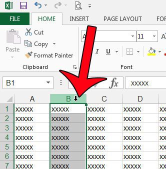
To change the Column width of a single Column by clicking and dragging on Column boundary gridline, follow these steps.
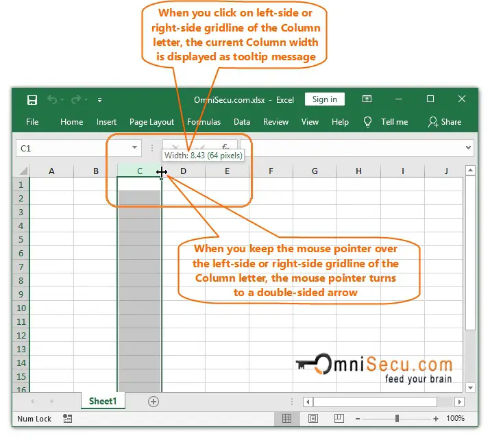
Step 1 — Select the Column you want to change its height by clicking on Column letter. Place the mouse pointer on left-side or righ-side gridline of the Column letter until the mouse pointer turns to a double-sided arrow. You need to place the mouse pointer on left-side or right-side gridline depending on to left or right direction you want to change the Column width. In this example, Column letter C and right-side gridline are selected.
Now click on the right-side gridline of Column letter, as shown below.
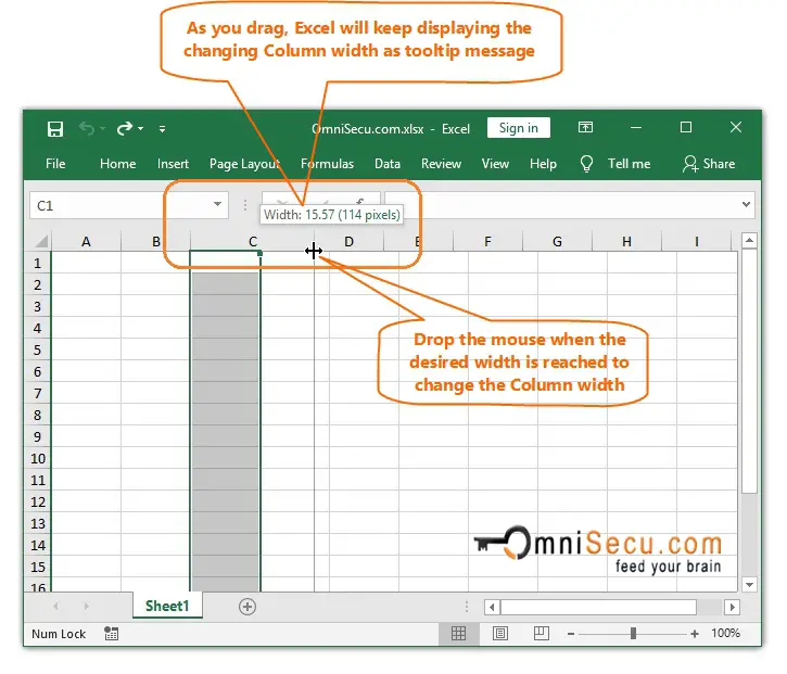
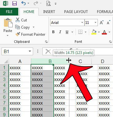
Step 2 — Drag the mouse till the desired width is reached and then drop the mouse to change the Column width. As you drag, Excel will keep displaying the changing Column width as tooltip message.
An animation about how to change the Column width of a single Column by drag and drop is copied below.
.
Similarly, you can change the width of multiple Columns simultaneously by click, drag and drop. Select multiple Columns and then click, drag and drop on left-most or right-most gridline of the Columns selection for changing the width of multiple Columns simultaneously.
An animation about how to change the Column height of multiple Columns by drag and drop is copied below
Method 2 — How to change Column width by entering the exact Column width value
Sometimes it is difficult to select the exact Column width by using drag and drop method described above, because the Column width value keep changing as you drag. Follow below steps to change single Column width by entering the exact Column width value.
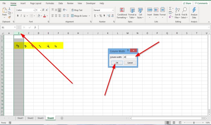
Step 1 — Right-click the the Column you want to change the column width and click the «Column Width» to open «Column Width» dialog box from the context menu, as shown in below image.
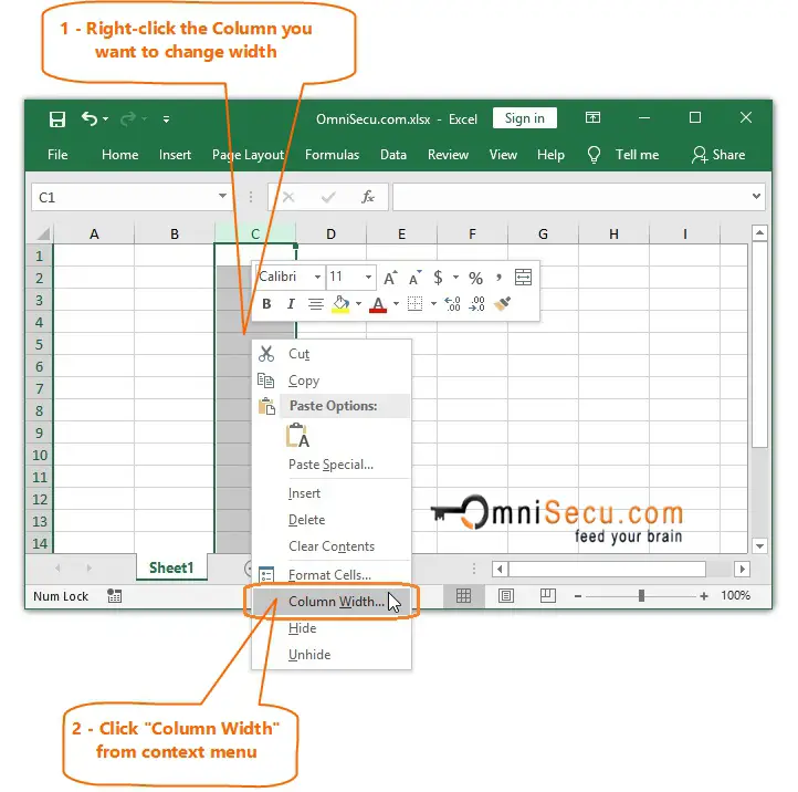
You can open the «Column Width» dialog box also from Excel Ribbon > «Home» Tab > «Cells» > «Format» as shown below.
Step 2 — Enter exact value for Column width in Column width dialog box and click «OK» to change the Column width, as shown below.
Similarly, you can change the width of multiple Columns simultaneously by typing-in the Column width value. Select multiple Columns and then right-click on any Column in the selection. Click the «Column Width» from the context menu and type-in the Column width value in dialog box. Click «OK» button.
Adjusting the column width is one of the important activities while working with Excel. It is one of the important activities performed by a user while preparing the reports, creating dashboards, developing summary tables, and using worksheets to do calculations on data. Microsoft Excel facilitates a set of options for changing the width of the column. However, columns in Excel worksheets cannot automatically adjust the width based on the data.
- A column in Excel has a default width of 8.43 characters, less than one inch. Excel presents different ways, including dragging through a mouse, using the shortcut menus on the ribbon, and double-clicking on the right side edge of the column heading.
- The present article discusses the various effective ways to adjust the width of columns manually by covering the following topics.
Table of contents
- Column Width in Excel
- Explanation
- How to Adjust Column Width in Excel?
- Examples
- Example#1 – Adjusting the Excel Column Width by Using the Mouse
- Example#2 – Setting the Width of the Column to a Certain Number
- Example#3 – Use of Autofit to Adjust the Column Width in Excel
- Example#4 – Setting the Default Width for Columns in Excel
- Things to Remember
- Recommended Articles
Explanation
- In an Excel worksheet, a user can set the width of a column in the range from 0 to 255, and one character width is equal to one unit. For a new Excel sheet, the column width equals 8.43 characters, equal 64 pixels. It will hide a column if its width is equal to zero.
- When a user inputs data into the columns of the excel sheet, they do not automatically adjust the size of the column. If the value presented in a cell is big to fit with the default width of the column, it overlaps with the next cells by crossing the border of the cell.
- The text string cell overlaps the cell border, whereas the numeric string displays in #####. Therefore, we need to apply various commands to adjust the column width to avoid these problems.
In Excel, a different type of command is available to format the width of a column. These include column width, AutoFit column width, and default width.
- Column width: This command sets the width of the column to a certain number of characters.
- Autofit column width: This command helps fit the content to the widest column width.
- Default width: Adjusts column width to the default widthTo autofit the column width to the entire column in Excel, select the entire column and drag the column according to the data. read more.
How to Adjust Column Width in Excel?
- Presenting the data in a readable format adjusting the column width.
- Matching the width of a column in excel to another column.
- Unhide data that is not visible to the readers.
- Setting the specific width to a column to fit with the content produced.
- Application of proper formatting to the cells and their data.
- Precisely controlling the column width by changing the different fonts and their size.
Examples
Below are examples of Excel column width.
You can download this Column Width Excel Template here – Column Width Excel Template
Example#1 – Adjusting the Excel Column Width by Using the Mouse
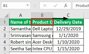
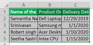
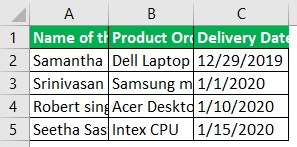
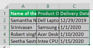
This example illustrates the adjustment of the column width for the following data.

As shown in the figure, data in two columns is not readable. Therefore, we must follow the following steps.
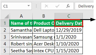
Step1: To adjust the width of only one column, we must drag the border of the column to the right side until the required column width is reached.
Step2: Next, drag the column B width until the desired width is reached.
Step3: Next, we need to drag the column C width until the desired width is reached.
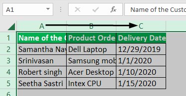
We can adjust the width of all columns by selecting the three columns.
Step4: After that, we must select three columns by pressing “CTRL+A” or clicking the ‘All Button’ and drag on any column header shown in the screenshot.
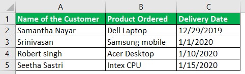
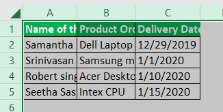
Consequently, it may show the result as follows:
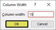
Example#2 – Setting the Width of the Column to a Certain Number
The following data is considered for this example.

We must follow the steps to set the width of a certain number of columns in Excel:
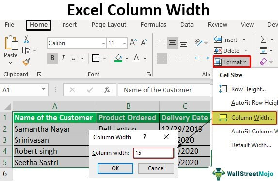
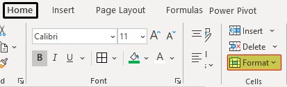
- We must first select the single or more columns to adjust the width.

- Then, go to the “Format” option under the “Home” tab and click on “Format.”

- Next, select the “Column width” from the list of options. It opens the “Column width” dialog box.

- Enter the desired value in the column width box (for example, 15) and click “OK.”
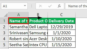
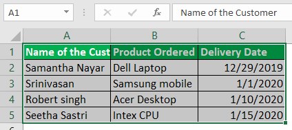
- The result is obtained as follows:

This method results in the same width for the columns selected.
Example#3 – Use of AutoFit to Adjust the Column Width in Excel
This example illustrates the procedure to AutoFit the width of all columns to contents. The following data is considered for this example.
Step1: To AutoFit the single column, first, we need to double-click on the right border of the column.
Step2: To apply the AutoFit to two columns, double-click on the boundary presented by selecting the two columns.
Step3: To apply the AutoFit to all columns, select the columns by pressing “CTRL+A” or selecting the all button.
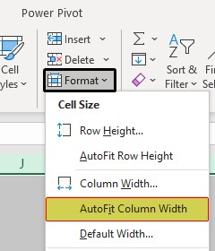
Step4: Go to the “Format” option under the “Home” tab and click on “Format.”

Step5: Select the “AutoFit Column Width” from a list of options as shown in the screenshot.
It AutoFits the width of all columns, as shown in the screenshot.
Example#4 – Setting the Default Width for Columns in Excel
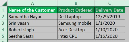
This example illustrates how to change the default column width for a worksheet or complete worksheets in a workbook. The following data is considered for this example.

Step1: First, we must select the single or more worksheets to adjust the default width. For this example, we are considering only one worksheet.
Step2: Go to the “Format” option under the “Home” tab and click on “Format.”
Step3: We need to select the “Default Width” from a list of options, as shown in the screenshot.

It opens the “Standard column width” dialog box.
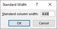
Step4: After that, we must enter the desired width into the “Standard column width” box as 20.
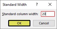
Then, the result is obtained as follows:
Things to Remember
- “AutoFit” of column width does not affect width if the width of the column is sufficient for the content.
- When a user wants to modify the default width of an Excel file, save the empty workbook as a template in Excel.
Recommended Articles
This article is a guide to Excel Column Width. Here, we learn how to adjust the column width in Excel by using the mouse and AutoFit to adjust the column width, along with examples and a downloadable Excel template. You may learn more about Excel from the following articles: –
- Column Total in Excel
- How to Add Columns in Excel?
- Move Columns in Excel
- How to Track Changes in Excel?
Download PC Repair Tool to quickly find & fix Windows errors automatically
The height of rows and the width of columns in Excel are usually automatic, but you can change the row’s height and column width manually. The row height in spreadsheets increases and decreases according to the data’s size entered into the rows; Excel will automatically increase and decrease the rows. Setting the rows’ height is used for specific reasons, such as a cell with an orientation text.
In this tutorial, we will explain how to:
- Change the height of a row.
- Change the width of a column.
What are Rows and Columns in Excel?
- Rows: On the excel Spreadsheet, rows run horizontally. The rows are identified by row numbers which run vertically on the left side of the spreadsheet.
- Columns: On the Excel spreadsheet, columns run vertically and are identified by alphabetical column headers that run horizontally on the spreadsheet’s top.
1] Change the Height of a row
There are two options to change the height of a row.
Option one is to go to where row number three is, place the cursor on the bottom border of the number three-row, hold and drag the cursor down.

You will see the result.
Option two is to click row three.
Then go to the Home tab in the Cells group and click Format.
In the drop-down list, select Row Height

A Row Height dialog box will appear.
Inside the dialog box, place the number of height you want the row to be, then click OK.
2] Change the Width of a column
There are two methods to change the width of the column.
Method one is to go to the right border of column B.
Drag the right border of column B, and you will notice that the column width gets wider.

Method two is to click column B.
Then go to the Home tab in the Cells group and click Format.
In the drop-down list, select Column Width.
A Column Width dialog box will appear; enter the width number you want the column to be and click OK.
I hope this helps; if you have questions, please comment below.
Read next: How to add or remove Borders to Cells in Microsoft Excel.

Shantel has studied Data Operations, Records Management, and Computer Information Systems. She is quite proficient in using Office software. Her goal is to become a Database Administrator or a System Administrator.
-
Excel
Guide to Understanding How to Adjust Column Width in Excel (and Autofit Function)
How to Adjust Column Width in Excel
The following tutorial demonstrates the process of how to adjust the column width in Excel using keyboard shortcuts. Adjusting the column width in a financial model can ensure that all of the necessary data is visible as well as improve the overall presentability of the spreadsheet.

How to Adjust Column Width in Excel (Step-by-Step)
The column width in Excel can be adjusted to sufficiently fit the content within the spreadsheet.
- Narrow Column Width → If the width of a column is too narrow, the value of a cell can become hidden, where the number values appear as “###”.
- Wide Column Width → On the other hand, if the column width is too wide, there could be far too much white space in the spreadsheet, resulting in a distracting appearance. The column width must also be considered if the Excel file will be printed once complete.
By default, the Excel column is set at “8.43 units” with lower and upper parameters of 0 (i.e. hidden) and 255, respectively. The 8.43 units refer to 8.43 characters, which corresponds to 64 pixels, but the units can be adjusted in the settings tab (e.g. into inches, cm, mm).
In the context of financial modeling, it is a general best practice to maintain consistency in the formatting of the column width, albeit there are occasional exceptions.
For instance, most financials models utilize so-called “elevator drops” (i.e. an “x” in a “thinner” Column A) to make the process of navigating between different sections easier.
While there is nothing inherently wrong with one column being of a different width than the rest, a model can appear less professional if each and every column is noticeably set to be a different width.
In order to adjust the column width—either to expand or decrease the width—follow the steps below:
- Step 1 → Select the Column(s) to Adjust
- Step 2 → Open the “Home” Tab
- Step 3 → Click on “Format” to Open the Menu
- Step 4 → Press “Column Width” in the Cell Size Group
- Step 5 → Enter the Specific Width and Click the “OK” Button

If you need to adjust all the columns in the worksheet, simply press “Ctrl” and “A” simultaneously to select all (or click the arrow in the top left corner next to the formula bar), before repeating the same process.
Alternatively, a different method is to select the column to adjust with your cursor, right click to open the menu, and pick the “Adjust Column Width” option.

Whichever method is used, the following box should appear for the user to enter a custom column width.

Adjust Column Width in Excel — Keyboard Shortcut
Using the keyboard rather than the mouse is more time efficient in practically all cases, aside from certain exceptions.
The keyboard shortcut to quickly open the adjust column width box and enter the desired width is as follows.
Adjust Column Width Shortcut = Alt + H + O + W
Each key must be pressed one-by-one in that specific order, instead of pressing down on all of them simultaneously.
Excel Autofit Function: Change Column Width Automatically
Excel also offers the option to adjust the column width automatically to fit the content within the column.
In the “Format” box from earlier, there is a built-in “Autofit Column Width” option to pick from in the cell size group.

If you want to bypass the process of finding and clicking that option, a more convenient approach is to double-click the boundary of a column, i.e. the line separating each column.
Upon doing so, Excel automatically adjusts the column width based on the “best fit”.
Like earlier, selecting all cells and repeating the process on any of the chosen columns auto-adjusts the column width of all the actively selected columns.
Excel Autofit Column Width — Keyboard Shortcut
The preferred option to auto-fit columns, particularly for multiple columns, is to utilize keyboard shortcuts.
The autofit keyboard shortcut is the following:
Autofit Column Width = Alt + H + O + I
As with the shortcut earlier, press each individual key one after the other, and the selected column(s) should be automatically adjusted to display all the included content.
Turbo-charge your time in Excel
Used at top investment banks, Wall Street Prep’s Excel Crash Course will turn you into an advanced Power User and set you apart from your peers.
Learn More
Microsoft Excel has a lot of different tools and settings, many of which allow you to perform the same action in multiple ways. One of the most common things to do in Excel is to change the size of cells, so it only makes sense that there is more than one way to accomplish this. If you are asking what are three ways to change column width in Excel, then our guide below can answer that question.
- Open your spreadsheet.
- Select the column.
- Right-click on the column and choose Column Width.
- Enter the new width, then click the OK button.
Our guide continues below with additional information to answer the question of what are three ways to change column width in Excel, including pictures of these steps.
The heights of rows and widths of columns in an Excel spreadsheet are the same size in every new spreadsheet that you create. But the data that you put into your cells can vary in size, and you may find that the default cell sizes are often too small or too large.
Fortunately, the sizes of your cells are elements that can be adjusted, and modifying your column widths is a simple task that will make your spreadsheet easier to read and work with.
So continue reading below to learn about several different methods that you can use to change the widths of your columns in Excel.
Did you know that there is also a method for how to expand rows in Excel? This can be useful when you have multiple lines of data inside of your cells and want it all to be visible.
How to Adjust Column Width in Excel 2013 (Guide with Pictures)
This article was written using Excel 2013, but the same steps can be applied in other versions of Excel as well. Additionally, you can follow similar steps if you need to adjust the height of your rows.
There are three different ways to adjust column widths that are discussed below. Choose the best option based on your spreadsheet needs.
Method 1 – Manually Resize Column Width
This option is best used if you wish to visually modify the width of your columns.
Step 1: Open your spreadsheet in Excel 2013.
Step 2: Locate the column whose width you wish to adjust.
Step 3: Click the right border of the column letter, then drag it left or right to the desired width.
Method 2 – Numerically Resize Column Width
This option is best used if you want to make sure that all of your column widths are the same size. You can also use this option with multiple selected columns.
Step 1: Open your spreadsheet in Excel 2013.
Step 2: Right-click the column letter that you want to change, then click the Column Width option.
Step 3: Enter a new value inside the Column Width field, then click the OK button.
If you are not able to use right-click, then you can find the Column Width option by clicking the Home tab at the top of the window, clicking the Format button in the Cells section of the navigational ribbon, then clicking the Column Width option.
Method 3 – Resizing the Column Width Based on the Width of the Cell Contents
This option is best used when you simply want all of the data contained within a column to be visible.
Step 1: Open your spreadsheet in Excel 2013.
Step 2: Click the column letter of the column whose width you want to adjust automatically.
Step 3: Position your mouse cursor on the right border of the column, then double-click your mouse. The column will automatically adjust itself to fit the size of the data contained within it. This can make your column widths smaller or larger, depending upon your data.
Are there multiple columns in your spreadsheet that you would like to resize to fit their contents? Learn how to autofit column widths in Excel with just a few button clicks.
Additional Sources

Matthew Burleigh has been writing tech tutorials since 2008. His writing has appeared on dozens of different websites and been read over 50 million times.
After receiving his Bachelor’s and Master’s degrees in Computer Science he spent several years working in IT management for small businesses. However, he now works full time writing content online and creating websites.
His main writing topics include iPhones, Microsoft Office, Google Apps, Android, and Photoshop, but he has also written about many other tech topics as well.
Read his full bio here.
Do you spend a lot of time changing the column width in Excel? On the one hand, you’d like to see as many columns as possible for having a good overview. On the other hand, you want to see as much content as possible within a column. In the worst case, you’d only see ### instead of values. Let’s have a look at how to adjust the rows and columns of an Excel sheet.
Method 1: Distribute rows and columns manually
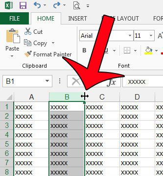
The first method is the most intuitive one: Manually per drag and drop to adjust the width of each column.
Just click on the small column (or row) divider as shown in the image on the right side. Hold the mouse down and move it in the direction you want.
This way also works if you select many columns (or rows) at the same time. All columns get the same width then.
Tip: If there are hidden columns in between, you can unhide them by selecting all columns from the left to right column of the hidden column. Then change the column width for just one column and all of them (also the previously hidden column) get the same width.
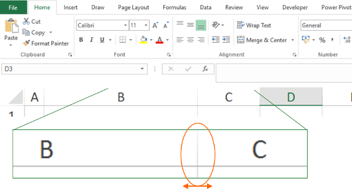
Method 2: Double click for automatic sizing the whole column
A faster way is to double click on the divider between columns (or rows). Double click on the line between the column letters on the top of the window can find the smallest possible width.
There is a keyboard shortcut combination for adjusting the column width:
- Select the complete column with Ctrl + Space on the keyboard.
- Press the following keys after each other: Alt –> H –> O –> I.
The keyboard shortcut for rows is quite similar:
- Select the row with Shift + Space.
- Press Alt –> H –> O –> A after each other.
Alternatively you can go to “Home” –> “Format” (under “Cells”) –> “AutoFit Column Width” or “AutoFit Row Height”.
Please note: That way, the column width (or row height) will adapt to the contents of the complete column (or row).
Method 3: Adjust the column width for only the selected cell content
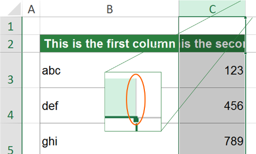
Please take a look at the example on the right side. You got a table in the cell range B2 to C7. Below, in cell B9 is a footnote, which is quite long.
You want to adjust the column width to fit the upper table, B2 to C7 in it.
It’s quite similar to our method 2 above. The only exeption: Instead of adjusting the entire column, just select the cell range B2:C7.
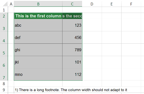
Now apply the keyboard shortcut from above: Alt –> H –> O –> I. Alternatively, click “Home” –> “Format” (under “Cells”) –> “AutoFit Column Width”.
If you want to do the same for the row it, use the following methods after selecting all the rows:
- Press Alt –> H –> O –> A on the keyboard after each other.
- Go to “Home” –> “Format” (under “Cells”) –> “AutoFit Row Height”
Do you want to boost your productivity in Excel?
Get the Professor Excel ribbon!

Add more than 120 great features to Excel!
Method 4: Adjust the column or row width with a fixed value
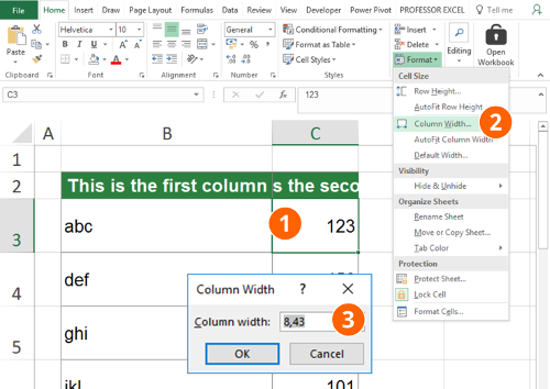
The previous methods aren’t exact enough for you? Then please consider this way.
You can set a specific column width (or row).
- Select a cell within the column (or row) you want to adjust.
- Click on “Format” on the “Home” ribbon and then on “Column Width…” (or “Row Height…”).
- Type your desired value and confirm with OK.
Please note: The value you type represents the number of characters shown in the standard font. “0” means, that the column (or row) is hidden.
Troubleshooting
How to deal with a column width larger than the screen?
This might happen, if you automatically distribute columns. The easiest way to solve this: Set a specific column width (e.g. “8”) according to the steps in method 4.
What if you can’t change the column width?
There are several possible reasons if you can’t change the column width. Please check the following:
- Another window is open (maybe in the background).
- The sheet is locked for editing. If yes, click on unlock.
- The workbook is not enabled for editing (is there s yellow bar on top of the rows?).
- You are editing a cell content (also in another window of Excel possible). Press Enter of Esc for leaving the cell.
The column is not shown (e.g. column A) and you can’t scroll to it?
Does your worksheet have frozen panes? If yes, unfreeze them by clicking “View” –> “Freeze Panes” –> “Unfreeze Panes”.