
Excel for Microsoft 365 Excel 2021 Excel 2019 Excel 2016 Excel 2013 More…Less
To change the text fonts, colors, or general look of objects in all worksheets of your workbook quickly, try switching to another theme or customizing a theme to meet your needs. If you like a specific theme, you can make it the default for all new workbooks.
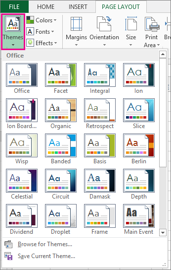
To switch to another theme, click Page Layout > Themes, and pick the one you want.
To customize that theme, you can change its colors, fonts, and effects as needed, save them with the current theme, and make it the default theme for all new workbooks if you want.
Change theme colors
Picking a different theme color palette or changing its colors will affect the available colors in the color picker and the colors you’ve used in your workbook.
-
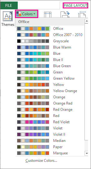
Click Page Layout > Colors, and pick the set of colors you want.
The first set of colors is used in the current theme.

-
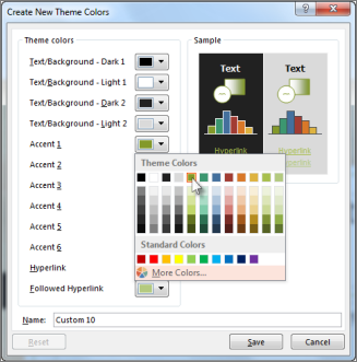
To create your own set of colors, click Customize Colors.
-
For each theme color you want to change, click the button next to that color, and pick a color under Theme Colors.
To add your own color, click More Colors, and then pick a color on the Standard tab or enter numbers on the Custom tab.
Tip: In the Sample box, you get a preview of the changes you made.
-
In the Name box, type a name for the new color set, and click Save.
Tip: You can click Reset before you click Save if you want to return to the original colors.
-
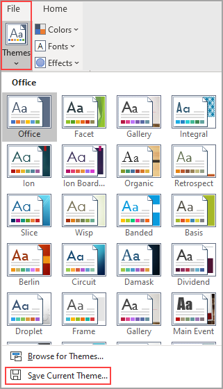
To save these new theme colors with the current theme, click Page Layout > Themes > Save Current Theme.
Change theme fonts
Picking a different theme font lets you change your text at once. For this to work, make sure Body and Heading fonts are used to format your text.
-
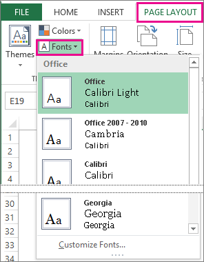
Click Page Layout > Fonts, and pick the set of fonts you want.
The first set of fonts is used in the current theme.
-
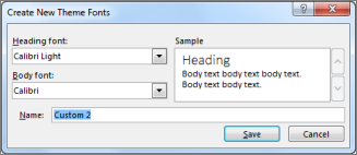
To create you own set of fonts, click Customize Fonts.
-
In the Create New Theme Fonts box, in the Heading font and Body font boxes, pick the fonts you want.
-
In the Name box, type a name for the new font set, and click Save.
-
To save these new theme fonts with the current theme, click Page Layout > Themes > Save Current Theme.
Change theme effects
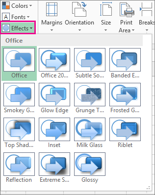
Picking a different set of effects changes the look of the objects you used in your worksheet by applying different types of borders and visual effects like shading and shadows.
-
Click Page Layout > Effects, and pick the set of effects you want.
The first set of effects is used in the current theme.
Note: You can’t customize a set of effects.
-
To save the effects you selected with the current theme, click Page Layout > Themes > Save Current Theme.
Save a custom theme for reuse
After making changes to your theme, you can save it to use it again.
-
Click Page Layout > Themes > Save Current Theme.
-
In the File name box, type a name for the theme, and click Save.
Note: The theme is saved as a theme file (.thmx) in the Document Themes folder on your local drive and is automatically added to the list of custom themes that appear when you click Themes.
Use a custom theme as the default for new workbooks
To use your custom theme for all new workbooks, apply it to a blank workbook and then save it as a template named Book.xltx in the XLStart folder (typically C:Usersuser nameAppDataLocalMicrosoftExcelXLStart).
To set up Excel so it automatically opens a new workbook that uses Book.xltx:
-
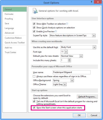
Click File>Options.
-
On the General tab, under Start up options, uncheck the Show the Start screen when this application starts box.
The next time you start Excel, it opens a workbook that uses Book.xltx.
Tip: Pressing Ctrl+N will also create a new workbook that uses Book.xltx.
Need more help?
Every workbook uses a palette of 56 colors, but you can change the palette for the current workbook or even
change the default colors for new workbooks.
To change the colors of the current workbook
1. On the Page Layout tab, in the Themes
group, click Theme Colors:

2. Click Customize Colors…:

3. In the Create New Theme Colors dialog box, under
Theme colors, click the button of the theme color element that you want to change:

4. Under Theme colors, select the colors that you
want to use:

In the Create New Theme Colors dialog box, under Sample, you can see the effect of the
changes that you make.
5. Repeat steps 3 and 4 for all of the theme color elements
that you want to change.
6. In the Name box, type an appropriate name for the
new theme colors.
7. Click Save.
Note: To revert all theme color elements to their original theme colors, you can click
Reset before you click Save.
To make changes apply to all new workbooks
If you would like to make these color changes apply to all new workbooks that you create, you
need to create a default workbook template.
1. On the Page Layout tab, in the Themes
group, click Themes.
2. Click Save Current Theme…:

3. In the File Name box, type an appropriate name for
the theme.
Note: A customs document theme is saved in the Document Themes folder and is
automatically added to the list of custom themes.
4. On the File tab, choose Save As.
5. In the Save Current Theme dialog box, was selected
Office Theme (*.thmx) and chose the Document Themes folder as the location. You
can use your own filename instead of the proposed Theme1.thmx.
The location of the Document Themes folder may vary, but it is usually located here:
C:Users<user name>AppDataRoamingMicrosoftTemplatesDocument Themes
6. Click Save.
See also this tip in French:
Comment modifier les couleurs par défaut qu’Excel utilise pour les séries de graphiques.

Color in Excel (Table of Contents)
- Introduction to Color in Excel
- Ways to Change Background Color
Introduction to Color in Excel
Colors are generally used to highlight a group of cells in Excel. The excel contains the index of 56 colors. By using conditional formatting, we can put some conditions and apply different colors for different conditions if we want to change the background color of the cell in Excel. We usually select the cells and click the Fill color option; then, the background color will get changed if we want to change the cell’s background colour with the cell automatically.
Ways to Change Background Color
There are two ways to change the background color.
You can download this Color Excel Template here – Color Excel Template
1. Change the color of the cell based on the current value
- Here the background color of the cell changes when the cell value in the Excel changes.
- For example, we have taken the following dataset. we want the USD Amount greater than 10,000 as blue color and remaining red color.

- Select the range of the cells which we want to change. Then go to the Home tab, go to the styles and select the conditional formatting.

- Now click on the new rules.
- A dialog appears stating the selection of the row. Select the format of the cells based on the cell value.

- Now give the range of values which are greater than 10,000 and select the color as blue color.


- Now click on the format option.
- A color box appears and makes the Pattern Color as Automatic, so Select color as blue and click on OK.

- We can observe that the sample option is blue because we have selected the blue color.

- We can observe the selected color in the format option. And click the Ok option.

- Now we can use the same procedure for selecting the color for less value. A dialog appears stating the selection of the row. Select the format of the cells based on the cell value. A dialog appears stating the selection of the row. Select the format of the cells based on the cell value. Now give the range of values which are less than 10,000 and select the color as red color.

- The color box appears and makes the pattern as automatic and Select color like blue and click OK.
- The output will be as follows.

2. Change the background color of special cells
- This is another way of color the background of the particular cell. First, go to the home tab, then select the conditional formatting.

- Select the new rules.
- The formatting dialog box appears to click on the cells which need to format, which is at the end of the dialog box.

- Click on the arrow option at the right end.
- Write the new formatting rule using the keyword Is Blank condition. This Is Blank is used to highlighting the background cells which are empty.

- Click on the Format option. And select the blue color.

- Click on the Ok button.

- The output will be as follows.

3. Sort the Excel by it Color
- Sorting is one of the methods to select a particular color. First, select the cells, right-click on them, select the sort option, and then select the highest value by color.

- Click the ok button.
- And Filter the color by its color.


- And the output will be as follows.
Change the cell color based on the current value.
- First, go to the home tab, select the Find and select option, and select the Find option.
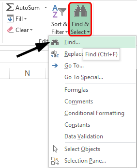
- Select the value which we want to select. Click on the Find all option.
- Click on the values range which we want the cells we want to highlight.
- Click on the Select by value option. And select the Greater in the list.
- Click on the range of the cells we want to highlight. Click on the select option.
- Now select the color as blue for the greater value.
- And the output will be as follows.
Conditional Formatting in Excel
- Conditional formatting is generally used to color data bars and icons in the cells.
- To do the conditional formatting in Excel, first, we take the required data set.
- Then go to the Home tab and select the conditional formatting option ad put the desired rule which we want to specify, and mention the color which we want to give to the cells of the particular condition.
- Then a dialog box appears on the screen then simply gives the values we want a particular condition so that the color will be applied successfully.
- Now select the formatting styles from the drop-down. Here we select the color for the condition. Then click the OK. The conditional formatting will be applied to all the cells at a time. This is one way of adding colors to the cells.
Things to Remember About Color in Excel
- The colors in excel play a major role in highlighting a particular range of cells.
- Here we generally use the two approaches like make the background color cells based on the value, and another way is to change the background of special cells.
- The excel contains the index of 56 colors. By using conditional formatting, we can put some conditions and apply different colors for different conditions.
- We can also sort the colors based on the colors.
- We can highlight the empty cells with the colors.
- Through cells, we can highlight the greater values and the lower value with different colors.
Recommended Articles
This has been a guide to Color in Excel. Here we discuss How to use Color in Excel along with practical examples and a downloadable excel template. You can also go through our other suggested articles –
- Alternate Row Color Excel
- Excel Sum by Color
- Count Colored Cells In Excel
- Excel Sort by color
In this lesson we will learn how to change the color of a table in Excel. For this, we will initialize the original table from the previous lesson by formatting the background and cell borders.
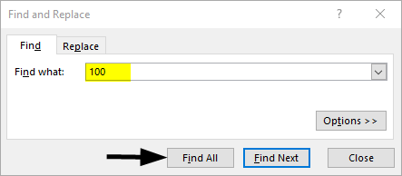
Immediately go over to practice. We select the whole table A1:D4.
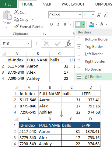
On the «Home» tab, click on the «Borders» tool, which is located in the «Font» section. From the drop-down list, select the option «All borders».
Now again in the same list, select the option «Thick outer border». Next, select the range A1:D1. In the same section of the tools, click on «Fill color» and point to «Dark Blue». Next, in the «Text color» tool, point «White».
The example of changing the color of tables
The pictures show the process of changing the boundaries in practice:
You can also change the color of a table in Excel using the more functional tool.
Select again the entire table A1:D4. Press the hotkey combination CTRL + 1 or CTRL + SHIFT + F. The multifunction dialog box «Format Cells» will appear.
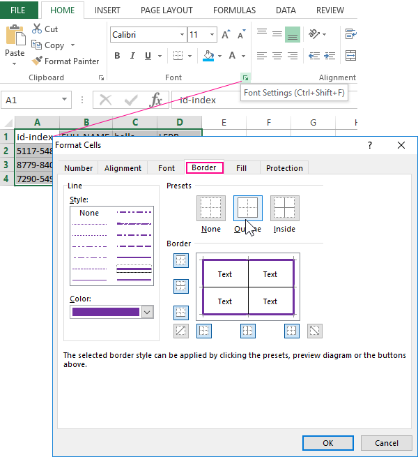
First go to the «Border» tab. In the «Presets» toolbar of this tab, click the «Inside» button. Now in the line type section, select the thickest line (second from the bottom in the right column). If necessary, set the color for the borders of the table below. Then go back to the «All» section and click on the «Outline» button. To confirm the border formatting settings, click OK.
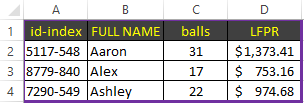
Also we can make a colors text. Select the headings of the original table A1:D1. Open the «Format Cells» window. At present go to the «Font» tab and in the text color field select «Yellow». To change the color of the selected cell in Excel, click the «Fill» tab and click on «Black». To confirm the change of the format of the cells, click OK. Pasting cells in Excel allows you to select a row or column by color.
As you can see in the «Format Cells» window there are multiplicity of tools, that expand the possibilities of formatting data.
The helpful advice! Format the data in the last place: so you will save your working time.
The formatting opens up wide possibilities for data exposure. There are the changing fonts and sizes of text, setting background colors and patterns, paint border colors and select the type of their lines, etc. But if you slightly overdo with the color change a little, the Excel sheet becomes colorful and unreadable.
Do you need to change the sheet tab colors in your workbook? This post is going to show you all the ways to change the tab color of your sheets in Microsoft Excel.
Excel lets you customize your workbooks in a variety of ways. One popular way to visually organize your worksheets is to change the color of the sheet tabs.
Using different colors for sheets that contain inputs, data, calculations, reports, or visuals can be a helpful way to arrange your workbooks. You might also have a sheet for each month of the year and distinguish each quarter by color.
Excel makes it easy to change tab colors, and doing so can help users keep track of important information.
By changing the tab color, users can quickly identify which sheets contain what type of information.
Get your copy of the example workbook used in this post and follow along!
Change the Sheet Tab Color with a Right Click
The most straightforward way to change your sheet tab color is with the right-click menu.
When you right-click on any sheet tab, you will see various options including changing the color.
Follow these steps to change your sheet tab color.
- Right-click on the sheet tab to which you want to change the color.
- Select the Tab Color option from the menu.
- Choose a color option.
Your sheet tab will now be colored.
📝 Note: the color that is displayed on the tab will usually be a lighter shade than the chosen color while the tab is selected. Select any other tab and the chosen color will be prominently displayed.
If you want more selection than the Standard Colors or Theme Colors, you can select the More Colors option.
This will open the Colors menu and you will be able to more precisely pick your color from a color map or provide the exact RGB or Hex code for the color.
Remove the Sheet Tab Color a Right Click
If you need to remove any coloring you’ve applied to your tab, you can also do this with the right-click menu.
Follow these steps to remove the color from a tab.
- Right-click on the sheet from which you want to remove the color.
- Choose Tab Color from the options.
- Chose No Color from the options.
The color is removed from your selected tab!
Change the Sheet Tab Color with the Home Tab
These color tab options are also available in the Home tab of the ribbon.
Follow these steps to change the sheet tab color from the Home tab.
- Select the sheet to which you want to change the tab color. It should be the active sheet in the workbook.
- Go to the Home tab or the ribbon.
- Click on the Format command found in the Cells section.
- Choose the Tab Color option from the menu.
- Choose your desired color.
Your active sheet tab will now be colored with the chosen color!
Change the Sheet Tab Color with a Keyboard Shortcut
There is no dedicated keyboard shortcut for changing the tab colors, but you can access the Tab Color menu by using the Alt hotkey shortcuts.
Press the Alt key and the ribbon will show you what key will access the different commands in the ribbon.
Press the Alt, H, O, T sequence to open the Tab Color options menu.
- Pressing Alt will activate the hotkeys.
- Pressing H will select the Home tab in the ribbon.
- Pressing O will select the Format command from the Cells section.
- Pressing T will open the Tab Color menu.
Once you have the Tab Color menu open, you can use the arrow keys to select a color option. Press the Enter key to confirm the color choice and change your tab color.
You can also press the M key at any time for the More Colors menu.
Change Multiple Sheet Tab Colors at the Same Time
If you need to change the color or many sheets, you definitely wouldn’t want to do it manually for each sheet. That would take a lot of clicks!
Thankfully, you can change the color of multiple sheet tabs at once!
Change Multiple Adjacent Sheet Tab Colors
You can select multiple adjacent tabs and then change the color.
- Select the first tab.
- Hold the Shift key.
- Select the last tab.
- Right-click on the last tab.
- Choose the Tab Color option from the menu.
- Choose the color for all your selected tabs.
All the selected tab colors are changed!
Change Multiple Non-Adjacent Sheet Tab Colors
You can select multiple non-adjacent tabs and then change the color.
- Select the first tab.
- Hold the Ctrl key.
- Select any other tabs.
- Right-click on the last tab.
- Choose the Tab Color option from the menu.
- Choose the color for all your selected tabs.
All the selected tab colors are changed!
Change All Sheet Tab Colors
There is a quick way to select all the tabs in your workbook. You can then change the color for all the selected sheets.
- Right-click on any tab.
- Choose the Select All Sheets option from the menu.
- Right-click on any sheet.
- Choose the Tab Color option from the menu.
- Choose the color for all your selected tabs.
Now all the sheet tab colors have been changed!
💡 Tip: This is a great way to change all but one or two tab colors. After all the sheets are selected, hold the Ctrl key and click on any tab to deselect it.
Change the Sheet Tab Color with VBA
Changing the sheet tab color is something you can automate!
Suppose you want to change the tab color for all sheets named with a certain prefix. You can get this done with a bit of VBA code.
Go to the Developer tab and select the Visual Basic command to open the visual basic editor. You can also press the Alt + F11 keyboard shortcut to open the VBA editor.
💡 Tip: Check out this post to learn how to show the Developer tab in your ribbon.
Go to the Insert menu in the editor and select the Module option.
Sub ChangeTabColor()
Dim ws As Worksheet
    For Each ws In ThisWorkbook.Worksheets
        If Left(ws.Name, 4) = "2021" Then
            ws.Tab.Color = RGB(0, 176, 80)
        End If
    Next ws
End Sub
Now you can paste the above code into the new module.
This code will loop through each sheet in the workbook and check if the sheet name starts with 2021, and if so, the tab color is changed. Otherwise, nothing is changed.
The color is set based on the RGB code and these values can be changed as needed to achieve different colors.
You can also adjust the "2021" in the above code to whatever text you need. For example, Left(ws.Name, 1) = "A" would check if the sheet name started with A.
When you run this VBA code, all the matching sheets will get their color updated.
Remove the Sheet Tab Color with VBA
You can also remove the tab color using VBA code.
All you need to do is change this line of code ws.Tab.Color = RGB(0, 176, 80) with this line ws.Tab.Color = False.
This will set the tab color to No Color.
Change the Sheet Tab Color with Office Scripts
Office Scripts is a JavaScript language for Excel but is only available in the web version with a Microsoft 365 business subscription.
If you are using Excel online and need to automate your tasks, this is the tool you need!
You can also automate your tab color changes with Office Scripts.
Go to the Automate tab in Excel online and select the New Script command.
function main(workbook: ExcelScript.Workbook) {
	let sheets = workbook.getWorksheets();

	for (let sheet of sheets) {
		if (sheet.getName().startsWith('2021')) {
			sheet.setTabColor('FF0000');
		};
	};
}
This will open the Office Scripts Code Editor and you can place the above code and press the Save script button.
This code loops through all the sheets in the workbook and will change the tab color if the sheet name starts with 2021. It will change the tab color based on the hexadecimal color code supplied in the code.
In this example, the hex code is FF0000 so the tabs will be updated with a red color, but you can change this hex code based on your needs.
Remove the Sheet Tab Color with Office Scripts
You can also remove any tab colors that have been applied to your workbook with a slight change to the code.
Replace this line of code sheet.setTabColor('FF0000'); with this line sheet.setTabColor('');.
This will set the tab color to No Color.
Conclusions
Changing the sheet tab color is a great way to visually organize your Excel spreadsheets.
There are several ways to manually change the color from the right-click menu, Home tab, and using the hotkey shortcuts.
Changing multiple sheet colors at the same time is also possible. You can select multiple sheets and then change the color for all that are selected.
The colors on your sheet tabs can also be automated through VBA and Office Scripts when you need to deal with many sheets or you need to color code sheets in many workbooks.
Do you use this tab color feature? Do you know any other tips for changing the sheet tab colors? Let me know in the comments below!
About the Author
John is a Microsoft MVP and qualified actuary with over 15 years of experience. He has worked in a variety of industries, including insurance, ad tech, and most recently Power Platform consulting. He is a keen problem solver and has a passion for using technology to make businesses more efficient.
Based on certain values in our worksheet, we might decide to format the sheet by assigning colors based on values. In this tutorial, we will explore how to change color in excel based on values in Excel 2013, 2010 and 2016. We will also learn how to use Excel formulas to change the background colors of cells with formula errors or blank cells.
 Figure 1 – How to change cell color based on the value
How to Change Cell Color Based On Value with Conditional Formatting
When we have a table and wish to change the color of certain cells dynamically, Excel conditional formatting is a great tool we can use. It will help us highlight the values less than Y, greater than X or between X and Y. To begin:
- We will select the table or range where we want to change the background color of cells. Here we have selected the entire table.
- Now, we will go to the Home tab, select styles group and choose Conditional formatting
 Figure 2 – Formula for changing color
- We will select New Rule and in the New Formatting Rule dialog box, under the Select a Rule type box, we can select any rule. For now, we will select “Format Only Cells that contain”.
- In the lower part of the dialog box, where we have Format Only Cells with section, we will set the rule conditions. Next, we will choose to format only cells with a cell value between 90 and 140.
 Figure 3 – New formatting rule dialog box
- Now, we will click the Format button and choose the background color we want to apply
- In the Format Cells dialog box, we will switch to the fill tab and pick the color we want. Next, we click OK.
 Figure 4 – How to change font color based on the value
- We will be redirected back to the New Formatting Rule window. Here, we will preview the format changes in the Preview box. Once we are satisfied with everything, we will click OK.
 Figure 5 – How to change color
How to Change the Background Color for Special Cells (cells with formula errors or blanks)
- In the Home tab, we will go to the Styles group and click Conditional formatting
- Next, we will select New Rule. In the New Formatting Rule dialog, we will select the option Use a formula to determine which cells to format.
- Now, we will enter one of the following formulas in the format values where this formula is true field. In our example, we will select the formula for changing the color of blank cells
=IsBlank() – to change the background color of blank cells.
=IsError() – to change the background color of cells with formulas that return errors.
Where () should contain the highlighted cells.
 Figure 6 – Color cell based on the value of another cell
- Alternatively, we can click on Format only Cells that contain and select Blanks in the lower end of the dialog box.
 Figure 7 – Color cell based on the value of another cell
- We will select the Format button and choose the background color we want in the fill Tab.
 Figure 8 – How to change font color based on the value
- In the Format Cells dialog box, we will switch to the fill tab and pick the color we want. Next, we will click OK.
- We will be redirected back to the New Formatting Rule window. Here we will preview the format changes in the Preview box. Once we are satisfied with everything, we will click OK.
 Figure 9 – How to excel change cell based on the value of another cell.
Instant Connection to an Excel Expert
Most of the time, the problem you will need to solve will be more complex than a simple application of a formula or function. If you want to save hours of research and frustration, try our live Excelchat service! Our Excel Experts are available 24/7 to answer any Excel question you may have. We guarantee a connection within 30 seconds and a customized solution within 20 minutes.
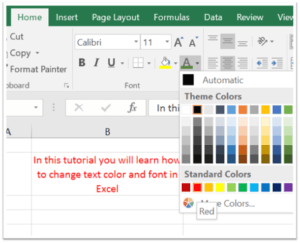
Have you ever thought to change text color and font in Excel?
Till now, we are only aware of how to change color and font for the entire cell contents.
Yes, right? But, sometimes you would be needed to change text color and font. I mean changing the color and text to little piece of the text. Do you know how to do it or ever thought of doing so?
Do not worry. Our very own Excel expert Szilvia Juhasz lets us know how to do it simply. The trick to change text color and font is really useful, attractive and mostly very simple.
What are you waiting for?
First, rather than jumping in to the trick, let us look at how to color contents in a cell.
1 – How to Change Color and Font of a Cell Contents in Excel
- You just need to select the cell which you are interested in.
- Click on the ‘Home’ tab and then under ‘Font’ section, click on ‘Font Color’ to select the color you want to apply to the cell contents.
- To change the font and font size, select the font and font size which you want from the font and font size dropdowns respectively.
 Did you see that?
Color, font and font size got applied to all contents of the cell. This is the general and straight forward way to change color and font in Excel. This is what we know and what we are doing till now. Now, the actual trick comes in to the picture. Let us see, how we can change text color and font in Excel rather than whole contents of the cell.
The actual technique follows as,
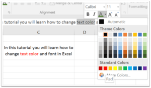
2 – The Trick to Change Text Color and Font in Excel
Changing text color and font in Excel can be done in two simple steps as follows,
- First select the cell you want and select the particular text in the formula bar which you want to color.
- Click on the ‘Font Color’ of ‘Font’ section under ‘Home’ tab. Next, select the color which you want to apply.
- Hurray! Only selected piece got selected. Now, if you want to change the font or font style you can select the font from the ‘Font’ dropdown under the same ‘Home’ tab.
- You can even apply these changes by right clicking on the selected text.

These are the simple steps to change text color and font in Excel. Now you could see that, only particular text of the cell contents is colored.
Amazing Trick! Thanks Szilvia Juhasz for this interesting trick.
3 – Advantage of this Trick
This trick can be used when you want users to input values to the Excel. Let us take an example of an Excel which has VBA Code taking SQL Query as it’s input. Let us say that SQL Query has two attributes ‘StartDate’ and ‘EndDate’. To warn the users that, they need to provide these two values to run the VBA, you can add red color to these texts in the Query. In this way, users will be aware that they need to input these values to proceed further.
What’s next?
Give it a try buddies! Also, if you have any excel tips or want to add anything to this trick, please do share with us through comments.
Share this trick with your friends and colleagues. Enjoy the trick!
There are several ways to change the worksheet tab colour by using the shortcut keys or other commands in excel. Changing the worksheet tabs’ colours helps us to understand the difference between the tabs of different works easily. So, follow one of the 5 methods you like.
Table of Contents
- 1. Change Worksheet Tab Color in Excel
- 2. Change Worksheet Tab Color from Home Tab
- 3. Change Worksheet Tab Color in Excel
- Change All Sheet Tab Color at a Time:
- Remove All Sheet Tab Colors at a Time:
- 4. Using Alt Key
- 5. Change Sheet Tab Color Using VBA
Right-click on the “Sheet tab”, which appears at the bottom right corner of the excel workbook as given in the picture below.
Then move your cursor on the “Tab colour”, and then immediately a Color dialogue box appears
Now you can select one of the Theme Colors or the Standard Colors you want
If you want to remove the Color of a Sheet tab, Select “No Color”.

2. Change Worksheet Tab Color from Home Tab
Go to the Home tab
Then click on the drop-down arrow of the Format in the Cells group
Afterwards, move your cursor on the “Tab colour”, and then immediately a Color dialogue box appears
Now you can select one of the Theme Colors or the Standard Colors you want
Look at the 5th step of the picture below.
If you want to remove the Color of a Sheet tab, Select “No Color”.

3. Change Worksheet Tab Color in Excel
Change All Sheet Tab Color at a Time:
To change all the Sheet tab colours at a time, Right click on the “Sheet tab”, which appears at the bottom right corner of the excel workbook as given in the picture below.
Then click “Select All Sheets”

Again, right-click on the “Sheet tab”
Then move your cursor on the “Tab colour”, and then immediately a Color dialogue box appears
Now you can select one of the Theme Colors or the Standard Colors you want

Remove All Sheet Tab Colors at a Time:
If you want to remove the colour of all the sheet tabs at a time, do the following.
Right-click on the “Sheet tab”
After that, click “Select All Sheets”

Again, right-click on the “Sheet tab”,
Now if you move the cursor on the “Tab colour”, immediately a Color dialogue box appears
Finally, Select “No Color”.
4. Using Alt Key
Press Alt + H → O → T, and Select one of the Theme Colors or Standard Colors you want.

5. Change Sheet Tab Color Using VBA
VBA stands for Visual Basic for Applications. It is a programming language developed and owned by Microsoft Corporation. It is used to create custom reports, forms, graphs and more. You can change the worksheet tab colour using VBA.
What is the benefit of changing the worksheet tab colour in Excel?
Changing the worksheet tabs’ colours helps us to understand the difference between the tabs of different works easily.
Today we’re gonna talk about how to change chart colour in Excel. This can be especially helpful if you need the colour of the bars in a chart to match your presentation theme, but also any time you need to use a colour different from the default one.
Ready to start?
Would you rather watch this tutorial? Click the play button below!
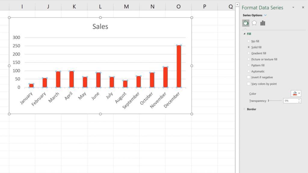
To change chart colour, first we double-click on any bar in the chart.
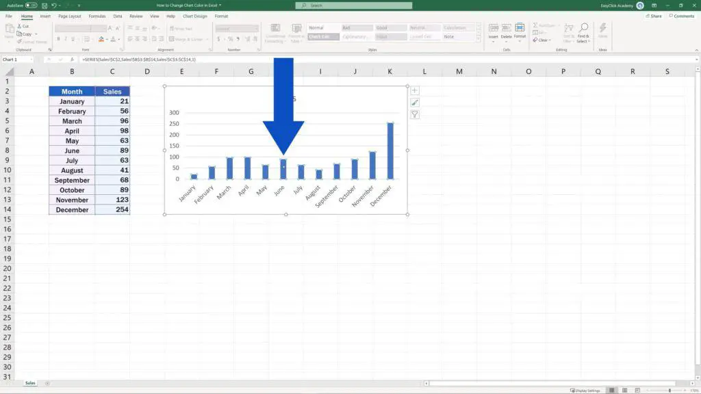
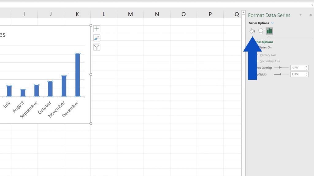
On our right, we can see a pane with various options to format data series.
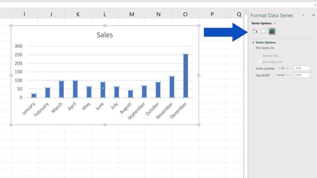
In this tutorial, we’re going to cover only how to change chart colour, so click on the option Fill & Line.
Here you can choose a colour fill for the bars as well as the border type.
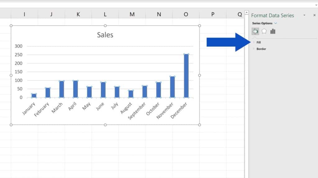
Let’s have a look at both options one by one.
How to Change a Colour Fill for the Bars
Expand ‘Fill’ and the menu that appears offers several options you can apply, like ‘No fill’, ‘Solid fill’ or ‘Gradient fill’ among many others.
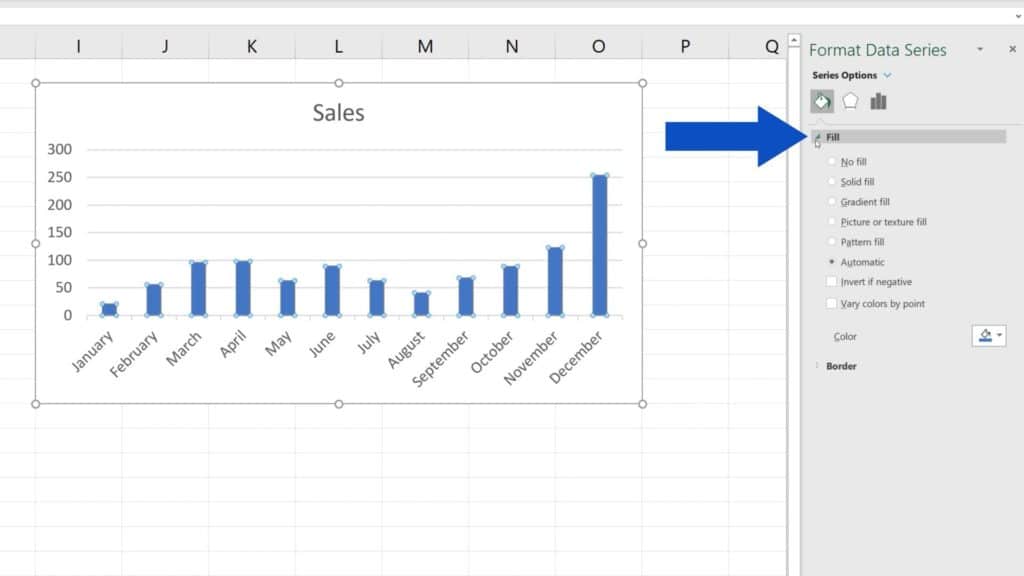
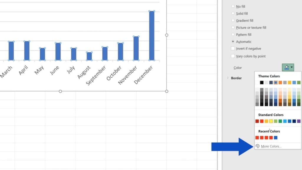
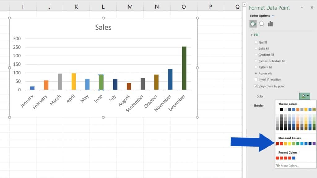
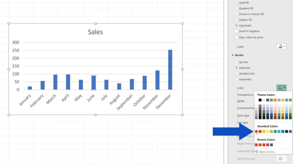
To change the default blue in all the chart bars, click on the icon next to ‘Colour’ and choose any of the pre-defined, standard colours offered here.
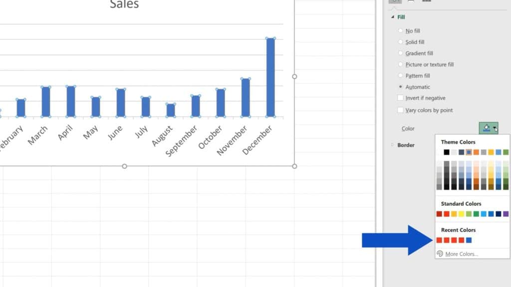
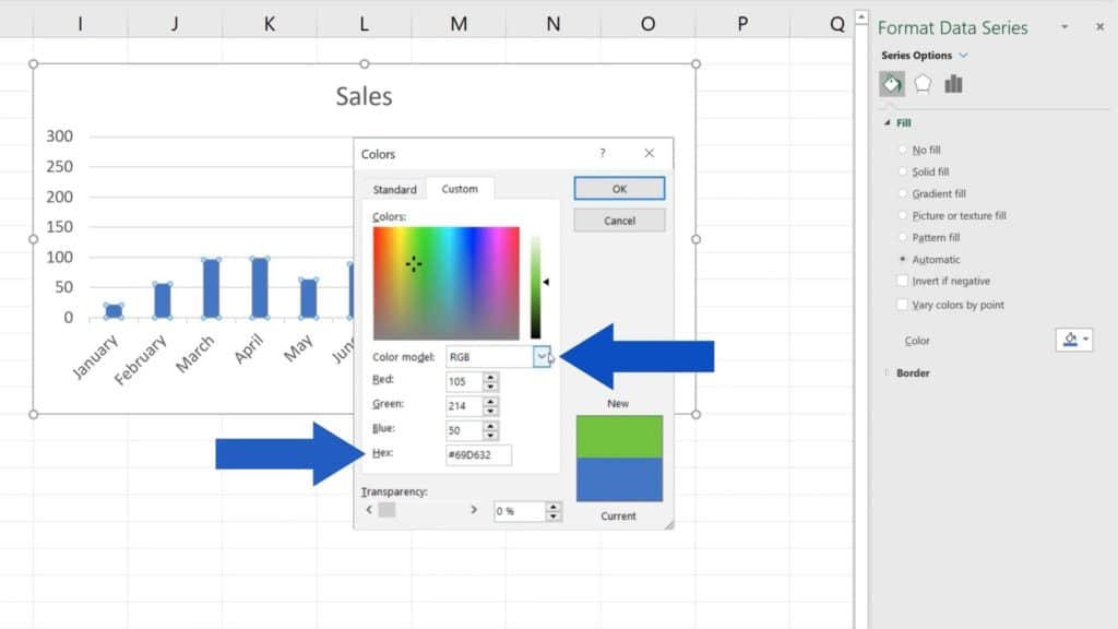
If this is not enough of a choice, you can use the option ‘More Colors’ at the bottom. Here you can mix any colour you need or you can define an exact colour using an RGB or a HEX code.
Let’s select this bright red and click on OK.
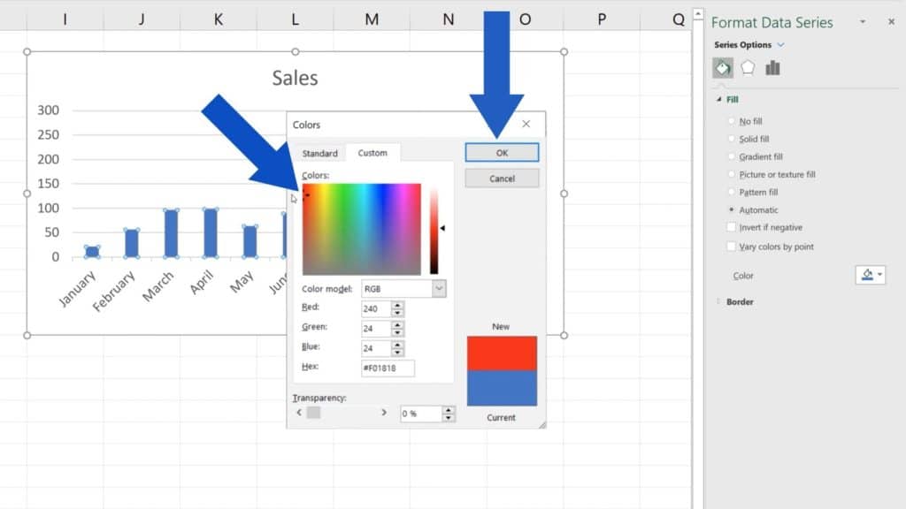
Excel will promptly change the bars colour to the one we’ve chosen.
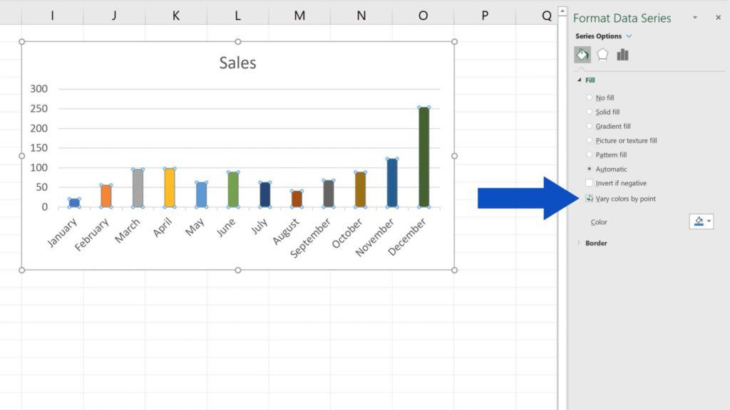
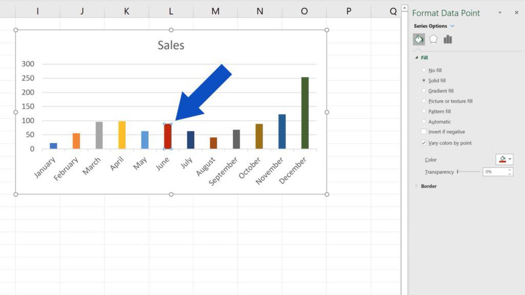
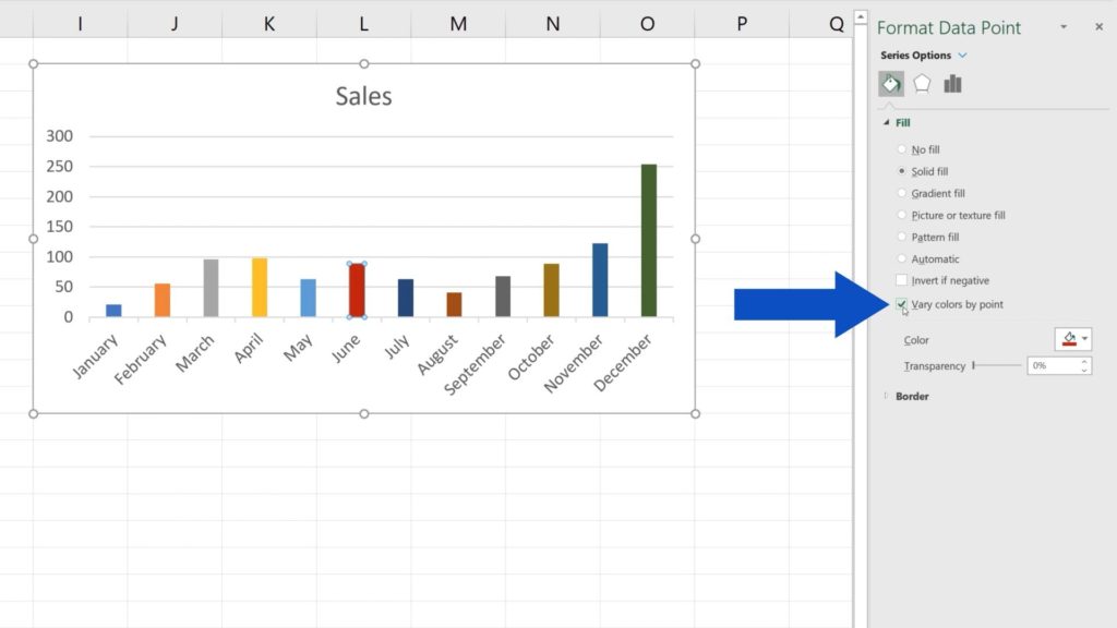
How to Use a Different Colour for Each Bar
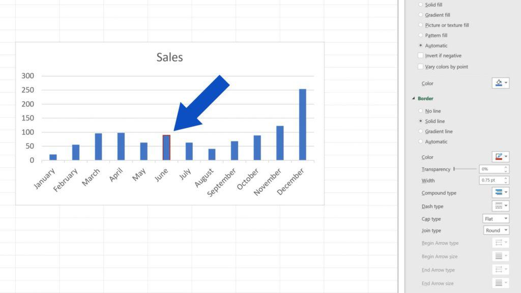
What’s amazing about this is that you’re not limited to use just one colour for all bars. To use a different colour for each bar, select the option ‘Vary colors by point’. Every bar in the chart now has its own colour fill and every single one can now be adjusted the way we saw a while ago.
Let’s click on the June bar, for example, and change the green to this dark red.
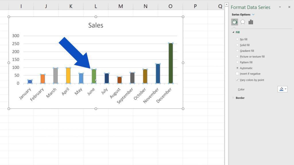
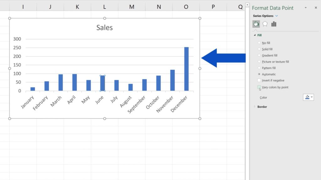
If you decide to return to only one colour for all the bars, simply unselect ‘Vary colors by point’ and that’s it! The chart’s back to one colour only!
And there’s one more thing worth knowing about.
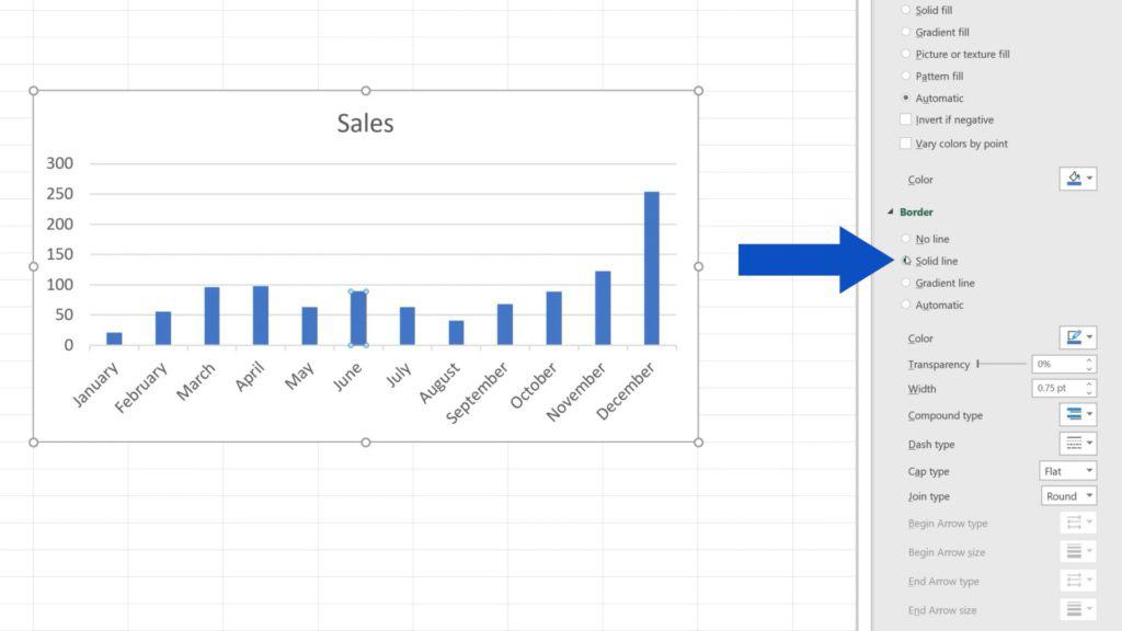
How to Adjust Borders of the Chart Bars
In terms of colours, you can easily adjust borders of the chart bars, too. Expand the ‘Border’ option and you’ll see another, very similar menu that applies to the borders of the bars.
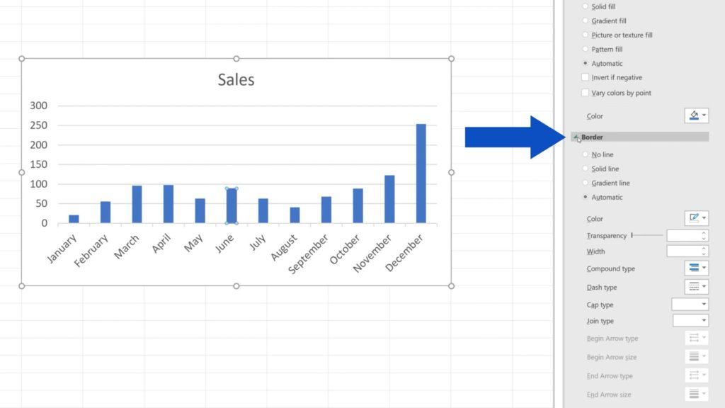
Let’s select ‘Solid line’ here and change the blue colour of the borders of the June bar to – let’s say – red.
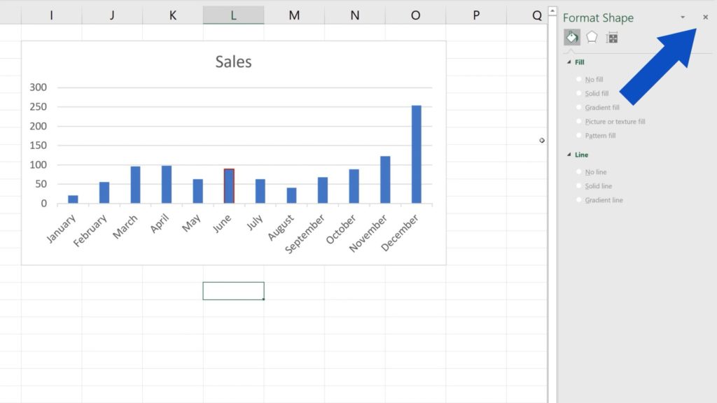
Here we go!
As soon as you’ve finished formatting the bar chart, simply close the pane by clicking on the X in the upper right corner.
There are a lot of great things you can do with your charts!
If you’re interested to see how you can format other elements in the chart, check out the links to more tutorials by EasyClick Academy! You’ll find them in the list below!
Don’t miss out a great opportunity to learn:
- How to Change Chart Style in Excel
- How to Add a Title to a Chart in Excel (In 3 Easy Clicks)
- How to Add Axis Titles in Excel
- How to Add a Trendline in Excel
If you found this tutorial helpful, give us a like and watch other video tutorials by EasyClick Academy. Learn how to use Excel in a quick and easy way!
Is this your first time on EasyClick? We’ll be more than happy to welcome you in our online community. Hit that Subscribe button and join the EasyClickers!
Thanks for watching and I’ll see you in the next tutorial!