
Change the format of a cell
You can apply formatting to an entire cell and to the data inside a cell—or a group of cells. One way to think of this is the cells are the frame of a picture and the picture inside the frame is the data.

Formal Cells
-
Select the cells.
-
Go to the ribbon to select changes as Bold, Font Color, or Font Size.
Apply Excel Styles
-
Select the cells.
-
Select Home > Cell Style and select a style.
Modify an Excel Style
-
Select the cells with the Excel Style.
-
Right-click the applied style in Home > Cell Styles.
-
Select Modify > Format to change what you want.
Need more help?
You can always ask an expert in the Excel Tech Community or get support in the Answers community.
See Also
Format text in cells
Format numbers
Format a date the way you want
Need more help?
Want more options?
Explore subscription benefits, browse training courses, learn how to secure your device, and more.
Communities help you ask and answer questions, give feedback, and hear from experts with rich knowledge.
When you fill out Excel worksheets with data, no one will succeed at once, everything is beautiful and correctly filled at the first attempt.
In the process of working with the program, you always need something: modify, edit, delete, copy or move. If the entered incorrect values in a cell, naturally, we want to correct or delete ones. But even such simple task can sometimes create difficulties.
How to set the cell format in Excel?
The contents of each Excel cell consist of three elements:
- The meaning: text, numbers, dates and times, logical content, functions and formulas.
- The formats: the type and color of the borders, the type and color of the fill, the way the values are displayed.
- Comments.
All these three elements are completely independent of each other. You can specify the format of the cell and do not write anything to it, or add a note in an empty and not formatted cell.
How to change the format of cells in Excel?
To change the format of the cells, you should call the corresponding dialog box with the CTRL + 1 (or CTRL + SHIFT + F) key or from the context menu after you right-click the «Cell Format» option.
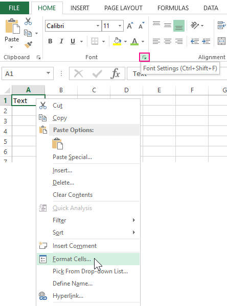
There are 6 tabs in this dialog box:
- A number. Here you specify the way the numeric values are displayed.
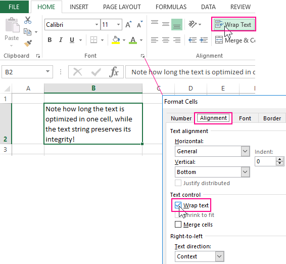
- The alignment. On this tab you can control the position of the text. And the text can be displayed vertically or diagonally from any angle. Also pay attention to the «Display» section. Very often, the function «Wrap Text» is used.
- Font. The specify the style design of fonts, the size and color of the text, plus the modes of modifications.
- The border. Here you define the styles and colors of the borders. The design of all tables is better done right here.
- The fill. The name of the bookmark speaks for itself. Available for formatting colors, patterns and methods of filling (for example, a gradient with a different direction of strokes).
- The protection. Here, the cell protection settings are set, that are activated only after the protection of the whole sheet.
If you did not get the desired result on the first attempt, call this dialog again to fix the cell format in Excel.
What formatting is applicable to cells in Excel?
Each cell always has some format. If there were no changes, then this is the «General» format. It is also a standard Excel format, in which:
- the numbers are aligned on the right side;
- the text is aligned on the left side;
- the font Calibri with the height of 11 points;
- the cell has no borders and background fill.
The Format Removal – is the changing to the standard «General» format (without borders and fills).
It is worth noting that the format of cells, unlike values, can not be deleted with the DELETE key.
To delete the format of cells, select ones and use the «Clear Formats» tool, which is located on the «HOME» tab in the «Editing» section.
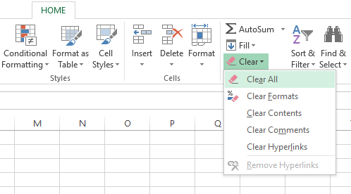
If you want to clear not only the format, but also the values, then select the «Clear All» option from the drop-down list of the tool (eraser).
As you can see, the eraser tool is functionally flexible and allows us to make a choice of what to delete in the cells:
- the content (same as the DELETE key);
- the formats;
- notes;
- the hyperlinks.
The option «Clear all» combines all these functions.
The deleting notes
Note, as well as formats, are not deleted from the cell by pressing the DELETE key. You can delete notes in two ways:
- The eraser tool: the option «Clear notes».
- Click on the cell with the note with the right mouse button, and from the appeared context menu select the option «Delete note».
The notation. The second way is more convenient. If you delete several notes at the same time, you must first select all of its cells.
![]()
Download Article
![]()
Download Article
Knowing how to format your spreadsheet in Excel, the cells in particular, can really help you improve not just the aesthetic perspective of your document, but also its effectiveness in providing relevant information to the viewers of the files. Each cell in Microsoft Excel can be modified and formatted to follow your specific preferences.
-

1
Open your Microsoft Excel. Click the “Start” button on the lower-left corner of your screen and select “All Programs” from the menu. Inside, you’ll find the “Microsoft Office” folder where Excel is listed. Click on Excel.
-
2
Select the specific cell or group of cells that you want to format. Highlight it using your mouse cursor.
Advertisement
-
3
Open the Format Cells window. Right-click on the cells you’ve selected and select “Format Cells” from the pop up menu to access the “Format Cells” window.
-
4
Set the desired formatting options you want for the cell. There are six formatting options that you can use to customize a cell or group of cells:
- Number – Defines the format of numerical data entered on the cells such as dates, currency, time, percentage, fraction and more.
- Alignment – Sets how the data will be visually aligned inside each cells (left, right or centered).
- Font – Sets all the options related to text fonts such as styles, sizes and colors.
- Border – Improves the visual appearance of each cell by adding definite lines (borders) around a cell or group of cells.
- Fill – Sets the background color and pattern formats of each cell on the spreadsheet.
- Protection – Adds security to cells and data contained inside it by hiding or locking the selected cells or group of cells.
-
5
Save. Click on the “OK” button at the lower right corner of the “Format Cells” window to save any changes you’ve made and apply the formats you’ve set to the selected cells.


Advertisement
Ask a Question
200 characters left
Include your email address to get a message when this question is answered.
Submit
Advertisement
-
Avoid using formats that are visually irritating such as fill colors that don’t compliment the colors of the fonts, or artistic font styles that are not appropriate for formal documents like the spreadsheet.
-
You can use this method to format cells of new files or existing spreadsheet documents you currently have.
-
When formatting cells in Excel, do it in groups (either by rows or columns) so that your spreadsheet will have a clean and uniform appearance.
Thanks for submitting a tip for review!
Advertisement
About This Article
Article SummaryX
To format a cell in Microsoft Excel, start by highlighting the specific cell you want to format. Then, right-click on the cell and click on «Format Cells.» Choose whatever formatting you want for the cell from the different options, then click «Okay.» That’s all there is to it! For a step-by-step walkthrough with pictures, check out the full article below!
Did this summary help you?
Thanks to all authors for creating a page that has been read 72,532 times.
Is this article up to date?
When working with data and formulas in Excel, one of the important points is the format of the cells. Data can be presented in completely different ways.
For example, the number 23 in a cell with a percentage format will be stored as 0.23 float, while in a cell with the numeric format as 23 integers. The number 45,678 when using commas to separate thousands, Excel will store as 45 thousand and 678, while in a cell with the data format, you will most likely see 1/21/2025 (see how to adjust the number of digits after the decimal point):

To apply the format to the selected cell or range of cells, do the following:
- Using the keyboard:
- On the Home tab, in the Number group, open the Number Format dropdown list:

From the Number Formats dropdown list:

- Choose one of the 11 common number formats (see below),
- Select the More Number formats… to create a custom format (see Custom cell format for more details):

- Do one of the following:
- Right-click on the selection and choose Format Cells… in the popup menu:

- On the Home tab, in the Number group, click the dialog box launcher:

In the Format Cells dialog box, on the Number tab, in the Category list:

- Choose one of the 11 predefined formats,
- Use the Custom format (see Custom cell format for more details).
- Right-click on the selection and choose Format Cells… in the popup menu:


- Using the mouse: Number-Formatting Keyboard Shortcuts:
Key Combination Formatting Applied Ctrl+Shift+~ General number format (that is, unformatted values) Ctrl+Shift+$ Currency format with two decimal places (negative numbers appear in parentheses) — see how to change the currency format Ctrl+Shift+% Percentage format, with no decimal places Ctrl+Shift+^ Scientific notation number format, with two decimal places Ctrl+Shift+# Date format with the day, month, and year — DD-MM-YYYY [email protected] Time format with the hour, minute, and AM or PM Ctrl+Shift+! Two decimal places, thousands separator, and a hyphen for negative values:

Note: The number format does not affect the value. It affects only the appearance. See also Different rounding effects in Excel.
Number formats
- General (used by default) displays numbers as integers or decimals and in scientific notation if the value is too wide to fit in the cell.
- Number allows to specify:
- the number of decimal places,
- whether to use a comma to separate thousands,
- how to display negative numbers — with a minus sign, in red, in parentheses, or in red and in parentheses:

- Currency allows to specify:
- the number of decimal places,
- whether to use a comma to separate thousands,
- a currency symbol,
- how to display negative numbers — with a minus sign, in red, in parentheses, or in red and in parentheses.
- Accounting differs from the Currency format in that the currency symbols always align vertically (see more about differences between currency and accounting formats).
- Date allows selecting one of several date formats.
- Time allows selecting one of several time formats.
- Percentage allows specifying the number of decimal places and always displays a percent sign.
- Fraction allows selecting from among nine fraction formats.
- Scientific displays numbers in exponential notation — with letter E or e: 2.00E+08 = 200,000,000; 1.02E+05 = 102,000.
You can choose the number of decimal places to display to the left of E. The second example can be read as «1.02 times 10 to the fifth.»
- Text allows specifying a value that causes Excel to treat it as text, even if it looks like a number.
This feature is useful for such items as serial numbers, credit card numbers, or document numbers.
- Special contains additional number formats.
In the U.S. version of Excel, the additional number formats are Zip Code, Zip Code + 4, Phone Number, and Social Security Number:

- Custom enables to define custom number formats – see Custom cell format for more details.


Note: If a cell displays a series of hashes such as #########, this usually means that the column width is not wide enough to display the value in the selected number format. To display the value correctly, change the column width (see How to change width of gridlines in Excel) or change the number format.
The series of hashes can also indicate a negative time value (see How to format negative timestamps) or an invalid date, such as a date before January 1, 1900.
See also this tip in French:
Comment changer le format de numéro facilement.
Microsoft Excel has many formats for entering content inside a cell. By default when you open a workbook, all cells are available in “General” format. Excel will accept text content inside cells without any errors. However, when you enter number inside a “General” formatted cell, you will see a validation error. Here are simple shortcuts to change cell format in Excel quickly.
Related: How to insert sigma or summation symbol in Excel?
Cell Validation Error
In the Excel worksheet, you need to look for tools in the ribbon and then format the menu according to the data you want to enter in the cells. Below is the screenshot of Excel in Office 365 version on Mac. You can change the format under “Home” tab by clicking on the format dropdown box.

You have to change the desired format before typing the content. Otherwise, Excel will show you error with a green mark on the top left corner within the cell. You can hover over the cell and click on the warning symbol to see more details. For example, when you type number inside a general cell and press enter, you will see “Number Stored As Text” warning.

Therefore, it is necessary to change the cell format before you enter the content inside a cell.
However, navigating through menu and changing the cell format is time consuming task. In order not to waste time, Excel provides some shortcut keys for changing cell format. You can find them below:
| Shortcut | Cell Format |
|---|---|
| Ctrl + Shift + ~ | General format |
| Ctrl + Shift + ! | Number format with two decimals and thousand separator |
| Ctrl + Shift + @ | Time format, you can set AM / PM |
| Ctrl + Shift + # | Date format, change the cell value to default date format |
| Ctrl + Shift + $ | Currency format, adds the default currency symbol to number with two decimal. Negative value will show with red color and inside brackets. |
| Ctrl + Shift + % | Percentage format |
| Ctrl + Shift + ^ | Scientific format |
Good part is these keyboard shortcuts for changing cell format will work both on Windows and Mac Excel version.
Example
Below is an example, how the cell value 123 will change when you apply these shortcuts to change the format:
| Value | Shortcut | Result | Format |
|---|---|---|---|
| 123 | Control + Shift + ~ | 123 | General |
| 123 | Control + Shift + ! | 123.00 | Number |
| 123 | Control + Shift + @ | 12:00 AM | Time |
| 123 | Control + Shift + # | 2-May-00 | Date |
| 123 | Control + Shift + $ | ¥123.00 | Currency |
| 123 | Control + Shift + % | 12300% | Percentage |
| 123 | Control + Shift + ^ | 1.23E+02 | Scientific |

2
Editing is common when we need to change things in any cell. So it is vital to practice the shortcut key for this particular task. Often, we may need to edit the cell’s content. Often, we may need to edit the formula or debug the formula, so the shortcut is very important. Furthermore, it is important to practice shortcut keys to cut the short time for specific tasks as a new learner. So let us start one of the keyboard shortcut keys to edit a cell in Excel. This article will show you the efficient editing techniques of the cells using shortcut keys.
Table of contents
- Excel Edit Cell Shortcut
- Editing Cells in Excel
- Edit Cell Using Excel Shortcut Key
- Tips for Editing Cells in Excel
- Things to Remember
- Recommended Articles
Editing Cells in Excel
In Excel, editing is possible at the cell level at a time. However, we can edit only one cell, so we usually write formulas, edit them, and make corrections to the formulas to debug any issues.
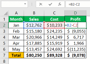
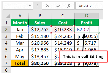
For example, let us look at the below data in Excel.

In column “D,” we have formulas. So, if we want to edit the formula, we can do it in two ways: manual and keyboard shortcut keyAn Excel shortcut is a technique of performing a manual task in a quicker way.read more. Both are simple and take an equal amount of time. So, let us look at them one by one in detail.
If we want to edit the cell D2 formula, we first need to select the cell for editing.

In the “Formula” bar, we can see the basic excel formulasThe term «basic excel formula» refers to the general functions used in Microsoft Excel to do simple calculations such as addition, average, and comparison. SUM, COUNT, COUNTA, COUNTBLANK, AVERAGE, MIN Excel, MAX Excel, LEN Excel, TRIM Excel, IF Excel are the top ten excel formulas and functions.read more. So to edit the formula, we can directly click on the “Formula” bar. It will show the result like this.

The moment we put our cursor (we can see the small blinking straight line) in the “Formula” bar. It has gone to editing mode. In the cell, we can see only the formula, not the result of the formula.
So, this is the way of editing the cells. We can edit cells and formulas by directly placing the cursor on the formula bar in Excel.
Another way of editing the cells, i.e. double-clicking on the cell. So, first, we need to select the cell that we wish to edit and then double-click on the cell. As a result, it will go to edit mode.
Since we double-clicked on the cell, it has gone to edit mode.
We can notice one more thing here: editing a blinking straight line appears itself in the cell rather than the formula cell, as in the previous example.
There is a way to identify the formula bar editing and in-cell editing, i.e.; it would be that editing mode wherever colored cell reference is highlighted.

Edit Cell Using Excel Shortcut Key
We can also use the keyboard shortcut keys to edit the Excel cells. For example, the shortcut key is “F2,” so pressing the F2 key will take us from the active cell to editing mode.

For example, suppose we want to edit cell D2. So, first, we need to press the F2 key by selecting the cell.

As we can see above, this works like in-cell editing, where a blinking straight line appears inside the cell rather than in the “Formula” bar. However, by changing default settings, we can make this change happen.
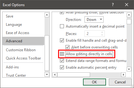
Follow the below steps to make the edit in the Excel “Formula” bar.
- We must first go to the “File” tab. Under this, go-to “Options.”

- Now, click on the “Advanced” tab.

- After that, uncheck the box “Allow editing directly in cells.”

If we press the “F2” key on the keyboard as the Excel shortcut key, the blinking straight line may go to the “Formula” bar instead of in-cell itself.


Tips for Editing Cells in Excel
An “F2” shortcut key can put the cell into editing mode. But, we are the ones who need to make the changes. For example, let us look at the below content.

We have a spelling mistake, “savvve” in this example, so we must press the “F2” key to edit the cell.

Upon pressing the “F2” key, the edit gets activated at the end of the cell value. So, now we need to travel to the left side. By pressing the left arrow key, we can move one character at a time. To move one word instead of one character, we must hold the “Ctrl” key and press the left arrow. It will jump to the next word.

Like this, we can use the keyboard shortcut keys to edit the Excel cell to the full extent.
Things to Remember
- By default, we can use the “F2” shortcut key for editing in the cell. But by changing the settings, we can make this happen at the “Formula” bar.
- Edit happens at the end of the cell’s value. We may go to the middle of the cell’s value by placing the cursor anywhere.
Recommended Articles
This article has been a guide to Excel shortcuts to edit the cell. Here, we discuss the different ways of editing the cells using shortcut keys and practical examples. You may learn more about Excel from the following articles: –
- Select Row Shortcut in Excel
- How to Write Formula in Excel?
- Percent Change in Excel
- Convert to Lower Case in Excel
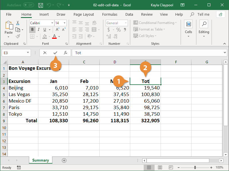
Cell data is the text or the numbers within a cell. It can be text you type in, numbers, or formulas. When you start creating a spreadsheet, one of the first steps is to enter data in the cells.
Enter Cell Data
- Click the blank cell where you want to add data.
You know the cell is active because a border appears around it.
- Type your data into the cell.
Notice that the text you type also appears in the Formula bar.
- Press Enter or click the Enter button.

Replace Cell Data
In addition to adding data in a blank cell, you can also type data into a cell that is already populated.
- Select the cell that contains the data you want to replace.
The old information is automatically selected.
- Enter the new information.
- Press Enter or click the Enter button.
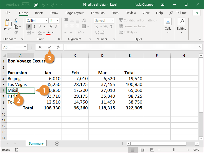
The new information is added in the old data’s place.
Delete Cell Data
If you want to remove the data all together, you can delete it.
- Select the cell that contains that data you want to delete.
- Press the Delete key on your keyboard.
The data is deleted from the selected cell.
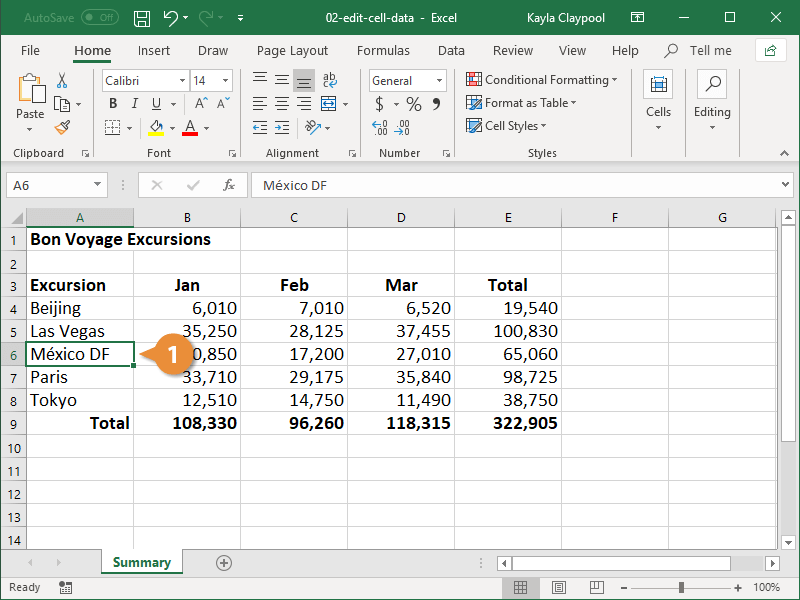
Edit Cell Data
In addition to replacing and deleting data, you can also make edits.
- Click the cell you want to edit.
- Click in the formula bar.
- Make your changes.
- Press Enter or click the Enter button.
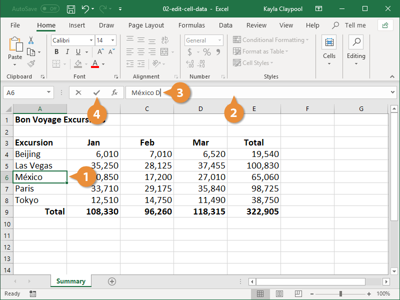
The cell is updated with the new text.

FREE Quick Reference
Click to Download
Free to distribute with our compliments; we hope you will consider our paid training.
Whether you are working on Microsoft Excel or other spreadsheet programs, the content will appear in a rectangular grid of cells. You will see that each cell has the same size in a row and column, that’s why you cannot change the cell’s size individually. Changing the size of a cell will directly affect other cells in the same row or column.
So, the thing is how to make cells bigger in Excel without interrupting other settings. To form bigger compound cells, merging adjacent cells will help, or else you may change the settings of rows and columns so that the content fits automatically.
How to Make Cells Bigger in Excel on a PC
Running Microsoft Excel on a PC, iPhone or Android seems different. However, with a PC, it works amazingly. On a PC, you will have an option to work on Excel along with other relevant apps such as Microsoft PowerPoint and Microsoft Word. No matter why you need to make cells bigger in Excel, the thing is you can simply make changes in the sheet individually to make cells bigger.
Let’s find out how you can do it:
- Choose the cell you need to resize and clear the adjacent cells from all directions. Now, you have to highlight the whole set. Most likely, you would need to move the data of those cells to other cells in the sheet.
- Hit the Home tab right from the file.

- Scroll down to the “Alignment” section and hit the down arrow placed next to the “Merge & Center” option.

- Choose this “Merge & Center” option.

- Now, you will see a bigger cell that is surrounded by all the normal size cells. It’s up to you how you will add content in this bigger cell.
How to Make Cells Bigger in Excel Using Wrap Text Option
Here comes another great method that helps in making cells bigger individually. Let’s dig out how you can do it:
- You will have to choose the first cell of the Email ID column and hit the Home tab; after that click on the “Wrap Text” option.

- Later on, you will see the first cell is bigger and the content fits in.
- Once the content fits in, you have to copy the format and click on the Home tab > Format Painter option.
- Drag down the indicated sign.

- Doing this will help you fit the entire content in the bigger cells.

How to Make Cells Bigger in Excel while Fixing Column Width with a Mouse Click
- Choose the Email ID column and drag down the indicated sign to the right side, so that it fits in the Email Ids cells.
- Besides, you can even double-click on this sign.

Following these steps will ultimately give you desired results.

How to Make Cells Bigger in Excel while Fixing Column Width using Shortcut Trick
- Choose the column from which you need to change the size of the cells. Press ALT + H, O, I. ALT + H will open up the Home tab, O opens up the Format Group, and I choose the Autofit Column Width.

- This will end up fitting the content in a bigger cell by default.

How to Make Cells Bigger in Excel while Fixing Column Width using Format Option
- Choose the Email ID column and follow this sequence of operations: Home tab > Cells Group > Format > AutoFit Column Width

Following this step will fit your content automatically in a bigger cell.

How to Make Cells Bigger in Excel while Fixing Row Height using Format Option
- First of all, you need to choose the group of rows from which you want to make cells bigger. Here in this example, you will see Row 4 to Row 11 are highlighted. Follow the sequence of operations as; Home tab > Cells Group > Format > Row Height

- A dialog box “Row Height” will pop up and you need to enter the Row height as per your needs. In this example, the row height is 48 points.

- The Row heights will get bigger and later on, you will have to choose the Email Id column while following this sequence: Home tab > Wrap Text

- Now, the text will fit in the cells perfectly.

How to Make Cells Bigger in Excel on an iPhone
While using an iPhone typically restricts you from multiple apps and functions. As in Microsoft Excel, you can merge cells easily to make one bigger cell on an iPhone.
Let’s see how you can execute this operation:
- Open the Excel file and choose the cell you need to resize. Clear the cells from all directions.

- Click on the original cell. Now, you will see the cell is highlighted in blue. Apart from that, you will also see a blue dot in two corners (top left and bottom right) of the cell.

- Dragging those blue dots will help you choose all the cells that needed to merge.

- Right at the bottom of the screen, you will find the option “Merge”, click on it.

- Right after clicking on it, you will see a bigger cell that can fit the data you wanted to enter.

Dragging Column or Row to Resize the Cell
- On the right side of the column, try moving the cursor over the edge line. Continue doing this until you see an arrow with a double line on the edge line. This arrow helps in maximizing the column width or row.
- Drag the column or row right in the direction you need to increase it. For instance right or left, top or bottom
- Release the mouse and the size will set up automatically. Right after finishing this step, you will get one bigger cell in the row or column.

Make Space for Anything You Need
Using Microsoft will never make you upset as you can fully customize your files. This app has a bunch of features to manipulate the settings as per your needs. Changing the cell size in the range of other standard-sized cells needs you to use the “Merge & Center” feature. It does not matter which platform you are using to change the cell size, you can quickly make cells bigger in Excel right after following some useful steps
Upon launching Microsoft Excel, an exactly-formatted spreadsheet grid is presented for you to start filling in. Every cell in a default Microsoft Excel spreadsheet is exactly the same size as all of the other cells within the spreadsheet, comprising the rows and columns on the screen. The spreadsheet isn’t locked, though. You can change cell width and height to put emphasis on certain information, make font sizes fit or to add white space to your spreadsheet. Excel doesn’t permit solo cell changes; size works on a row or column buddy system.
-
Open Microsoft Excel. To change cell size on an existing spreadsheet, click the “File” tab. Click “Open.” Navigate to the spreadsheet to change and double-click the file name.
-
Click into the cell you want to change. Note the highlighted column letter at the top of the screen and the row number on the left side of the screen.
-
Click the small line to the right of the column letter. For example, if the cell you want to change is in column D, click the small line between the D and E columns.
-
Drag the line to the right. This increases the width of the cell and all other cells in that column. Drag the line to the left to reduce the width of the cell.
-
Click the small line between the row numbers the cell is in. For example, if the cell you want to change is in row 4, click the line between rows 4 and 5.
-
Drag the line down the spreadsheet. This increases the height of the cell and all other cells in that row. Drag the line up, closer to row 3, to reduce the height of the cell.
Cells in Microsoft Excel 2010 have a default size of 8.43 characters wide by 15 points high. This size is ideal for many situations, but you will eventually encounter a piece of information that will not fit within these default parameters. Fortunately you can choose to make any cell either smaller or larger to accommodate the information that you are inputting into the cell. Additionally, there are several different methods that you can utilize to change the size of a cell in Microsoft Excel 2010, so you can experiment with the different available methods to determine which one is correct for your needs.
Check out our tutorial on how to expand all rows in Excel and learn about a quick and easy way to resize a lot of cells at once.
The first thing to realize before you start changing your Excel cell sizes is that when you are changing the width or height of a particular cell, you are adjusting that value for every other cell in the row or column. Excel will not allow you to change the size of a single cell.
Begin the process by double-clicking the Excel file that contains the cells that you want to resize.
Locate the cell that you want to adjust, then right click the column heading at the top of that cell’s column. The column heading is the letter above the spreadsheet.

Click the Column Width option, then enter a value into the field. You can enter any value into this field up to 255, but bear in mind that the default value is 8.43, so adjust accordingly. Once you have entered a new value, click OK.
Now that we have changed the width of the column, we are going to perform a very similar action to change the height. Right-click the row heading, which is the number at the far-left side of the spreadsheet, then click the Row Height option.

Type your desired row height value into the field (any value up to 409 will work) then click the OK button.
Do you often need to adjust your column width and want to use a shortcut? This Excel auto adjust column width shortcut method might be the answer you need.
While this method will work if you can accurately guess the cell width and height that you need, it could prove to be difficult if you do not know an approximate value. Luckily Excel 2010 also includes another option that will automatically resize your row or column for you, based upon the largest cell value in your selected row or column.
You can utilize this method by placing your mouse cursor on the line that separates your column or row heading from the one either to the right of or below it. For example, in the image below, I have placed my cursor on the line between columns B and C, because I want to automatically resize column B.

Double-click this line to have Excel automatically adjust the size of your row or column.
Note that both of these methods will work if you want to resize multiple rows or columns at once, too. Simply hold down the Ctrl or Select key on your keyboard to select all of the rows or columns that you want to resize, then use the Row Height, Column Width or double-click method to adjust the size values of the selected cells.
Our guide on how to autofit all columns in Excel can show you a simple way to fix the width of your spreadsheet columns.

Matthew Burleigh has been writing tech tutorials since 2008. His writing has appeared on dozens of different websites and been read over 50 million times.
After receiving his Bachelor’s and Master’s degrees in Computer Science he spent several years working in IT management for small businesses. However, he now works full time writing content online and creating websites.
His main writing topics include iPhones, Microsoft Office, Google Apps, Android, and Photoshop, but he has also written about many other tech topics as well.
Read his full bio here.