
Contents
- 1 How do I add categories to a drop down list in Excel?
- 2 How do I add categories and subcategories in Excel?
- 3 How do I create a conditional list in Excel?
- 4 How do I create categories in sheets?
- 5 How do you add a category to a label in Excel?
- 6 How do you create a hierarchy in Excel?
- 7 How do I create a dependent list in Excel?
- 8 How do I create a dynamic dependent list in Excel?
- 9 How do I create a sub category in Google Sheets?
- 10 How do I add a category in budget numbers?
- 11 How do you add multiple axis titles in Excel?
- 12 How do I create a multi axis chart in Excel?
- 13 How do I add a category and percentage data label in Excel?
- 14 How do I add category labels to a pie chart in Excel?
- 15 How do I create a one variable data table in Excel?
- 16 Where is the hierarchy button in Excel?
- 17 How do you create a hierarchy?
- 18 What is hierarchy in Excel?
- 19 How do I create a multi column Data Validation list in Excel?
- 20 What is an Xlookup in Excel?
How do I add categories to a drop down list in Excel?
Create a drop-down list
- Select the cells that you want to contain the lists.
- On the ribbon, click DATA > Data Validation.
- In the dialog, set Allow to List.
- Click in Source, type the text or numbers (separated by commas, for a comma-delimited list) that you want in your drop-down list, and click OK.
How do I add categories and subcategories in Excel?
Creating Subcategory in Drop Down List in Excel
- Enter the main category in a cell.
- In the cells below it, enter a couple of space characters and then enter the subcategory name.
- Use these cells as the source while creating a drop-down list.
How do I create a conditional list in Excel?
Dependent Drop-down Lists
- On the second sheet, create the following named ranges. Name. Range Address.
- On the first sheet, select cell B1.
- On the Data tab, in the Data Tools group, click Data Validation. The ‘Data Validation’ dialog box appears.
- In the Allow box, click List.
- Click in the Source box and type =Food. Result:
How do I create categories in sheets?
Create a drop-down list
- Open a spreadsheet in Google Sheets.
- Select the cell or cells where you want to create a drop-down list.
- Click Data.
- Next to “Criteria,” choose an option:
- The cells will have a Down arrow.
- If you enter data in a cell that doesn’t match an item on the list, you’ll see a warning.
- Click Save.
How do you add a category to a label in Excel?
Add data labels
Click the chart, and then click the Chart Design tab. Click Add Chart Element and select Data Labels, and then select a location for the data label option. Note: The options will differ depending on your chart type. If you want to show your data label inside a text bubble shape, click Data Callout.
How do you create a hierarchy in Excel?
Follow these steps:
- Open the Power Pivot window.
- Click Home > View > Diagram View.
- In Diagram View, select one or more columns in the same table that you want to place in a hierarchy.
- Right-click one of the columns you’ve chosen.
- Click Create Hierarchy to create a parent hierarchy level at the bottom of the table.
How do I create a dependent list in Excel?
Creating a Dependent Drop Down List in Excel
- Select the cell where you want the first (main) drop down list.
- Go to Data –> Data Validation.
- In the data validation dialog box, within the settings tab, select List.
- In Source field, specify the range that contains the items that are to be shown in the first drop down list.
How do I create a dynamic dependent list in Excel?
To make your primary drop-down list, configure an Excel Data Validation rule in this way:
- Select a cell in which you want the dropdown to appear (D3 in our case).
- On the Data tab, in the Data Tools group, click Data Validation.
- In the Data Validation dialog box, do the following: Under Allow, select List.
How do I create a sub category in Google Sheets?
Choose to group by “Category” for the columns selection. Add a second field to the columns selection and choose “subcategory.” Choose “Amount” for the “Values” field. Finally, add a filter to the pivot table for “Category” and choose only the “Food” category.
How do I add a category in budget numbers?
Select the table, click or tap the Organize button , then click or tap Categories. Click or tap Add a Category, then choose a column for the new subcategory you want to create. You can reorganize categories and subcategories in a table after you’ve added them.
How do you add multiple axis titles in Excel?
Click the chart, and then click the Chart Layout tab. Under Labels, click Axis Titles, point to the axis that you want to add titles to, and then click the option that you want. Select the text in the Axis Title box, and then type an axis title.
How do I create a multi axis chart in Excel?
Add or remove a secondary axis in a chart in Excel
- Select a chart to open Chart Tools.
- Select Design > Change Chart Type.
- Select Combo > Cluster Column – Line on Secondary Axis.
- Select Secondary Axis for the data series you want to show.
- Select the drop-down arrow and choose Line.
- Select OK.
How do I add a category and percentage data label in Excel?
To format data labels, select your chart, and then in the Chart Design tab, click Add Chart Element > Data Labels > More Data Label Options. Click Label Options and under Label Contains, pick the options you want.
How do I add category labels to a pie chart in Excel?
To add data labels to a pie chart:
- Select the plot area of the pie chart.
- Right-click the chart.
- Select Add Data Labels.
- Select Add Data Labels. In this example, the sales for each cookie is added to the slices of the pie chart.
How do I create a one variable data table in Excel?
To create a one variable data table, execute the following steps.
- Select cell B12 and type =D10 (refer to the total profit cell).
- Type the different percentages in column A.
- Select the range A12:B17.
- On the Data tab, in the Forecast group, click What-If Analysis.
- Click Data Table.
Where is the hierarchy button in Excel?
You can add a hierarchy chart to any Excel workbook regardless of its contents. Click on the Insert tab. This button is located on the navigation bar at the top your screen next to other options including Home, Formulas, and Review.
How do you create a hierarchy?
Create a hierarchy
- On the Insert tab, in the Illustrations group, click SmartArt.
- In the Choose a SmartArt Graphic gallery, click Hierarchy, and then double-click a hierarchy layout (such as Horizontal Hierarchy).
- To enter your text, do one of the following: Click [Text] in the Text pane, and then type your text.
What is hierarchy in Excel?
Advertisements. A hierarchy in Data Model is a list of nested columns in a data table that are considered as a single item when used in a Power PivotTable. For example, if you have the columns − Country, State, City in a data table, a hierarchy can be defined to combine the three columns into one field.
How do I create a multi column Data Validation list in Excel?
Excel 2007 and above
- Data tab / Data Validation module.
- In the name text box : name the range as List.
- Create a list of validations in E3 (Data/Validation, in Allow: select “List” in Source: type =List)
- Open the Name manager: Formula tab/set name/Name Manager, select the name of the range (List)
What is an Xlookup in Excel?
Use the XLOOKUP function to find things in a table or range by row.With XLOOKUP, you can look in one column for a search term, and return a result from the same row in another column, regardless of which side the return column is on.
Содержание
- How to Create Multi-Category Charts in Excel?
- Table :
- Implementation :
- How To Add Categories In Excel?
- How do I add categories to a drop down list in Excel?
- How do I add categories and subcategories in Excel?
- How do I create a conditional list in Excel?
- How do I create categories in sheets?
- How do you add a category to a label in Excel?
- How do you create a hierarchy in Excel?
- How do I create a dependent list in Excel?
- How do I create a dynamic dependent list in Excel?
- How do I create a sub category in Google Sheets?
- How do I add a category in budget numbers?
- How do you add multiple axis titles in Excel?
- How do I create a multi axis chart in Excel?
- How do I add a category and percentage data label in Excel?
- How do I add category labels to a pie chart in Excel?
- How do I create a one variable data table in Excel?
- Where is the hierarchy button in Excel?
- How do you create a hierarchy?
- What is hierarchy in Excel?
- How do I create a multi column Data Validation list in Excel?
- What Is A Category Label In Excel?
- How do you use category labels in Excel?
- How do you add a category to a graph in Excel?
- How do I add category labels to a pie chart in Excel?
- How do I change the axis category in Excel?
- What are data labels?
- How do I add a label to a cell in Excel?
- How do you category data in Excel?
- How do I create a category in spreadsheet?
- How do you categorize data in Excel?
- What are data labels on a pie chart?
- How do you label a graph?
- How do you label Axis in Excel for Mac?
- What are axis labels on a graph?
- How do I label something in Excel?
- What are labels and values in Excel?
- How do you categorize data?
- How do you classify text in Excel?
- How do I select all data labels in Excel?
How to Create Multi-Category Charts in Excel?
The multi-category chart is used when we handle data sets that have the main category followed by a subcategory. For example: “Fruits” is a main category and bananas, apples, grapes are subcategories under fruits. These charts help to infer data when we deal with dynamic categories of data sets. By using a single chart we can analyze various subcategories of data.
In this article, we will see how to create a multi-category chart in Excel using a suitable example shown below :
Example: Consider the employees from our organization working in various departments. The main categories under departments are “Marketing”, “Sales”, “IT”. Now under every department, there are multiple employees which is a subcategory.
Now, we would like to create a Multi-Category chart having the age details of employees from multiple departments. Consider the table shown below :
Table :
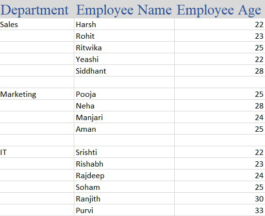
Employee Details Table
Implementation :
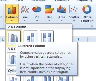
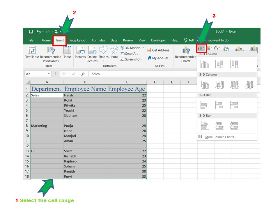
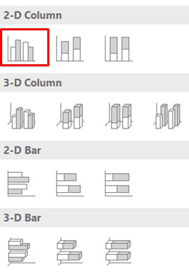
Step 1: Insert the data into the cells in Excel. Now select all the data by dragging and then go to “Insert” and select “Insert Column or Bar Chart”. A pop-down menu having 2-D and 3-D bars will occur and select “vertical bar” from it.
Bar Chart Insertion
Multi-Category Chart
An important thing to note is that sometimes few subcategory data may be missing in the chart after insertion. It is not an error and just by increasing the size of the chart the data will be shown.
The Multi-category chart is ready. Now we can perform various modifications to it to make the chart more insightful by adding titles, changing the width and gap, assigning different colors to different sub-categories.
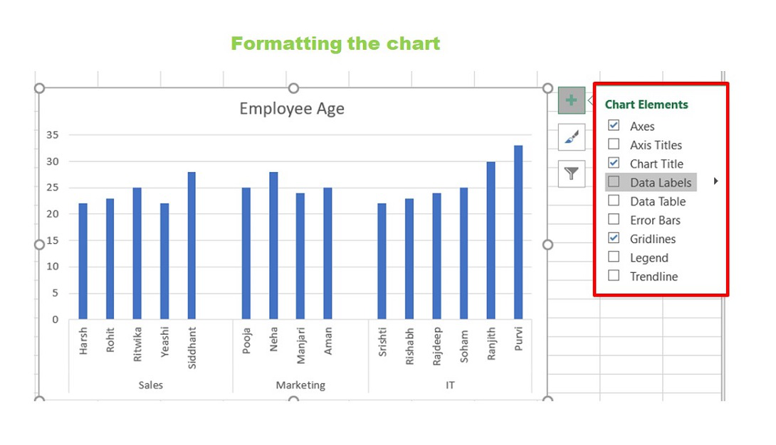
Step 2: For formatting, select the chart and use the “+” button beside it to add Title, Data labels, Axes Titles, and others or right-click and then select Format option.
- Adding Title: Check the “Chart Title” box from the Chart Elements pop down and add a suitable title.
- Adding data labels: Check the “Data Labels” from the Chart Elements pop down.
Data Labels
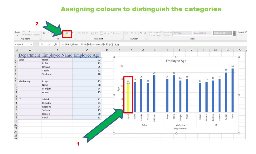
- Assigning a color to bars: Select the individual bar and add colors as shown below:
- Gap Width: Assign a suitable gap width as per requirements. Select all the bars, right-click on it and select “Format Data Series.”
Gap width
- Formatting Axis: Select the chart and then click on the “+” button and under “Axes” select “More Options”. Another way is to select the axis in the chart and then right-click and click on “Format Axis”.
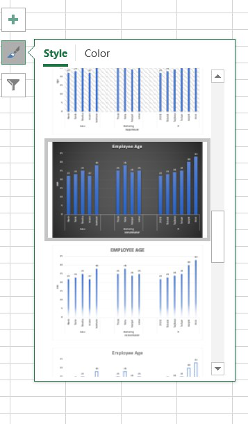
- Changing the chart style: Click on the Chart Styles beside the chart and select a suitable chart style.
Final Multi-Category Chart
- Changing the Chart Type: Suppose now we want the above chart in the form of horizontal bars.
Finally, Click on OK.
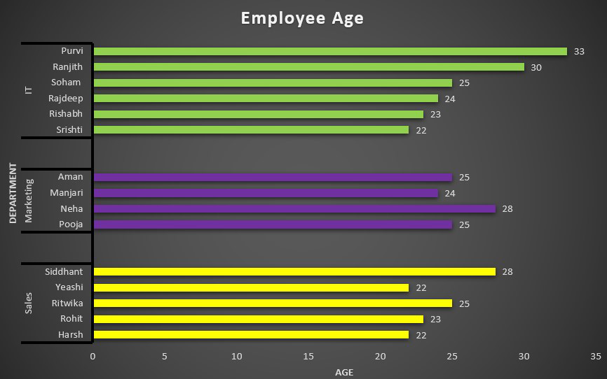
Final Horizontal Multi-Category chart
Источник
How To Add Categories In Excel?
How do I add categories to a drop down list in Excel?
Create a drop-down list
- Select the cells that you want to contain the lists.
- On the ribbon, click DATA > Data Validation.
- In the dialog, set Allow to List.
- Click in Source, type the text or numbers (separated by commas, for a comma-delimited list) that you want in your drop-down list, and click OK.
How do I add categories and subcategories in Excel?
Creating Subcategory in Drop Down List in Excel
- Enter the main category in a cell.
- In the cells below it, enter a couple of space characters and then enter the subcategory name.
- Use these cells as the source while creating a drop-down list.
How do I create a conditional list in Excel?
Dependent Drop-down Lists
- On the second sheet, create the following named ranges. Name. Range Address.
- On the first sheet, select cell B1.
- On the Data tab, in the Data Tools group, click Data Validation. The ‘Data Validation’ dialog box appears.
- In the Allow box, click List.
- Click in the Source box and type =Food. Result:
How do I create categories in sheets?
Create a drop-down list
- Open a spreadsheet in Google Sheets.
- Select the cell or cells where you want to create a drop-down list.
- Click Data.
- Next to “Criteria,” choose an option:
- The cells will have a Down arrow.
- If you enter data in a cell that doesn’t match an item on the list, you’ll see a warning.
- Click Save.
How do you add a category to a label in Excel?
Add data labels
Click the chart, and then click the Chart Design tab. Click Add Chart Element and select Data Labels, and then select a location for the data label option. Note: The options will differ depending on your chart type. If you want to show your data label inside a text bubble shape, click Data Callout.
How do you create a hierarchy in Excel?
Follow these steps:
- Open the Power Pivot window.
- Click Home > View > Diagram View.
- In Diagram View, select one or more columns in the same table that you want to place in a hierarchy.
- Right-click one of the columns you’ve chosen.
- Click Create Hierarchy to create a parent hierarchy level at the bottom of the table.
How do I create a dependent list in Excel?
Creating a Dependent Drop Down List in Excel
- Select the cell where you want the first (main) drop down list.
- Go to Data –> Data Validation.
- In the data validation dialog box, within the settings tab, select List.
- In Source field, specify the range that contains the items that are to be shown in the first drop down list.
How do I create a dynamic dependent list in Excel?
To make your primary drop-down list, configure an Excel Data Validation rule in this way:
- Select a cell in which you want the dropdown to appear (D3 in our case).
- On the Data tab, in the Data Tools group, click Data Validation.
- In the Data Validation dialog box, do the following: Under Allow, select List.
How do I create a sub category in Google Sheets?
Choose to group by “Category” for the columns selection. Add a second field to the columns selection and choose “subcategory.” Choose “Amount” for the “Values” field. Finally, add a filter to the pivot table for “Category” and choose only the “Food” category.
How do I add a category in budget numbers?
Select the table, click or tap the Organize button , then click or tap Categories. Click or tap Add a Category, then choose a column for the new subcategory you want to create. You can reorganize categories and subcategories in a table after you’ve added them.
How do you add multiple axis titles in Excel?
Click the chart, and then click the Chart Layout tab. Under Labels, click Axis Titles, point to the axis that you want to add titles to, and then click the option that you want. Select the text in the Axis Title box, and then type an axis title.
How do I create a multi axis chart in Excel?
Add or remove a secondary axis in a chart in Excel
- Select a chart to open Chart Tools.
- Select Design > Change Chart Type.
- Select Combo > Cluster Column – Line on Secondary Axis.
- Select Secondary Axis for the data series you want to show.
- Select the drop-down arrow and choose Line.
- Select OK.
How do I add a category and percentage data label in Excel?
To format data labels, select your chart, and then in the Chart Design tab, click Add Chart Element > Data Labels > More Data Label Options. Click Label Options and under Label Contains, pick the options you want.
How do I add category labels to a pie chart in Excel?
To add data labels to a pie chart:
- Select the plot area of the pie chart.
- Right-click the chart.
- Select Add Data Labels.
- Select Add Data Labels. In this example, the sales for each cookie is added to the slices of the pie chart.
How do I create a one variable data table in Excel?
To create a one variable data table, execute the following steps.
- Select cell B12 and type =D10 (refer to the total profit cell).
- Type the different percentages in column A.
- Select the range A12:B17.
- On the Data tab, in the Forecast group, click What-If Analysis.
- Click Data Table.
Where is the hierarchy button in Excel?
You can add a hierarchy chart to any Excel workbook regardless of its contents. Click on the Insert tab. This button is located on the navigation bar at the top your screen next to other options including Home, Formulas, and Review.
How do you create a hierarchy?
Create a hierarchy
- On the Insert tab, in the Illustrations group, click SmartArt.
- In the Choose a SmartArt Graphic gallery, click Hierarchy, and then double-click a hierarchy layout (such as Horizontal Hierarchy).
- To enter your text, do one of the following: Click [Text] in the Text pane, and then type your text.
What is hierarchy in Excel?
Advertisements. A hierarchy in Data Model is a list of nested columns in a data table that are considered as a single item when used in a Power PivotTable. For example, if you have the columns − Country, State, City in a data table, a hierarchy can be defined to combine the three columns into one field.
How do I create a multi column Data Validation list in Excel?
Excel 2007 and above
- Data tab / Data Validation module.
- In the name text box : name the range as List.
- Create a list of validations in E3 (Data/Validation, in Allow: select “List” in Source: type =List)
- Open the Name manager: Formula tab/set name/Name Manager, select the name of the range (List)
Источник
What Is A Category Label In Excel?
In charts, axis labels are shown below the horizontal (also known as category) axis, next to the vertical (also known as value) axis, and, in a 3-D chart, next to the depth axis. The chart uses text from your source data for axis labels. To change the label, you can change the text in the source data.
How do you use category labels in Excel?
From the Design tab, Data group, select Select Data. In the dialog box under Horizontal (Category) Axis Labels, click Edit. In the Axis label range enter the cell references for the x-axis or use the mouse to select the range, click OK. Click OK.
How do you add a category to a graph in Excel?
How to Create Multi-category Charts in Excel
- Select the entire data set.
- Go to Insert –> Column –> 2-D Column –> Clustered Column. You can also use the keyboard shortcut Alt + F1 to create a column chart from data.
How do I add category labels to a pie chart in Excel?
To add data labels to a pie chart:
- Select the plot area of the pie chart.
- Right-click the chart.
- Select Add Data Labels.
- Select Add Data Labels. In this example, the sales for each cookie is added to the slices of the pie chart.
How do I change the axis category in Excel?
In a chart, click the category axis that you want to change, or do the following to select the axis from a list of chart elements:
- Click anywhere in the chart.
- On the Format tab, in the Current Selection group, click the arrow next to the Chart Elements box, and then click Horizontal (Category) Axis.
What are data labels?
Data labels are text elements that describe individual data points. Displaying data labels. You may display data labels for all data points in the chart, for all data points in a particular series, or for individual data points. For information, see Displaying Data Labels. Data label text.
How do I add a label to a cell in Excel?
Add a label or text box to a worksheet
- Click Developer, click Insert, and then click Label .
- Click the worksheet location where you want the upper-left corner of the label to appear.
- To specify the control properties, right-click the control, and then click Format Control.
How do you category data in Excel?
- Highlight the rows and/or columns you want sorted.
- Navigate to ‘Data’ along the top and select ‘Sort.
- If sorting by column, select the column you want to order your sheet by.
- If sorting by row, click ‘Options’ and select ‘Sort left to right.
- Choose what you’d like sorted.
- Choose how you’d like to order your sheet.
How do I create a category in spreadsheet?
First, insert a column into your spreadsheet between your Items list and Estimated Cost. Then, label the column Category. To make categorizing expenses easy and quick, use data validation to create a drop-down menu of categories to choose from right in your budget sheet.
How do you categorize data in Excel?
Sorting levels
- Select a cell in the column you want to sort by.
- Click the Data tab, then select the Sort command.
- The Sort dialog box will appear.
- Click Add Level to add another column to sort by.
- Select the next column you want to sort by, then click OK.
- The worksheet will be sorted according to the selected order.
What are data labels on a pie chart?
Pie chart data labels can be used to display the values of the slices or to show the series names without using a legend.
How do you label a graph?
The proper form for a graph title is “y-axis variable vs. x-axis variable.” For example, if you were comparing the the amount of fertilizer to how much a plant grew, the amount of fertilizer would be the independent, or x-axis variable and the growth would be the dependent, or y-axis variable.
How do you label Axis in Excel for Mac?
Adding an Axis Title
- Click the chart.
- Click Toolbox. The Formatting Palette appears.
- From the Formatting Palette, click Chart Options.
- From the Titles pull-down menu, select the desired axis.
- From the Click here to add title text box, type the desired axis title.
- (Optional) To reposition your axis title,
What are axis labels on a graph?
Axis labels are words or numbers that mark the different portions of the axis. Value axis labels are computed based on the data displayed in the chart. Category axis labels are taken from the category headings entered in the chart’s data range. Axis titles are words or phrases that describe the entire axis.
How do I label something in Excel?
Click the chart, and then click the Chart Design tab. Click Add Chart Element and select Data Labels, and then select a location for the data label option. Note: The options will differ depending on your chart type. If you want to show your data label inside a text bubble shape, click Data Callout.
What are labels and values in Excel?
Entering data into a spreadsheet is just like typing in a word processing program, but you have to first click the cell in which you want the data to be placed before typing the data. All words describing the values (numbers) are called labels. The numbers, which can later be used in formulas, are called values.
How do you categorize data?
Categorizing Data
- Determine whether a value calculated from a group is a statistic or a parameter.
- Identify the difference between a census and a sample.
- Identify the population of a study.
- Determine whether a measurement is categorical or qualitative.
How do you classify text in Excel?
You will see that after opening the spreadsheet with your data in Excel, you will be able to analyze them in just a few clicks.
- Step 1: open the Text Classification interface.
- Step 2: select the data to analyze.
- Step 3: configure the analysis.
- Step 4: analyze the results.
How do I select all data labels in Excel?
Can you select all data labels at once, and change them all at once.
The Tab key will move among chart elements.
- Click on a chart column or bar.
- Click again so only 1 is selected.
- Press the Tab key. Each column or bar in the series is selected in turn, then it moves to selecting each data label in the series.
Источник
It is possible to create a multi-category chart in Excel (as shown below).
The trick is to arrange the data in a certain way, that makes Excel interpret as having multiple categories.
Suppose I have the data for the monthly expenses I make on the food items (as listed below). The idea to create a chart for these items, and also categorize these as Fruits, Vegetables, and Packaged Food.
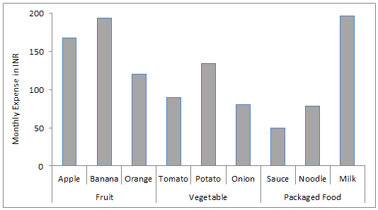
This is no rocket science. All you need is to arrange your data as shown below. Note that I have just added the overall category name (such as Fruit, Vegetable..) in a column on the left of the category name (apple, banana, orange..)

If you have the data arranged, as shown above, here are the steps to make this chart:
- Select the entire data set.
- Go to Insert –> Column –> 2-D Column –> Clustered Column.
- You can also use the keyboard shortcut Alt + F1 to create a column chart from data.
- That’s it!! You will have your chart. Format it the way you want.
Related Tutorials:
- Creating combination charts in Excel.
Multi-category chart or multi-level category chart is a chart type that has both main category and subcategory labels. This type of chart is useful when you have figures for items that belong to different categories.

Note: This tutorial uses Excel 2013. In other Excel versions, there may be some slight differences in the described steps.
Watch the video below to see how to create a multi-category chart in Excel. If you prefer written instructions, then continue reading.
Creating a multi-category chart in Excel
To create a multi-category chart in Excel, take the following steps:
1. Arrange the data in the following way: Enter main category names in the first column, subcategory names in the second column and the figure for each subcategory in the third column in the format shown below. For the purpose of this tutorial, suppose you have sales figures for different products of an online store for a month. The store’s products fall under 3 main categories: clothing, shoes and accessories.

2. Select the data and on the Insert tab of the ribbon, in the Charts group, click on the Insert Bar Chart button and in the opened menu, click on the first option, which is Clustered Bar, among the 2-D Bar charts.

This inserts a multi-category chart into the worksheet.
Note: If some subcategory labels are missing, increase the height of the chart until it shows all subcategory labels.

3. Decrease the gaps between the bars. To do that:
- Double-click on the bars to open the Format Data Series task pane.

- In the Format Data Series task pane, change the gap width to 50% by either typing 50 in the Gap Width box and pressing Enter on the keyboard or moving the slider to the left.

4. Add data labels to the chart by checking the Data Labels option in the Chart Elements menu.

5. Remove the Horizontal Axis, the Chart Title and the Gridlines by unchecking these options in the Chart Elements menu.

6. Finally, to make the chart more readable, add some blank space between the categories in the chart, give different colors to the bars of each category and change the outline colors of the chart area, the vertical axis and the bars and the text color of the chart to black.
To add blank space between the categories in the chart:
- Insert two blank rows between the data for each category.

- In the first cell of the first row of each inserted pair of blank rows, type a space character by pressing the Spacebar on the keyboard.

To give different colors to the bars of each category:
- Click on the bars to select them and then click on the first bar of the second category.

- On the Format tab under Chart Tools choose a color for that bar in the Shape Fill drop down menu. Continue to select each next bar of the second category by pressing the Right key on the keyboard and then press F4 to repeat the fill action. Alternatively, click on each next bar and change its fill color manually.

- Repeat the process for all remaining categories until the bars of each category have different colors.

To change the outline colors of the chart area, the vertical axis and the bars to black:
- With the chart area, the vertical axis and the bars selected one by one, on the Format tab under Chart Tools choose Black in the Shape Outline drop down menu.

To change the text color of the chart to black:
- With the chart selected, on the Format tab under Chart Tools choose Black in the Text Fill drop down menu.

Converting a multi-category bar chart into a multi-category column chart in Excel
The created chart is a multi-category bar chart. You can create a multi-category column chart the same way. Simply click on the Insert Column Chart button instead of the Insert Bar Chart button in the Charts group of the Insert tab of the Ribbon after selecting the data in the second step and in the opened menu, click on the first option, which is Clustered Column, among the 2-D Column charts.

You can convert the already created multi-category bar chart into a multi-category column chart as well. To do that:
- With the chart selected, click on the Design tab under Chart Tools and then click on the Change Chart Type button.

- In the Change Chart Type dialog box, in the left pane, click Column and then click OK.

Converting a multi-category chart into an ordinary chart in Excel
You can convert a multi-category chart into an ordinary chart without main category labels as well. To do that:
- Double-click on the vertical axis to open the Format Axis task pane.

- In the Format Axis task pane, scroll down and click on the Labels option to expand it.

- In the Labels section, uncheck the Multi-level Category Labels option.

To convert it back into a multi-category chart, simply check the Multi-level Category Labels option again.
So, this is how you create a multi-category chart in Excel.
Which multi-category chart do you prefer – multi-category bar chart or multi-category column chart and why? Write in the comment section below.
See all How-To Articles
This tutorial demonstrates how to make drop-down categories and subcategories in Excel and Google Sheets.
Add Categories to a Drop Down
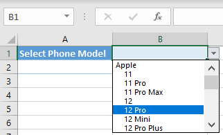
In Excel, you can create a drop-down list with items from a range of cells. Say you want to make a drop-down list of mobile phone models. If your list is long, you can add categories to make it more readable. To group a list of phone models by brand, follow these steps:
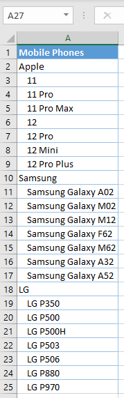
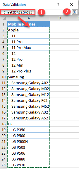
- Create a list of items grouped by category (phone models in brand groups). Insert a brand name first, then under it, each model. Add a few spaces in front of each model name. This visually indicates which models belong to which brand.
For a quick way to insert spaces, try the REPT Function or VBA.
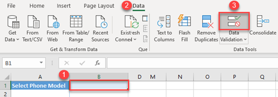
- Select the cell where you want to insert a drop-down list (B1), and in the Ribbon, go to Data > Data Validation.
- In the Data Validation window, choose List under Allow drop-down. Then click on the arrow next to the source box to select the range with list items.
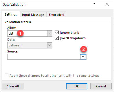
- Select the range of list items and their categories, then press Enter (or click the arrow on the right side).
- Back in the Data Validation window, click OK to confirm.
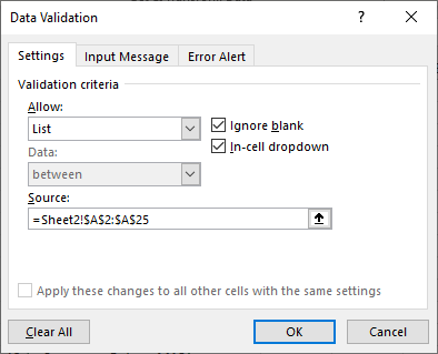
As a result, you have a drop-down list with categories in cell B2. If you click on it, you see items grouped by category.
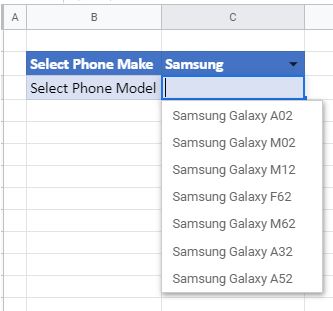
Drop Down Categories in Google Sheets
Indenting list items doesn’t work in Google Sheets. The drop-down list will display items without leading spaces. Instead, use a cascading drop-down list to create one drop down for brand and one for model.

In my previous post, I stated that one of the major problems with how most Excel users lay out their data, is using a column for each category.
In the feedback I have had from that post, it was felt that this point needed further explanation and/or an example, so I thought I would provide both here.
First of all, here is the point as it appeared in the original post (it was point number 3):
Don’t group data by putting it in different columns (THIS IS THE ONE THAT ALMOST EVERYONE GETS WRONG)
- Don’t split out financial or numerical data into separate columns to categorise the data into months, expense categories, customers, agents, etc.
- Do have one column for the financial or numerical data and create a column for month, expense category, customer or agent, to categorise each row;
- You can use data validation drop-down lists to select the appropriate category for each row;
- This one is counter-intuitive because in any report, you will almost certainly will want a column (or row) for each of these categories — but if you do this in the data you will massively restrict what you can do with it.
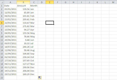
Let’s look at some sales data laid out the wrong way:

I have left out any extra data (other than the date) to keep it simple. With the data laid out like this, you could use the SUM function to calculate monthly totals, but you can’t do a lot more than that. If you were to use the data in a pivot table, you would have to add the data as 12 data fields, making it very cumbersome and inflexible.
Also, if you wanted to do any calculations on this data, such as calculating VAT, or any other Sales Tax for that matter, you would need another 12 calculated columns!
You then get into further problems if you want to analyse the data from another perspective — by salesperson for example.
A better approach
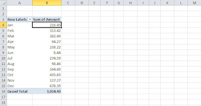
Now let’s see a better way to lay this data out:
You can also automate the month column using the following formula in cell C2:
=CHOOSE(MONTH($A2),»Jan»,»Feb»,»Mar»,»Apr»,»May»,»Jun»,»Jul»,»Aug»,»Sep»,»Oct»,»Nov»,»Dec»)
Laid out like this you can use the month as a way of analysing the amount in a pivot table for example:
Its real power however comes when you wish to add additional analysis and calculations, so for example you could add additional analysis columns for Salesperson and Country, and a VAT column (being 20% of amount):

You can then produce all manner of pivot tables, here are just a few examples:
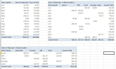
It would be just as easy to show the months as columns — the only reason I haven’t is to make best use of the space.
And remember, you can at any stage easily add further analysis or calculation columns as your reporting needs change.
I hope this has explained this point in more detail and even more importantly, highlighted the value of getting it right!
If you enjoyed this post, go to the top left corner of the blog, where you can subscribe for regular updates and your free report. If you wish to help me to provide future posts like this, please consider donating using the button in the right hand column.
Categorising string based on some words was one of my basic task in data analysis. For example, in a survey if you ask people what they like about a particular smart phone, the same answers will have a variety of words. For camera, they may use the words like photos, videos, selfies etc. They all imply camera. So it is very important to categorize sentences before, to get some meaningful information.

In this article, we will learn how to categorize in excel using keywords.
Let’s take the example of survey we talked about.
Example: Categorize Data Gathered From a Survey in Excel
So, we have done a survey about our new smartphone xyz. We have asked our customers what they like about xyz phone and captured their response in excel. Now we need to know who liked our LED screen, speaker and camera.

For this, we have prepared a list of keywords that may refer to a category, as you can see in below image. To understand, I have kept it small.
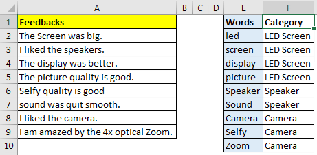
The Feedbacks is in range A2:A9, keywords are in E2:E10 and Category is in F2:F10.
The generic formula to create categories will be:
Note the curly braces, it is a array formula. Needs to be entered using CTRL+SHIFT+ENTER.
Category: It is the range that contains list of categories. Sentences or feedbacks will be categorised by these values. In our case it is F2:F10.
Words: it is the range that contains list of keywords or phrases. These will be searched in the sentences. Here it is E2:E10.
Sentence: it is the sentence that will be categorised. It is a single relative cell.
Since now we know each variable and function used for categorisation in excel, let’s implement it on our example.
In cell B2 write this formula and press CTRL+SHIFT+ENTER.
Copy down the formula to see category of each feedback.

We need to list of words and category fixed, they should not change as we copy down the formula, hence I have given absolute reference of keywords and categories. While we want sentences to change as we copy down the formula, that is why i have used relative reference of as A2. You can read understand about referencing in excel here.
Now you can prepare a report how many users liking LED screen, Speaker and Camera.
How it works?
The core of the formula is ISNUMBER(SEARCH($E$2:$E$10,A2)): I have explained it in detail here. The SEARCH function searches each value of keywords ($E$2:$E$10) in sentence of A2. It returns an array of found location of word or #VALUE (for the word not found). Finally we will have an array of 9 elements for this example. {#VALUE!;5;#VALUE!;#VALUE!;#VALUE!;#VALUE!;#VALUE!;#VALUE!;#VALUE!}. Next we use ISNUMBER Function to convert this array into useful data. It converts it into array of TRUE and FALSE. {FALSE;TRUE;FALSE;FALSE;FALSE;FALSE;FALSE;FALSE;FALSE}.
Now on, everything is simple index match. MATCH(TRUE,ISNUMBER(SEARCH($E$2:$E$10,A2)),0): the MATCH function looks for TRUE, in resulted array and returns the index of first found TRUE. which is 2 for this case.
INDEX($F$2:$F$10,MATCH(TRUE,ISNUMBER(SEARCH($E$2:$E$10,A2)),0)): Next, INDEX function looks at the 2nd position in category ($F$2:$F$10) which is LED Screen. Finally this formula categorises this text or feedback as LED screen.
Making It Case Sensitive:
To make this function case sensitive, use FIND function instead of SEARCH function. The FIND function is case sensitive by default.
The Weak Points:
1.If two of keywords are found in same sentence, sentence will be categorised according to first keyword in the list.

Capturing the text within another word. Assume we are searching for LAD in a range. Then words containing LAD will be counted. For example, Ladders will be counted for LAD since it contains LAD in it. So be careful about it. Best practice is to normalise your data as much possible.
So this was a quick tutorial about how to categorise data in excel. I tried to explain it as simple as I can. Please let me know if you have any doubt about this article or any excel related articles.
Download file:
Related Articles:
How to Check If Cell Contains Specific Text in Excel
How to Check A list of Texts In String in Excel
Get the COUNTIFS Two Criteria Match in Excel
Get the COUNTIFS With OR For Multiple Criteria in Excel
Popular Articles :
50 Excel Shortcut to Increase Your Productivity : Get faster at your task. These 50 shortcuts will make you work even faster on Excel.
How to use the VLOOKUP Function in Excel : This is one of the most used and popular functions of excel that is used to lookup value from different ranges and sheets.
How to use the COUNTIF function in Excel : Count values with conditions using this amazing function. You don’t need to filter your data to count specific values. Countif function is essential to prepare your dashboard.
How to use the SUMIF Function in Excel : This is another dashboard essential function. This helps you sum up values on specific conditions.
The multi-category chart is used when we handle data sets that have the main category followed by a subcategory. For example: “Fruits” is a main category and bananas, apples, grapes are subcategories under fruits. These charts help to infer data when we deal with dynamic categories of data sets. By using a single chart we can analyze various subcategories of data.
In this article, we will see how to create a multi-category chart in Excel using a suitable example shown below :
Example: Consider the employees from our organization working in various departments. The main categories under departments are “Marketing”, “Sales”, “IT”. Now under every department, there are multiple employees which is a subcategory.
Now, we would like to create a Multi-Category chart having the age details of employees from multiple departments. Consider the table shown below :
Table :
Employee Details Table
Implementation :
Step 1: Insert the data into the cells in Excel. Now select all the data by dragging and then go to “Insert” and select “Insert Column or Bar Chart”. A pop-down menu having 2-D and 3-D bars will occur and select “vertical bar” from it.
Select the cell -> Insert -> Chart Groups -> 2-D Column
Bar Chart Insertion
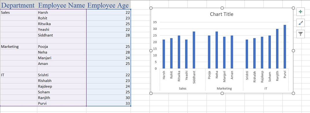
Multi-Category Chart
An important thing to note is that sometimes few subcategory data may be missing in the chart after insertion. It is not an error and just by increasing the size of the chart the data will be shown.
The Multi-category chart is ready. Now we can perform various modifications to it to make the chart more insightful by adding titles, changing the width and gap, assigning different colors to different sub-categories.
Step 2: For formatting, select the chart and use the “+” button beside it to add Title, Data labels, Axes Titles, and others or right-click and then select Format option.
- Adding Title: Check the “Chart Title” box from the Chart Elements pop down and add a suitable title.
- Adding data labels: Check the “Data Labels” from the Chart Elements pop down.
Data Labels
- Assigning a color to bars: Select the individual bar and add colors as shown below:
- Gap Width: Assign a suitable gap width as per requirements. Select all the bars, right-click on it and select “Format Data Series.”
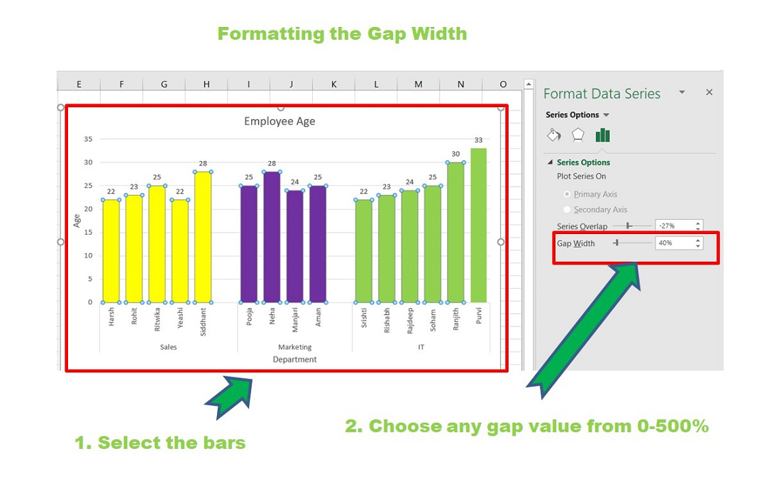
Gap width
- Formatting Axis: Select the chart and then click on the “+” button and under “Axes” select “More Options”. Another way is to select the axis in the chart and then right-click and click on “Format Axis”.
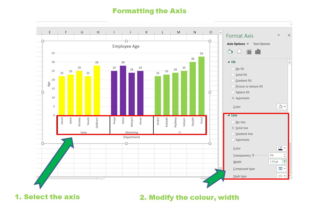
Axis Formation
- Changing the chart style: Click on the Chart Styles beside the chart and select a suitable chart style.
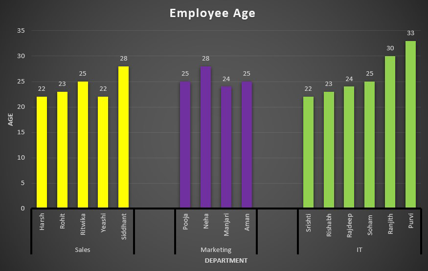
Final Multi-Category Chart
- Changing the Chart Type: Suppose now we want the above chart in the form of horizontal bars.
Select chart -> Right Click -> Change Chart Type
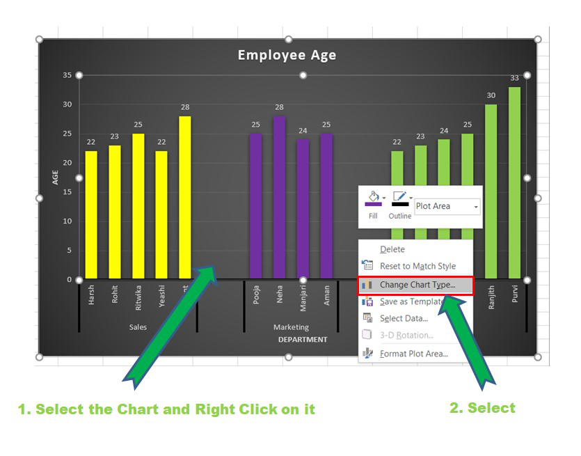
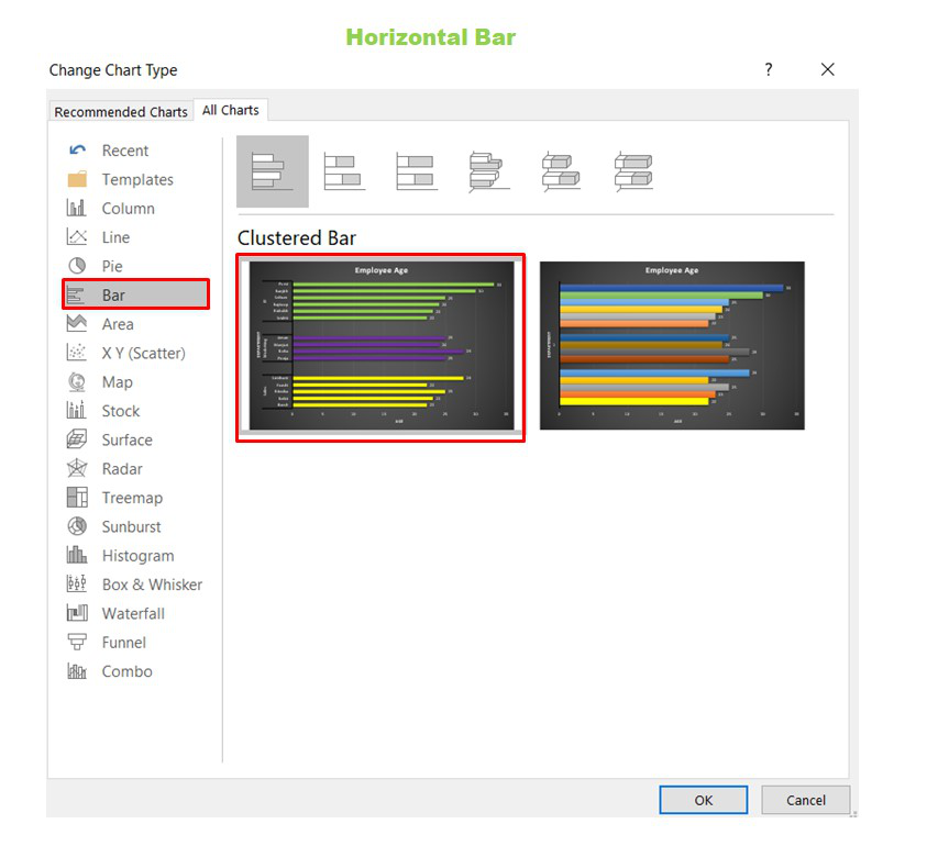
Finally, Click on OK.
Final Horizontal Multi-Category chart