How to calculate to percentage in excel

In various activities it is necessary to calculate percentages. We should understand, how do we «get» them. Trade allowances, VAT, discounts, profitability of deposits, securities and even tips — all these are calculated in the form of some part from the whole.

Let’s figure out how to work with the percentages in Excel. This program calculates automatically and admits different variants of the same formula.



Working with percentages in Excel

To count the percentage of the number, add, and take percentages on a modern calculator is not difficult. The main condition is the corresponding icon (%) on the keyboard. And only then it’s the matter of technology and mindfulness.

For example 25 + 5%. To find the value of the expression, you need to type on the calculator a given sequence of numbers and signs. The result is 26.25. With such a technique the great intellect is not needed.

To formulate formulas in Excel, let us recollect the school basics:

Percentage is one hundredth part of the whole.

To find a percentage of an integer, we should divide the required fraction by an integer and multiply by 100.

Example: 30 pieces of goods were bought. On the first day 5 units were sold. How many percentages of goods were sold?

5 is a part. 30 is an integer. We substitute data into the formula:

(5/30) * 100 = 16.7%

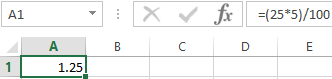
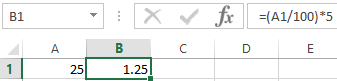
To add a percentage to a number in Excel (25 + 5%), you must first find 5% of 25. At school there was the proportion:

• 25 — 100%;
• Х — 5%.

X = (25 * 5) / 100 = 1.25

After that you can perform the addition. When the basic computing skills are restored, it is easy to understand the formulas.



How to calculate the percentage from the number in Excel

There are several ways.

Adapt the mathematical formula to the program: (Part / Whole) * 100.

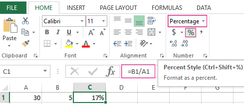
Look attentively at the formula line and the result. The result turned out to be correct. But we did not multiply by 100. Why?

In Excel the format of the cells changes. For C1, we have assigned a «Percentage» format. It means multiplying the value by 100 and putting it on the screen with the sign %. If necessary, you can set a certain number of digits after the decimal point.

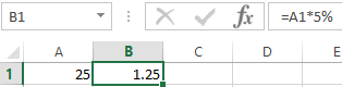
Now let’s calculate how much will be 5% of 25. To do this, enter the formula in the cell: = (25 * 5) / 100. The result is:

Another variant is = (25/100) * 5. The result will be the same.

Let’s have the example in another way by using the % sign on the keyboard:

Let us apply this knowledge to practice.

The cost of the goods and the VAT rate (18%) are known. We need to calculate the amount of VAT.

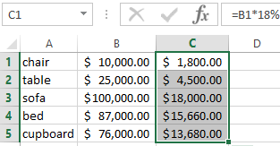
We multiply the cost of goods by 18%. Copy the formula for the whole column. To do this, we catch the mouse with the lower right corner of the cell and pull it down.

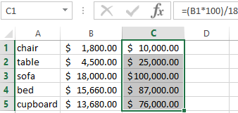
The amount of VAT, the rate is known. We should find the value of the goods. Calculation formula is: = (B1 * 100) / 18. The result is:

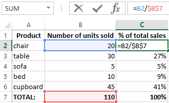
The quantity of the sold goods is known, separately and the whole. It is necessary to find the share of sales for each unit relative to the whole. The calculation formula remains the same: Part / Whole * 100. Only in this example we make the reference to the cell in the denominator of the fraction absolute. Use the $ sign in front of the line name and column name: $B$7.

How to add the percent to number

The task is solved in two actions:

1. Firstly, we find how much a percentage of the number is. Here we calculated how much will be 5% of 25.



2. Secondly, we add the result to the number. Example for review: 25 + 5%.

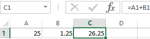
And here we performed the actual addition. Omit the intermediate effect.

The VAT rate is 18%. We need to find the amount of VAT and add it to the price of the goods. The formula is: =price + (price * 18%).

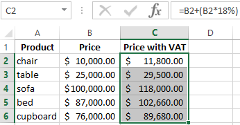
Do not forget about the brackets! With the help of it we establish the calculation procedure.

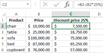
To remove the percentage from a number in Excel, you should follow the same procedure. We perform subtraction instead of addition.

How to count the odds in percentage in Excel?

What is the amount of the value changing between the two values in percentage?

First, let’s abstract from Excel. A month ago, the tables were brought to the store at a price of 100$ per unit. Today, the purchase price is 150$.

Difference in percentage is: = (New price – Old price) / Old price * 100%.

In our example, the purchase price for a unit of goods increased in 50%.

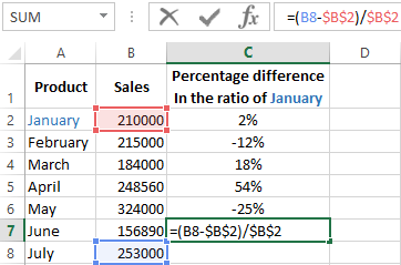
Let’s calculate the percentage difference between the data in two columns:

Do not forget to expose the «Percentage» format of the cells. Calculate the percentage difference between the lines:

The formula is as follows: =(next value – previous value) / previous value.

With such an arrangement of the data, the first line is skipped!

If you want to compare the data for all months with January, for example, use the absolute reference to the cell with the desired value ($ sign).

How to make a diagram with percentages

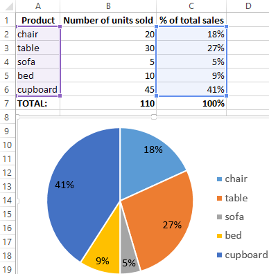
The first option is to make a column in the data table. Select 2 cell ranges A2:A6 and C2:C6 (while holding down the CTRL key). Then use this data to build a chart. Select the cells with percentages and copy — click «INSERT» — select the type of chart (for example «2D Pie») — OK.

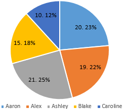
The second option: specify the format of data signatures in the form of a share. There are 22 working shifts in May. You need to calculate the percentage: the amount of work each worker did. We compose the table, where the first column is the number of working days; the second is the number of days off.

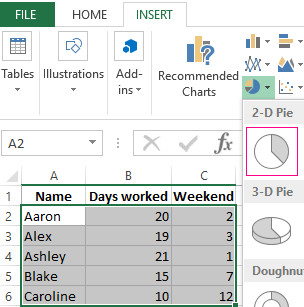
We make a pie chart. Select the data in cell ranges A2:C6. «INSERT» — «Insert Pie or Doughnut Chart» — «2D Pie».

Click on them with the right mouse button — «Add Data Labels» and «Format Data Labels»:

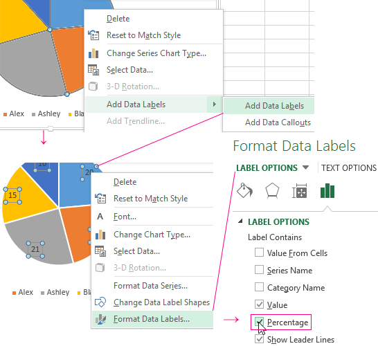
Choose «Share». On the tab «LABEL OPTIONS» we choose the percentage format. It turns out like this:

Download examples Calculate Percentages in Excel

We may stop here. And you can edit it to your taste: change the color, the appearance of the diagram, makes underscores and so on.

Anyone who constantly works with numbers probably also works with percentages. Calculating percentages apply in many areas of our day-to-day and everyday lives. Some of the areas we apply percentages include; discounts, percentage changes between different values, and percentage of correct answers in a test or survey. Lucky enough, it is easier to calculate percentages. Excel offers you different ways you can calculate percentages just as well as it does with whole numbers and decimals. The Microsoft Excel program e makes it easier by automatically applying simple, basic, or advanced formulas that allow you to add and calculate percentages in your spreadsheet.

In the article below, we will show you how to use the important formulas in excel to calculate percentage changes, discounts, and how to increase and decrease numbers by percentage.

How to calculate percentage basics

A percentage simply means out of 100, that is, a fraction of 100. You calculate it by dividing the numerator by the denominator, and the resulting figure is multiplied by 100. When you are calculating a basic percentage in excel, we use the formula:

= (part/ Total) * 100% or

= Numerator / Denominator * 100%

Remember, just like in all formulas, while calculating the percentage amount, start with an equal (=) sign.

For example, on a 15- day work leaves, Mr. S spent ten days in his hometown and five days in a vacation resort in the USA. What percentage of days did he spend on both places?

The calculations will be as follows:

Percentage formula= part days/ total days * 100%

Percentage of days spent in his hometown = 10/15* 100% = 66.66%

Percentage of days spent in the vacation resort = 5/15* 100% = 33.33%

Hence Mr. S spent 67% of his work leave in his hometown and 33% in the resort.

The example above shows how everyday percentage calculations are done. When computing these calculations using Excel, it is easier as the program performs some of the operations automatically in the background.

Let’s have a look at how percentage calculations in excel will look like;

• To calculate the percentage of the delivered items, you will enter the formula =C2/B2 manually in cell D2. Copying it down the other rows up to cell D9 will give you the decimal results.
• Click on the home tab, and look for the percentage sign in the Number group. After doing this, click on the % icon to display the decimal figures as percentages.
• In case you need to reduce or increase the number of decimal places, you can do so from the home tab in the Number group.

Note;

At times you may have a column full of percentages with many decimal places. We all know this is not standard when presenting data, for example, grades. You can easily reduce the number of decimal places by using the Format Cells feature. Here is what you will do;

• Highlight the column

• Right-click, and from the pop-up menu, select Format Cells to display a pop-up window.

• Click on the Number tab.
• Under the Category menu section, select Number, and click the down arrow that is next to Decimal Places. Click it until you get the desired number of decimal places. In the case above, we clicked up to 0.

• Click OK to display your results in the spreadsheet (the values will be rounded off to the nearest whole number).

How to calculate the percentage of a total in excel

With the above example, we have looked at the different ways you can calculate the percentages of the total. Apart from it, we have different ways one can calculate the percent of a total in excel when you are given different data sets to work with.

Example 1: calculating percentages when part of the total are in multiple rows

Let’s get to understand how this works using the example above. Suppose you have several rows of a product, and you would like to know what percentage of the total is made by orders of the particular product.

In such a scenario, the use of the SUMIF function comes in handy. The function will be used, sum up all the numbers that relate to that given product. The total of all the products will still be used as the denominator. Here is how the formula would be;

=SUMIF (range, criterion, [sum_range]) / total orders

Here is what the percentage calculation will look like in an excel spreadsheet.

In the above table, the formula is applied as follows;

Range A2:A4, the criterion is E1, sum_range B2:B4, and the total orders $B$5

The dollar signs $ creates an absolute reference to cell B10. It means that the value will not change even if the other values change according to the worksheet.

Example 2: calculating the percentage total when the totals of products ordered are provided.

At times you might come across a worksheet that has totals of your data set in a single cell at the end of a table. In such a scenario, to get the percentage of totals, you will use the given total amount as a denominator.

Let’s use the above example without including the number of items ordered.

In the table above, the denominator cell is B10. It is also referred to as the absolute reference cell. To be able to make a cell an absolute reference, you can type in the dollar sign manually or click the absolute reference cell in the formula bar and press F4. This allows you to click and drag down the other rows to get the required percentages.

How to calculate percentage change in excel rows and columns

From mathematics calculations, we all have come across percentage change calculations. When it comes to excelling, it is one of the most commonly used formulas. Percentage change works with both negative and positive values. Here we look at how to calculate percentage increase and decrease in excel.

When you are calculating the percentage change between two values, you use the formula below:

Percentage change = (New value – Old value) / Old value

It is important to take note of which values represent the new and old values when given data sets to work with.

Example 1: calculating the percentage change in an excel spreadsheet

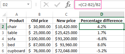
In the example below, suppose you are provided with last month’s prices (January) and this month’s (February) prices in two columns. Then to calculate the percentage change in your excel sheet, you will use the formula below:

= (Current year/week/month value – previous value) / previous value

In our case, we will use the formula = (C2 – B2) / B2

The table above applies to when you have been given values in columns and are expected to calculate the percentage change. What if you are given row data? Sometimes, you may be given data values that relate to particular days of the week, months, or even years to get the percentage change. Therefore, in situations where you have only a column of numbers in an excel sheet, this is the formula to apply:

= (first data cell – second data cell) / second data cell

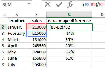
In our table below, we apply the formula = (B3 – B2) /B2 to calculate the percentage change of sales within a week in January.

Note:

When calculating the percentage growth, we skip the first-row cell of the percentage changes. We do leave it blank because it is not being used in the comparison of the given values.

How to create a custom number format

At times you may want to customize the appearance of numbers. You may decide to make the percentage decrease, which are the negative values to stand out in red. You may also decide to customize your positive values to be green. Here are the steps to follow;

1. Highlight the percentage change column in which you want to apply the customized format.

2. Go to the Home tab, click on the drop-down arrow in the Numbers command group.

3. on the drop-down box, click on the More Number Formats option arrow.

4. In the Format Cells pop-up window, click on the Number tab.

5. Select Custom under the category section. Use one of the existing codes as a starting point to create and save your customized format.

6.
Click OK, and the new format will be applied to the highlighted column.

How to calculate and apply a percentage increase or decrease to values in Excel

At times you may have a budget set aside for certain expenses. Due to unavoidable circumstances, the funds allocated towards the different activities may either increase or reduce. For accountability purposes, you will need to calculate the increase or decrease amounts.

To increase an amount by a percentage, apply the formula below:

= Amount * (1 + % increase)

To decrease a current amount by percentage, use the formula

= Amount * (1 – % decrease)

Let’s have a look at how you can increase or decrease given values by a percentage.

Example:

Suppose you have been given a column of sales value you are supposed to increase or reduce by a certain percentage. It is good to have the updated values in one column rather than have a different column where the formula appears.

Let’s look at the steps to be followed to arrive at the expected results.

1. In one column, enter all the sales amount values you want to increase or decrease.

2. enter the formula that applies in an empty cell. That is, enter either the increase or decrease formula.

3. Select the cell with the formula and copy it. You can use the shortcut Ctrl + C or by right-clicking and selecting Copy.

4. Select the range of cells you want the increase or decrease applied to.

5. Right-click the selected cells and then click on the Paste Special feature to display a dialog window.

6. In the Window, under the paste category, select Values. In the Operation category, select multiply.

7. Click OK to display your results.

Note;

We use parentheses in the formula when calculating any percentage changes due to an increase or decrease in a given amount. By default, Excel operations state that multiplication must be done before addition or subtraction. Letting this happen in the above formula may lead to you getting the wrong results. Therefore, as in the formula, the second part is wrapped in parentheses to ensure that the multiplication part is calculated last.

Calculating and finding percentiles in excel

When working with percentages, you may have to calculate the percentile rank of a given data set. The percentile rank of a given number is where it falls in a range of different numbers. In excel, it is easier to calculate percentile rank as there are functions available to make your work easier. The two functions in excel are:

=PERCENTILE. EXC (array, value)

=PERCENTILE. INC (array value)

The functions above include the same arguments. These are:

• Array- this argument is the range of numbers that you are looking for in a percentile.
• Value-this argument represents the percentile rank you are looking for.

Example

Suppose you are given percentage scores of a class. Find the 60th percentile.

To get the solution below, we use the formula =PERCENTILE.INC (B2:B5, .6)

How to calculate the Discount Rate or Price in Excel spreadsheets

During special occasions globally, most sellers and supermarkets always offer their products at discounts. It may be Christmas, Easter, or Thanksgiving holiday, or it may be an anniversary for the shop. So you may get as high as a 70% discount to as low as a 100% discount. But what if you plan on purchasing a lot of products offered at a discount and you need to know the different discount rates and prices you will pay? There is no reason to be frustrated as with excel, and you can easily calculate the discount rates and prices.

Here is a step-by-step guide on how to calculate discount rates in excel when given the initial price and the current selling price.

1. In an excel worksheet, in one column, type in the initial price values of the product. In the second column, you will type in the current sales price, while the third column will be discount rates.

2. To get the discount rate of the first product, type in the empty cell the formula = (C2-B2)/B2. Where B2 indicates the original price, C2 represents the current sales price.

3. Press the Enter button to get the resulting discount rate of that product. To fill in the other blanks, drag the fill handle to fill the above formula to the other empty cells.

4. Remember, your values will be in decimal places, and therefore, you will need to convert them into percentages and adjust the number of decimals.

What if you have been given the discount rate as it is on many occasions and told to calculate the current selling price of an item?

Follow these steps

1. Select the first blank cell on the selling price column.

2. Type in the formula =B2- (B2*C2) where B2 represents the original price, and C2 is the discount rate of each item.

3. Press the Enter button and drag the fill handle to fill in the other empty cells. The selling price figures will be shown in the empty cells as shown below.

How to calculate percentage profit in Excel

When we talk about profits, we refer to the financial benefits that a business or company remains with after paying all its expenses. Profit percentage calculation is an important tool in any business setting. It is a common tool as it helps measure the profitability of a business. A business uses the percentage to measure its ability to convert its sales into profits. A company also uses profits to gauge the capacity of a business to continue its operations in the foreseeable future. Therefore, it is a vital computation in any business. Profit is calculated and expressed as a percentage of the selling price. In Excel, there are two types of profit percentages;

• Profit margin-it is the percentage you get on the selling price. The formula is;

Profit Margin = (Profit/ Cost Price) * 100

• Markup- it is calculated as the percentage of the cost price. The formula is;

% Markup = (Profit/ Cost Price) * 100

Example: Excel profit percentage calculation

Suppose you are the owner of a retail shop, and due to the heavy demand during the Christmas season, you purchase 150 pieces of refrigerated turkey at the rate of 35 per bird. You also purchase 80 bottles of wine at the rate of 115 per bottle. Due to the high costs of transportation expenses incurred, $2500, you decide to sell the turkey at $50 per bird and a wine bottle at $150. Apart from this, you offer your customers a discount of 5% on any product purchased from your retail shop. What will be your total profit on the two products?

Here are the steps to be followed to get the profit amount;

• To get the profit, you first have to calculate the total sales and cost. We use the formula ;

Profit = Total Sales- Total Cost

In our excel spreadsheet, the total cost will be the sum of the transportation costs, the turkey’s total cost, and the wine’s total cost. The total sales will be the sum of the net sales of the turkey and the net sales of the wine. When you want to get the net sales, we will minus the discount rate amount from the selling price. To get the profit as in our figure below, we use the formula = B10-B5.

• To get the percentage profit, we use the formula = (Profit/ Total cost) * 100. From the example above, our formula will be

Profit % = (B12/B5) *100

Conclusion

As seen above, Microsoft Excel formulas for percentages are crucial in our everyday life. Even if percentages have never been your favorite calculations to perform, with the above basic excel formulas, you can hack them and get excel to do your computations. Take note that these are just some of the basic excel percent formulas. You can also decide to dive into the advanced percentages like variance, interest rates percentage, etc.

These are some of the most common questions and challenges that people have. I get asked so today I have simplified it and laid it all out in a post for you. You’re welcome!

1.  Percentages vs Numbers

The first thing to understand is the correlation between percentages and numbers. Think of it like this:

2. Common mistake: Formatting percentages rather than calculating percentages

Consider the following range of numbers:

3. How to calculate percentages the proper way

a) Example #1: How to add 20% Sales Tax

=SUM(A1,A1*B1)

b) Example #2:Using percentages to remove sales tax from a total

=E1/(100%+B1)

This equates to 

=E1/120%

c) Example #3: Using percentages to calculate interest on a loan

=A1*A2

5. What next?