How to calculate irr in excel

IRR (Internal Rate of Return) is an indicator of the internal rate of return of an investment project. It is often used to compare different proposals for the growth and profitability perspective. The higher the IRR, the greater is the growth prospects for this project. Let’s calculate the interest rate of IRR in Excel.



The economic meaning of the indicator

Other names: the internal rate of profitability (profit, discount), the internal factor of recoupment (efficiency), an internal norm.

The IRR coefficient shows the minimum level of profitability of the investment project. In another way: it is the interest rate at which the net present value is zero.

The formula for calculating the indicator manually:

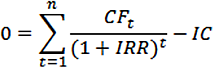
• CFt – is cash flow for a certain period of time t;
• IC – is investments in the project at the stage of entry (launch);
• t – is the time period.

In practice, the IRR ratio is often compared with the weighted average capital cost (WACC):

1. IRR above WACC: this project should be carefully considered.
2. IRR below WACC: it is inappropriate to invest in the development of the project.
3. Indicators are equal: the minimum permissible level (the enterprise needs to adjust the cash flow).

Often the IRR is compared in percentages on a bank deposit. If the interest on the deposit is higher, then it is better to look for another investment project.



Example of calculating IRR in Excel

You can quickly calculate the IRR using the built-in Excel IRR function. Syntax:

1. Range of values — reference to cells with numerical arguments for which you want to calculate the internal rate of return (at least one cash flow must have a negative value).
2. Assumption — a value that is supposedly close to the value of the IRR (the argument is optional; but if the function produces an error, the argument must be specified).

Take the conventional figures:

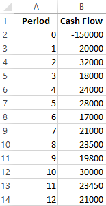
The initial costs were 150,000, so this numerical value entered the table with a minus sign. Now we’ll find the IRR. The formula for calculation in Excel:

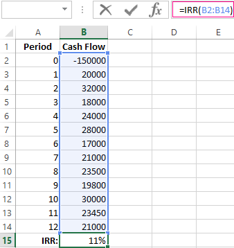
Calculations showed that the internal rate of return on the investment project is 11%. For further analysis, the value is compared with the interest rate of the bank deposit, or the cost of the capital of the project, or IRR of another investment project.

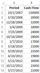
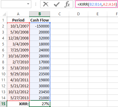
We calculated the IRR for regular cash income. The IRR function cannot be used with non-systematic income because the discount rate for each cash flow will vary. We solve the problem with the help of the function XIRR.

We modify the table with the initial data for the example:

The mandatory arguments of the XIRR function are next:

• Values are cash flows;
• Dates are an array of dates in the appropriate format.

The formula for calculating IRR for non-systematic payments:

A significant drawback of the two previous functions is the unrealistic assumption about the rate of reinvestment. It is recommended to use the MIRR function to correctly consider the assumption of reinvestment.

Arguments:

• Values are payments;
• Financing rate is interest paid for funds in circulation;
• The rate of reinvestment.

Suppose that the discount is 10%. There is a possibility of reinvesting the revenues at a rate of 7% per annum. We calculate the modified internal rate of return:

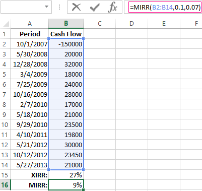
The resulting rate of return is three times less than the previous result. And it’s below the financing. Therefore, the profitability of this project is doubtful.

Graphical method for calculating IRR in Excel

The IRR value can be found graphically by plotting the net present value (NPV) versus the discount rate. NPV is one of the methods for evaluating an investment project which is based on the methodology of discounting cash flows.

For example, take a project with the following structure of cash flows:

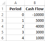
You can use the NPV function to calculate NPV in Excel:

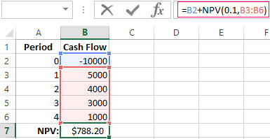
Since the first cash flow occurred in the zero periods, it does not have to enter the value array. The initial investment should be added to the value calculated by the NPV function.

The function discounted cash flows for periods from 1 to 4 at a rate of 10% (0.10). It is impossible to accurately determine the discount rate and all cash flows when analyzing a new investment project. It makes sense to look at the dependence of NPV on these indicators. In particular, look how it depends on the cost of capital (discount rates).

We calculate NPV for different discount rates:

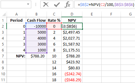
Let’s see the results on the chart:

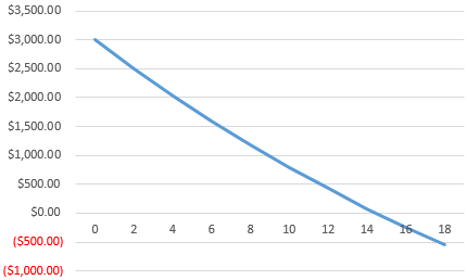
Remember that the IRR is the discount rate at which the NPV of the analyzed project is zero. Therefore, the intersection point of the NPV graph with the abscissa axis is the internal profitability of the enterprise.

This article describes the formula syntax and usage of the IRR function in Microsoft Excel.

Description

Returns the internal rate of return for a series of cash flows represented by the numbers in values. These cash flows do not have to be even, as they would be for an annuity. However, the cash flows must occur at regular intervals, such as monthly or annually. The internal rate of return is the interest rate received for an investment consisting of payments (negative values) and income (positive values) that occur at regular periods.

Syntax

IRR(values, [guess])

The IRR function syntax has the following arguments:

• Values    Required. An array or a reference to cells that contain numbers for which you want to calculate the internal rate of return.

  • Values must contain at least one positive value and one negative value to calculate the internal rate of return.

  • IRR uses the order of values to interpret the order of cash flows. Be sure to enter your payment and income values in the sequence you want.

  • If an array or reference argument contains text, logical values, or empty cells, those values are ignored.

• Guess    Optional. A number that you guess is close to the result of IRR.

  • Microsoft Excel uses an iterative technique for calculating IRR. Starting with guess, IRR cycles through the calculation until the result is accurate within 0.00001 percent. If IRR can’t find a result that works after 20 tries, the #NUM! error value is returned.

  • In most cases you do not need to provide guess for the IRR calculation. If guess is omitted, it is assumed to be 0.1 (10 percent).

  • If IRR gives the #NUM! error value, or if the result is not close to what you expected, try again with a different value for guess.

Remarks

IRR is closely related to NPV, the net present value function. The rate of return calculated by IRR is the interest rate corresponding to a 0 (zero) net present value. The following formula demonstrates how NPV and IRR are related:

NPV(IRR(A2:A7),A2:A7) equals 1.79E-09 [Within the accuracy of the IRR calculation, the value is effectively 0 (zero).]

Example

Copy the example data in the following table, and paste it in cell A1 of a new Excel worksheet. For formulas to show results, select them, press F2, and then press Enter. If you need to, you can adjust the column widths to see all the data.

Data	Description
-$70,000	Initial cost of a business
$12,000	Net income for the first year
$15,000	Net income for the second year
$18,000	Net income for the third year
$21,000	Net income for the fourth year
$26,000	Net income for the fifth year
Formula	Description	Result
=IRR(A2:A6)	Investment’s internal rate of return after four years	-2.1%
=IRR(A2:A7)	Internal rate of return after five years	8.7%
=IRR(A2:A4,-10%)	To calculate the internal rate of return after two years, you need to include a guess (in this example, -10%).	-44.4%

What Is the Internal Rate of Return (IRR)?

The internal rate of return (IRR) is the discount rate providing a net value of zero for a future series of cash flows. Both the IRR and net present value (NPV) are used when selecting investments based on their returns.

Excel has three functions for calculating the internal rate of return that include Internal Rate of Return (IRR), Modified Internal Rate of Return (MIRR), and Internal Rate of Return with time periods (XIRR).

The IRR function calculates the internal rate of return for a series of cash flows, the MIRR function works with interest rates for borrowing and investing, and the XIRR function calculates a more accurate internal rate of return as it considers time periods.

What Is Net Present Value?

NPV is the difference between the present value of cash inflows and the present value of cash outflows over time.

The net present value of a project depends on the discount rate used. So when comparing two investment opportunities, the choice of the discount rate, which is often based on a degree of uncertainty, will have a considerable impact.

In the example below, using a 20% discount rate, investment #2 shows higher profitability than investment #1. When opting instead for a discount rate of 1%, investment #1 shows a return bigger than investment #2. Profitability often depends on the sequence and importance of the project’s cash flow and the discount rate applied to those cash flows.

How IRR and NPV Differ

The main difference between the IRR and NPV is that NPV is an actual amount while the IRR is the interest yield as a percentage expected from an investment.

Investors typically select projects with an IRR that is greater than the cost of capital. However, selecting projects based on maximizing the IRR as opposed to the NPV could result in suboptimal economic outcomes.

IRR represents the actual annual return on investment only when the project generates zero interim cash flows, or if those investments can be invested at the current IRR.

Calculating IRR in Excel

The IRR is the discount rate that can bring an investment’s NPV to zero. When the IRR has only one value, this criterion becomes more interesting when comparing the profitability of different investments.

In our example, the IRR of investment #1 is 48% and, for investment #2, the IRR is 80%. This means that in the case of investment #1, with an investment of $2,000 in 2013, the investment will yield an annual return of 48%. In the case of investment #2, with an investment of $1,000 in 2013, the yield will bring an annual return of 80%.

If no parameters are entered, Excel starts testing IRR values differently for the entered series of cash flows and stops as soon as a rate is selected that brings the NPV to zero. If Excel does not find any rate reducing the NPV to zero, it shows the error «#NUM.»

If the second parameter is not used and the investment has multiple IRR values, we will not notice because Excel will only display the first rate it finds that brings the NPV to zero.

In the image below, for investment #1, Excel does not find the NPV rate reduced to zero, so we have no IRR. 

The image below also shows investment #2. If the second parameter is not used in the function, Excel will find an IRR of -10%. On the other hand, if the second parameter is used (i.e., = IRR ($ C $ 6: $ F $ 6, C12)), there are two IRRs rendered for this investment, which are -10% and 216%.

If the cash flow sequence has only a single cash component with one sign change (from + to — or — to +), the investment will have a unique IRR. However, most investments begin with a negative flow and a series of positive flows as the first investments come in. Profits then, hopefully, subside, as was the case in our first example.

In the image below, we calculate the IRR. To do this, we simply use the Excel IRR function:

Calculating MIRR in Excel

When a company uses different borrowing rates of reinvestment, the modified internal rate of return (MIRR) applies.

In the image below, we calculate the IRR of the investment as in the previous example but taking into account that the company will borrow money to plow back into the investment (negative cash flows) at a rate different from the rate at which it will reinvest the money earned (positive cash flow). The range C5 to E5 represents the investment’s cash flow range, and cells D10 and D11 represent the rate on corporate bonds and the rate on investments.

The image below shows the formula behind the Excel MIRR. We calculate the MIRR found in the previous example with the MIRR as its actual definition. This yields the same result: 56.98%. 



(

−

NPV

(

rrate, values

[

positive

]

)

×

(

1

+

rrate

)

n

NPV

(

frate, values

[

negative

]

)

×

(

1

+

frate

)

)

1

n

−

1

−

1

begin{aligned}left(frac{-text{NPV}(textit{rrate, values}[textit{positive}])times(1+textit{rrate})^n}{text{NPV}(textit{frate, values}[textit{negative}])times(1+textit{frate})}right)^{frac{1}{n-1}}-1end{aligned}

(NPV(frate, values[negative])×(1+frate)−NPV(rrate, values[positive])×(1+rrate)n​)n−11​−1​        

Calculating XIRR in Excel

The XIRR function takes into consideration different periods. To use this function, Excel requires both the cash flow amounts as well as the dates on which those cash flows are paid.

In the example below, the cash flows are not disbursed at the same time each year – as is the case in the above examples. Rather, they are happening at different periods. We use the XIRR function below to solve this calculation. We first select the cash flow range (C5 to E5) and then select the range of dates on which the cash flows are realized (C32 to E32).

For investments with cash flows received or cashed at different moments in time for a firm that has different borrowing rates and reinvestments, Excel does not provide functions that can be applied to these situations although they are probably more likely to occur.

Is this article up to date?