How to calculate in excel hours

Add time

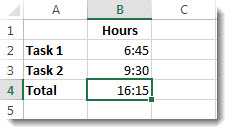
Suppose that you want to know how many hours and minutes it will take to complete two tasks. You estimate that the first task will take 6 hours and 45 minutes and the second task will take 9 hours and 30 minutes.

Here is one way to set this up in the a worksheet.

1. Enter 6:45 in cell B2, and enter 9:30 in cell B3.

2. In cell B4, enter =B2+B3 and then press Enter.

   

   The result is 16:15—16 hours and 15 minutes—for the completion the two tasks.

   Tip: You can also add up times by using the AutoSum function to sum numbers. Select cell B4, and then on the Home tab, choose AutoSum. The formula will look like this: =SUM(B2:B3). Press Enter to get the same result, 16 hours and 15 minutes.

Well, that was easy enough, but there’s an extra step if your hours add up to more than 24. You need to apply a special format to the formula result.

To add up more than 24 hours:

1. In cell B2 type 12:45, and in cell B3 type 15:30.

2. Type =B2+B3 in cell B4, and then press Enter.

   

   The result is 4:15, which is not what you might expect. This is because the time for Task 2 is in 24-hour time. 15:30 is the same as 3:30.

3. To display the time as more than 24 hours, select cell B4.

4. On the Home tab, in the Cells group, choose Format, and then choose Format Cells.

   

5. In the Format Cells box, choose Custom in the Category list.

6. In the Type box, at the top of the list of formats, type [h]:mm;@ and then choose OK.

   Take note of the colon after [h] and a semicolon after mm.

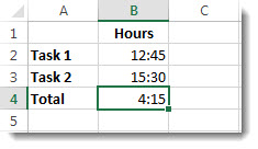
The result is 28 hours and 15 minutes. The format will be in the Type list the next time you need it.

Subtract time

Here’s another example: Let’s say that you and your friends know both your start and end times at a volunteer project, and want to know how much time you spent in total.

Follow these steps to get the elapsed time—which is the difference between two times.

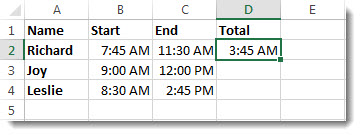
1. In cell B2, enter the start time and include “a” for AM or “p” for PM. Then press Enter.

2. In cell C2, enter the end time, including “a” or “p” as appropriate, and then press Enter.

3. Type the other start and end times for your friends, Joy and Leslie.

4. In cell D2, subtract the end time from the start time by entering the formula =C2-B2, and then press Enter.

   

5. In the Format Cells box, click Custom in the Category list.

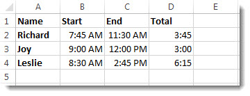
6. In the Type list, click h:mm (for hours and minutes), and then click OK.

   Now we see that Richard worked 3 hours and 45 minutes.

   

7. To get the results for Joy and Leslie, copy the formula by selecting cell D2 and dragging to cell D4.

   The formatting in cell D2 is copied along with the formula.

To subtract time that’s more than 24 hours:

It is necessary to create a formula to subtract the difference between two times that total more than 24 hours.

Follow the steps below:

1. Referring to the above example, select cell B1 and drag to cell B2 so that you can apply the format to both cells at the same time.

2. In the Format Cells box, click Custom in the Category list.

3. In the Type box, at the top of the list of formats, type m/d/yyyy h:mm AM/PM.

   Notice the empty space at the end of yyyy and at the end of mm.

   The new format will be available when you need it in the Type list.

4. In cell B1, type the start date, including month/day/year and time using either “a” or “p” for AM and PM.

   

5. In cell B2, do the same for the end date.

6. In cell B3, type the formula =(B2-B1)*24.

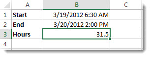
The result is 31.5 hours.

Note: You can add and subtract more than 24 hours in Excel for the web but you cannot apply a custom number format.

Add time

Suppose you want to know how many hours and minutes it will take to complete two tasks. You estimate that the first task will take 6 hours and 45 minutes and the second task will take 9 hours and 30 minutes.

1. In cell B2 type 6:45, and in cell B3 type 9:30.

2. Type =B2+B3 in cell B4, and then press Enter.

It will take 16 hours and 15 minutes to complete the two tasks.

Tip: You can also add up times using AutoSum. Click in cell B4. Then click Home > AutoSum. The formula will look like this: =SUM(B2:B3). Press Enter to get the result, 16 hours and 15 minutes.

Subtract time

Say you and your friends know your start and end times at a volunteer project, and want to know how much time you spent. In other words, you want the elapsed time or the difference between two times.

1. In cell B2 type the start time, enter a space, and then type “a” for AM or “p” for PM, and press Enter. In cell C2, type the end time, including “a” or “p” as appropriate, and press Enter. Type the other start and end times for your friends Joy and Leslie.

2. In cell D2, subtract the end time from the start time by typing the formula: =C2-B2, and then pressing Enter. Now we see that Richard worked 3 hours and 45 minutes.

   

3. To get the results for Joy and Leslie, copy the formula by clicking in cell D2 and dragging to cell D4. The formatting in cell D2 is copied along with the formula.

   

If you’ve been relying on Excel to manage your projects and need help with time calculations, you’re not alone. Figuring out the elapsed time of a project or task is crucial for team leads that need to know what work should be prioritized and how to properly allocate resources.

Simply put, time values are tricky in Excel—especially when calculating time difference, hours worked, or the difference between two employees.

Luckily for you, we’ve done all the hard work to help format cells and calculate elapsed time in Excel faster. Let’s get confident about using Excel for project time tracking and discover the various ways of figuring time.

Types of Time Calculations in Excel

There isn’t a single formula or format for calculating time in Excel. It depends on your dataset and the goal you want to achieve. Most use a custom format (number over text function) to understand time and date values, or the time difference value.

But there are two types of calculations to get you started, which include:

• Add time: If you need to obtain the sum of two time values to get a total
  • Add up to less than 24 hours: When you need to know how many hours and minutes it’ll take to complete two simple tasks
  • Add up to more than 24 hours: When you need to add the estimated or actual elapsed time of multiple slow, complex tasks
• Subtract time: If you need to get the total time between a start and end times
  • Subtract times whose difference is less than 24 hours: When you need to figure out the hours elapsed since a team member started to execute a simple task
  • Subtract times whose difference is more than 24 hours: When you need to know the hours that have gone by since your project started

Let’s go through a few formulas for time calculations in Excel so you get down to the exact hours, minutes, and seconds in your custom time format.

Time Difference in Excel

Before we teach you how to calculate time in Excel, you must understand what time values are in the first place. Time values are the decimal number to which Excel applied a time format to make them look like times (i.e., the hours, minutes, and seconds).

Because Excel times are numbers, you can add and subtract them. And the difference between a start time and an end time is called “time difference” or “elapsed time.”

These are the steps to subtract times whose difference is less than 24 hours:

1. Enter the start date and time in cell A2 and hit Enter. Don’t forget to write “AM” or “PM”
2. Enter the end time in cell B2 and hit Enter
3. Enter the formula =B2-A2 in cell C2 and hit Enter.

^WARNING
As you can tell from the figure, this formula doesn’t work for times that belong to different days. This example shows the time difference between two time values within a 24-hour time period.

4. Right-click on C2 and select Format Cells.

5. Choose the Custom category and type “h:mm”

^{SIDE NOTE}
You might wish to obtain the time difference expressed in hours or hours, minutes, and seconds. If so, type “h” or “h:mm:ss,” respectively. This will help you avoid negative time values.

6. Click OK to see the total change to a format describing only the number of hours and minutes in the elapsed time between A2 and B2.

Check out our detailed blog to find a list of time management strategies you can use right away!

Date and time in Excel

In the previous section, you learned how to calculate hours in Excel. But the formula you learned only applied to time differences of less than 24 hours.

If you need to subtract times whose difference is more than 24 hours, you need to work with dates besides times. Do it like this (format cells dialog box):

1. Enter the start time in cell A2 and hit Enter.
2. Enter the end time in cell B2 and hit Enter.
3. Right-click on A2 and select Format Cells.
4. Choose the Custom category and type “m/d/yyyy h:mm AM/PM.”
5. Click OK to see A2 change to a format starting with “1/0/1900” and adjust the date.
6. Use the Format Painter to copy the formatting of A2 to B2 and adjust the date.
7. Enter the formula =(B2-A2)*24 in cell C2 and hit Enter to see the total change to a format describing the number of hours in the time elapsed between A2 and B2.

^WARNING
You must apply the “Number” format to C2 to get the correct value in the above formula.

Sum time in Excel

Suppose you want to sum up the time difference between your team members working on multiple project tasks. If those durations add up to less than 24 hours, follow these steps:

1. Enter one duration in cell B2 (with the format h:mm) and hit Enter.
2. Enter the other duration in cell B3 and hit Enter.
3. Enter the formula =B2+B3 in cell B4 and hit Enter.

^{PRO TIP}
If you prefer clicking a single button instead of entering a formula, you may position the cursor in B4 and hit the Σ (or AutoSum) button in the Home tab. The button will apply the formula =SUM(B2:B3) to the cell in the above example.

If the total duration of your project tasks adds up to more than 24 hours, follow these steps instead:

1. Enter one duration in cell B2 (with the format h:mm) and hit Enter. (Warning: Beware that the maximum duration is 23 hours and 59 minutes)
2. Enter the other duration in cell B3 and hit Enter.
3. Enter the formula =B2+B3 in cell B4 and hit Enter.
4. Right-click on B4 and select Format Cells.
5. Choose the Custom category and type “[h]:mm;@.”
6. Click OK to see B4 correctly displaying the sum of the times in B2 and B3.

If you’d like to know more about Excel project management, our blog is the perfect place to start!

The Complete List of Formulas for Calculating Time in Excel

It pays to know the formulas when you’re calculating time difference in Excel. To get your time difference and value set up correctly, we’ve provided a list of formulas to make your calculations easier.

Formula	Description
=B2-A2	Difference between the two time values in cells A2 and B2
=(B2-A2)*24	Hours between the value in cells A2 and B2 (24 being the number of hours in a day)  Warning: If the difference is 24+ hours, you must apply the “Custom” format with the type “m/d/yyyy h:mm AM/PM” to A2 and B2. You also must apply the “Number” format to the cell containing the time difference formula.
=TIMEVALUE(“8:02 PM”)-TIMEVALUE(“9:15 AM”)	Warning: The difference must be less than 24 hours.
=TEXT(B2-A2,”h”)	Hours between the values in cells A2 and B2  Warning: You must apply the “Custom” format with the type “h” to A2 and B2. Also, the value in B2 cannot be less than A2 and the difference must be less than 24 hours to avoid a negative value. And the TEXT function returns a textual value.
=TEXT(B2-A2,”h:mm”)	Minutes and hours between the time values in cells A2 and B2.  Warning: You must apply the “Custom” format with the type “h:mm” to A2 and B2. Also, the value in B2 cannot be less than A2 and the difference must be less than 24 hours.
=TEXT(B2-A2,”h:mm:ss”)	Hours, minutes, and seconds between the time values in cells A2 and B2.  Warning: You must apply the “Custom” format with the type “h:mm:ss” to A2 and B2. And the value in B2 cannot be less than A2 and the difference must be less than 24 hours.
=INT((B2-A2)*24)	Number of complete hours between the time values in cells A2 and B2 (24 being hours in a day).  Warning: If the difference is 24+ hours, you must apply the “Custom” format with the type “m/d/yyyy h:mm AM/PM” to A2 and B2. And you must apply the “Number” format to the cell containing the time difference formula.
=(B2-A2)*1440	Minutes between the time values in cells A2 and B2 (1440 being minutes in a day). Warning: If the difference is 24+ hours, you must apply the “Custom” format with the type “m/d/yyyy h:mm AM/PM” to A2 and B2. And you must apply the “Number” format to the cell containing the time difference formula.
=(B2-A2)*86400	Seconds between the time values in cells A2 and B2 (86400 being the seconds in a day).   Warning: If the difference is 24+ hours, you must apply the “Custom” format with the type “m/d/yyyy h:mm AM/PM” to A2 and B2. And you must apply the “Number” format to the cell containing the time difference formula.
=HOUR(B2-A2)	Hours between the time values in cells A2 and B2. Warning: The value in B2 cannot be less than the value in A2 and the difference must be less than 24 hours. Also, the HOUR function returns a numeric value.
=MINUTE(B2-A2)	Minutes between the time values in cells A2 and B2.  Warning: The value in B2 cannot be less than the value in A2 and the difference must be less than 60 minutes. Also, the MINUTE function returns a numeric value.
=SECOND(B2-A2)	Seconds between the time values in cells A2 and B2.  Warning: The value in B2 cannot be less than the value in A2 and the difference must be less than 60 seconds. Also, the SECOND function returns a numeric value.
=NOW()-A2	Time elapsed between the date and time in cell A2 and the current date and time.  Warning: If the elapsed time is 24+ hours, you must apply the “Custom” format with the type “d “days” h:mm:ss” to the cell containing the time difference formula. Also, Excel doesn’t update the elapsed time in real-time. To do that, you must hit Shift+F9.
=TIME(HOUR(NOW()),MINUTE(NOW()),SECOND(NOW()))-A2	Time elapsed between the value in cell A2 and the current date and time.  Warning: Excel doesn’t update the elapsed time in real-time. To do that, you must hit Shift+F9.
=INT(B2-A2)&” days, “&HOUR(B2-A2)&” hours, “&MINUTE(B2-A2)&” minutes, and “&SECOND(B2-A2)&” seconds”	Time elapsed between the date and time or time values in cells A2 and B2, expressed in the format “dd days, hh hours, mm minutes, and ss seconds.”  Warning: This formula returns a textual value. If you need the result to be a value, use the formula =B2-A2 and apply the “Custom” format with the type “d “days,” h “hours,” m “minutes, and” s “seconds”” to the cell containing the time difference formula.
=IF(INT(B2-A2)>0,INT(B2-A2)&” days,”,””)&IF(HOUR(B2-A2)>0,HOUR(B2-A2)&” hours,”,””)&IF(MINUTE(B2-A2)>0,MINUTE(B2-A2)&” minutes, and “,””)&IF(SECOND(B2-A2)>0,SECOND(B2-A2)&” seconds”,””)	Time elapsed between the date and time or values in cells A2 and B2, expressed in the format “dd days, hh hours, mm minutes, and ss seconds” with zero values hidden.  Warning: This formula returns a textual value. If you need the result to be a value, use the formula =B2-A2 and apply the “Custom” format with the type “d “days,” h “hours,” m “minutes, and” s “seconds”” to the cell containing the time difference formula.
=A2+TIME(1,0,0)	Value in cell A2 plus one hour.  Warning: This formula only allows adding less than 24 hours to a value.
=A2+(30/24)	Value in cell A2 plus 30 hours (24 being hours in a day).  Warning: This formula allows adding any number of hours to a value.
=A2-TIME(1,0,0)	Time value in cell A2 minus one hour.  Warning: This formula only allows subtracting less than 24 hours from a value.
=A2-(30/24)	Time value in cell A2 minus 30 hours.  Warning: This formula allows subtracting any number of hours from a value.
=A2+TIME(0,1,0)	Time value in cell A2 plus one minute.  Warning: This formula only allows adding less than 60 minutes to a value.
=A2+(100/1440)	Time value in cell A2 plus 100 minutes (1440 being minutes in a day).  Warning: This formula allows adding any number of minutes to a value.
=A2-TIME(0,1,0)	Time value in cell A2 minus one minute.  Warning: This formula only allows subtracting less than 60 minutes from a value.
=A2-(100/1440)	Time value in cell A2 minus 100 minutes.  Warning: This formula allows subtracting any number of minutes from a value.
=A2+TIME(0,0,1)	Time value in cell A2 plus one second.  Warning: This formula only allows adding less than 60 seconds to a value.
=A2+(100/86400)	Time value in cell A2 plus 100 seconds (86400 being seconds in a day). Warning: This formula allows adding any number of seconds to a value.
=A2-TIME(0,0,1)	Time value in cell A2 minus one second.  Warning: This formula only allows subtracting less than 60 seconds from a value.
=A2-(100/86400)	Time value in cell A2 minus 100 seconds.  Warning: This formula allows subtracting any number of seconds from a value.
=A2+B2 =SUM(A2:B2)	Total hours, hours and minutes, or hours, minutes, and seconds in the values from cells A2 and B2, depending on the format you applied to those cells.  Warning: If the total adds up to more than 24 hours, you must apply the “Custom” format with the type “[h]:mm;@” to the cell containing the SUM formula.

An Easier Alternative to Calculating Time in Excel

Although the formulas in this article work, there’s a better way to calculate time—ClickUp!

Sure, spreadsheets are great for managing data, but what about your day-to-day tasks? And how do you communicate with your team to show these times in a simple and clear way?

ClickUp’s Table view keeps track of all your tasks, including assignees, status, and due dates, with ease. Plus, the Table view lets you quickly check on the progress of each project task.

But that’s not all—you can copy and paste your table into other software, pin specific columns, auto-size your columns, and even share your tables through a unique link.

This simple interface makes it a breeze to drag and drop rows and columns to quickly change your view.

ClickUp is an all-in-one management software for time tracking and figuring time estimates while supporting dates and times fields, so you can finally break up with Excel for your project management needs.

Don’t believe us? Create your own table for free in ClickUp today!

• Microsoft

• Software

Excel defaults to date and time functions: HOUR, MINUTE and SECOND. Consider in detail these three functions in action on specific examples. How, when and where they can be effectively applied, making up various formulas from these functions for working with time.



Examples of using the functions HOUR, MINUTE and SECOND for calculations in Excel

The HOUR function in Excel is designed to determine the hour value from the transmitted time as a parameter and returns data from a range of numeric values from 0 to 23, depending on the format of the temporary record.

The function MINUTE in Excel is used to get the minutes from the transmitted data, which characterizes the time, and returns data from a range of numeric values from 0 to 59.

The SECOND function in Excel is used to get the seconds from data in a time format and returns numeric values from 0 to 59.



Monitoring the daily time clock in Excel using the HOUR function

Example 1. Get the current time, determine how many hours have passed since the beginning of the current day, how many hours left before the beginning of a new day.

Source table:

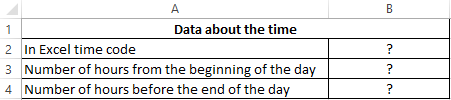
Let’s define the current moment in the Excel time code:

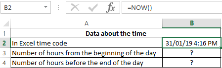
Calculate the number of hours from the beginning of the day:

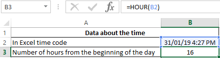
• B2 — the current date and time, expressed in the format Date.

Determine the number of hours before the end of the day:

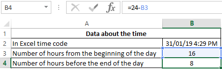
Argument Description:

• 24 — the number of hours per day;
• B3 is the current time in hours, expressed as a numerical value.

Note: The example demonstrates that the result of the work of the HOUR function is a number on which you can perform any arithmetic operation.

Conversion of numbers to time format using the functions HOUR and MINUTE

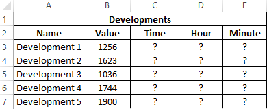
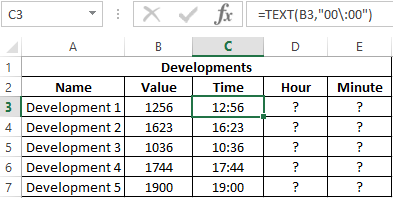
Example 2. From the application, moments of passing certain events that were recognized by Excel as ordinary numbers were loaded (for example, 13:05 was recognized as the number 1305). It is necessary to convert the obtained values into the time format, select the hours and minutes.

Source data table:

To convert the data, use the function:

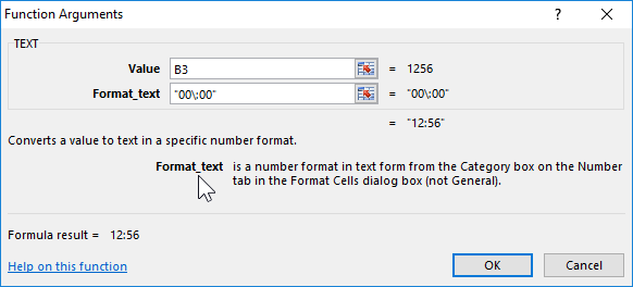
=TEXT(B3,»00:00″)

Argument Description:

• B3 — the value recognized by Excel as a normal number;
• «00:00» is the time format.

As a result, we get:

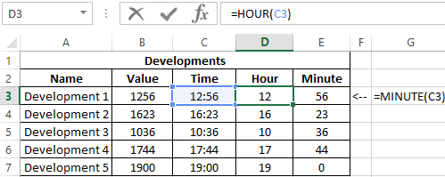
Using the functions HOUR and MINUTE, select the desired values. Similarly, we define the required values for the remaining events:

Example of using the SECOND function in Excel

Example 3. The work day starts at 8:00 am. One worker was systematically late for the previous 10 working days for a few seconds. Determine the total time the employee is late.

Enter the data in the table:

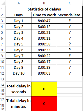
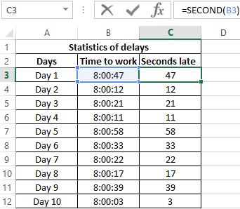
Determine the delay in seconds. Where B3 — data on the time of arrival at work on the first day. Similarly, we define the seconds of delay for the following days:

Determine the total number of seconds of delay:

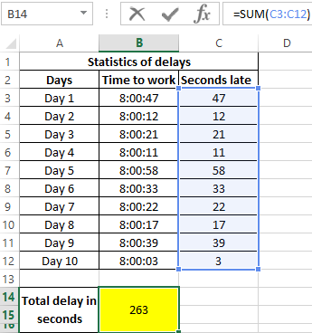
Where C3:C12 is an array of cells containing seconds of late values. We define the integer value of the minutes of delay, knowing that in 1 min = 60 seconds. As a result, we get:

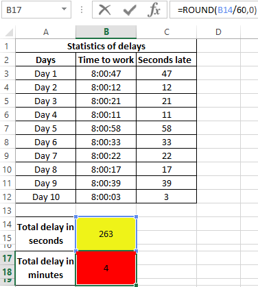
That is, the total lateness of an employee for 10 days was 263 seconds, which is more than 4 minutes.

Features syntax functions HOUR, MINUTE and SECOND in Excel

The HOUR function has the following syntax entry:

=HOUR(serial_number)

• serial_number is the only function argument (required) that characterizes time data that contains data about the clock.

Notes:

1. If a string with text that does not contain time information is passed as an argument to the HOUR function, the error code #VAL! Will be returned.
2. If the logical data type (TRUE, FALSE) or a reference to an empty cell was passed as an argument to the HOUR function, the value 0 will be returned.
3. There are several permitted data formats that the HOUR function accepts:

• In Excel time code (range of values from 0 to 2958465), while the integers correspond to days, fractional — hours, minutes and seconds. For example, 43284.5 is the number of days elapsed between the current moment and the starting point of reference in Excel (01/01/1900 is a conditional date). Fractional part 0.5 corresponds to 12 hours (half of the day).
• In the form of a text string, for example =HOUR(“11:57”). The result of the function — the number 11.
• In the format of the Date and Time Excel. For example, the function will return the values of the clock if, as an argument, it receives a reference to the cell containing the value “07/03/18 11:24” in the date format.
• As a result of the function that returns data in a time format. For example, the function =HOUR(TIMEVALUE(“1:34”)) returns the value 1.

The MINUTE function has the following syntax:

=MINUTE(serial_number)

• serial_number is a required argument describing the value from which the minutes will be calculated.

Notes:

1. As in the case of the HOUR function, the MINUTE function accepts text and numeric data in the format of Dates and Times.
2. If the argument of this function is an empty text string (“”) or a string containing text (“some text”), the error #VALUE! Will be returned.
3. The function supports date format in Excel time code (for example, =MINUTE(0.34) returns the value 9).

The syntax of the SECOND function in Excel is:

=SECOND(serial_number)

• serial_number is the only argument represented as data from which the seconds will be calculated (required for filling).

Download examples HOUR, MINUTE and SECOND to work with time in Excel

Notes:

1. The SECOND function works with text and numeric data types representing Date and Time in Excel.
2. Error #VALUE! will occur in cases where the argument is a text string that does not contain data characterizing the time.
3. The function also calculates seconds from the number represented in the Excel time code (for example, =SECOND(9,567) returns the value 29).