
Today I have a tip for you if you work with very large Excel models. Those, which take minutes or up to hours to calculate. You can calculate selected cells only.
A bit of theory of Excel calculations
Plainly speaking, Excel calculates permanently (with some exceptions) all changed cells and all dependent cells. You can switch the calculation mode to stop calculating in general in-between. This is called “Manual calculation”. Once you have done this, you can
- Recalculate all changed cells by pressing F9 on the keyboard,
- force a full recalculation of all formulas and functions by pressing Ctrl + Alt + F9 on the keyboard or
- only calculate the current worksheet by pressing Shift + F9.
Interest in more theory? In this article you can read more about the calculation modes.
So, what if you only want to recalculate a small amount of cells?
Switch to manual calculation mode first
Before you can use the technique to only calculate smaller parts of your Excel model, you have to switch Excel to manual calculation mode.
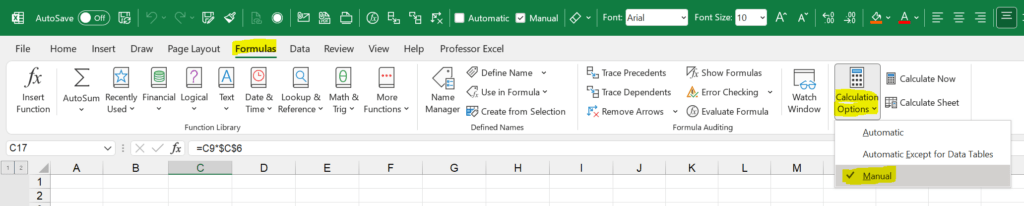
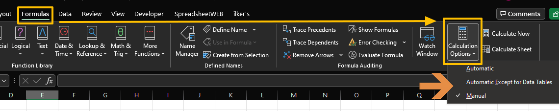
On the Formulas ribbon, go to Calculation Options and make sure that “Manual” is checked.
Please keep in mind: Excel now does not permanently re-calculate. That means, result might not be updated.
Calculate one cell only
Once you are in manual calculation mode it’s quite simple to only calculate one cell:
- Enter the cell you want to recalculation: Select the cell only and press F2 on the keyboard.
- Confirm by pressing Enter on the keyboard.
But what if you don’t want to recalculate one cell only, but rather calculate cells you have currently selected? You basically have two options: Use VBA (it’s simple, no need to insert a module) or use an Excel add-in.
Calculate selected cells by using VBA
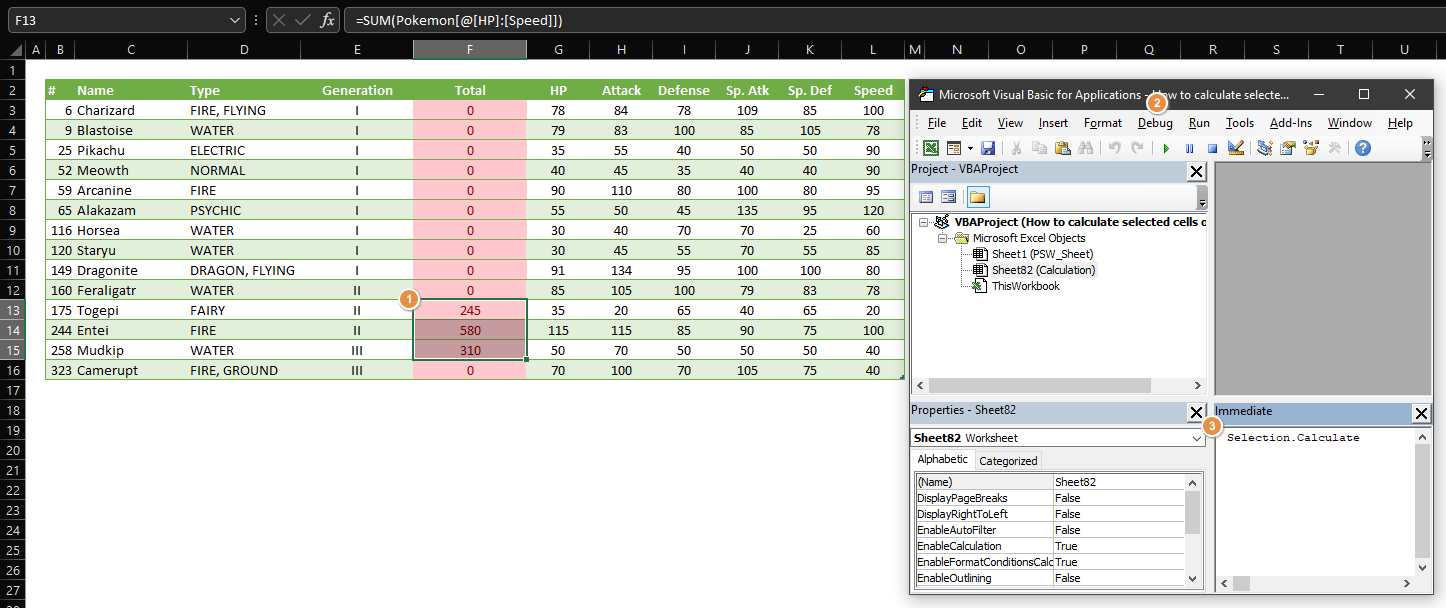
The VBA editor has a feature called “Immediate”. It by default below your code and we can use it here.
- Select the cells you want to calculate.
- Open the VBA editor window by pressing Alt + F11 on the keyboard.
- Type into the Immediate field “Selection.Calculate” and press Enter on the keyboard.
If you want to repeat this, just place the mouse curser at the end of the “Selection.Calculate” and press Enter again.
Calculate selected cells by using an Excel add-in
Our Excel add-in “Professor Excel Tools” comes with more than 120 features. One of them is “Calculate Selection” and can be a real time-saver for you.
Just select the cells you want to calculate and click on “Calculate Selection” on the Professor Excel ribbon.

This function is included in our Excel Add-In ‘Professor Excel Tools’
(No sign-up, download starts directly)
Other advice for such large Excel models
Well, the fact that your Excel model calculates so long might lead to the conclusion that Excel is not the right software for you in this case. So, please consider the following advice:
- Can you use another software (for example PowerBI or any tool / language more suitable, such as Python, R, etc.)?
- Probably, at this point, you have to stay with Excel, right? Then have you considered to use PowerQuery? Could it take over some of the heavier calculation tasks?
- If not, why don’t you take a look at this article of how to speed up Excel or my book “Speeding Up Microsoft Excel“?
Image by Free-Photos from Pixabay

Henrik Schiffner is a freelance business consultant and software developer. He lives and works in Hamburg, Germany. Besides being an Excel enthusiast he loves photography and sports.
Although manual calculation mode helps to deal with big files that take seconds or minutes to be calculated, waiting for the calculation of the entire workbook may not be convenient. Instead, it would be better to calculate certain cells for quick try-error changes. In this guide, we’re going to show you How to calculate selected cells only in Excel.
Download Workbook
Automatic vs. Manual Calculation
As you know, Excel’s default calculation mode is automatic. This means that after each change in your workbook, Excel recalculates all changed cells and all dependent cells as well as volatile functions like OFFSET or INDIRECT. All these recalculations make your system suffer while calculating.
The alternative approach is; manual calculation. When you enable the manual calculation, Excel doesn’t trigger calculations until you or a VBA code gives the command. Thus, you do not wait each time after updating a cell.
You can find the calculation mode in Calculations Options group under Formulas tab.
Once the manual mode is active, you can use either commands from the same section or keyboard shortcuts to trigger the calculations.
| Calculate Now (in Ribbon) | F9 |
| Calculate Sheet (in Ribbon) | Shift + F9 |
| Calculate all worksheets in all workbooks | Ctrl + Alt + F9 |
| Full calculation with dependency tree rebuild | Ctrl + Alt + Shift + F9 |
Data
As an example, we have a column of formulas that should return the sum of the corresponding rows. On the other hand, the manual calculation is enabled in our Excel file and cells still show zero (0) values.

Our intention is to calculate specific cells while others remain as zero.
Calculating Selected Cells
Although it should already be clear, let us warn you beforehand that the calculation setting should be manual. If it is let’s see the approaches.
Single cells
Even in manual calculation mode, if you enter a formula to a cell and press Enter key, Excel will calculate the formula. Thus, there is no turning back if you are entering a new formula into a cell.

Non-VBA Approach
There is a weird technique to calculate the selected cells without VBA. All you need to do is to replace equal signs (=) with equal signs (=). Yes, you read correctly. Excel’s Find & Replace feature allows you to edit multiple cells at once. This way, the previous single-cell trick can be applied to multiple cells. Here are the steps:
- Select the cells you want to calculate.
- Press Ctrl + H to open the Find & Replace
- Enter an equal sign (=) to Find what and Replace with
- Make sure the Within option is Sheet.
- Click Replace All.

- You will see the informational dialog box with updated cells.


VBA Without Macro
Calculating selected cells is a single-line code in the VBA code.
Selection.Calculate
The good thing is that you can run this code in the Immediate Editor and save your workbook as an XLSM file.
- Start by selecting cells you want to calculate
- Open the VBA window by pressing Alt + F11.
- Type or copy-paste the code into the Immediate
- Press Enter key to run.

Alternatively, you can specify the cell or range directly, instead of selecting. Use either Cells or Range objects instead of Selection.
Cells(5,6).Calculate 'F5
Range("F6").Calculate 'F6
[F7:F9].Calculate 'F7:F9
To learn more about referencing ranges in VBA, you can check out How to refer a range or a cell in Excel VBA article.
Macro Approach
Alternatively, you can save the code in a macro and call it via shortcut or a Ribbon command.
- Once the VBA window is open, insert a Module by using the Insert menu in the toolbar.
- Copy&paste the code into the module you created.
- Do not forget to save your file as an XLSM file to keep the macro in it.

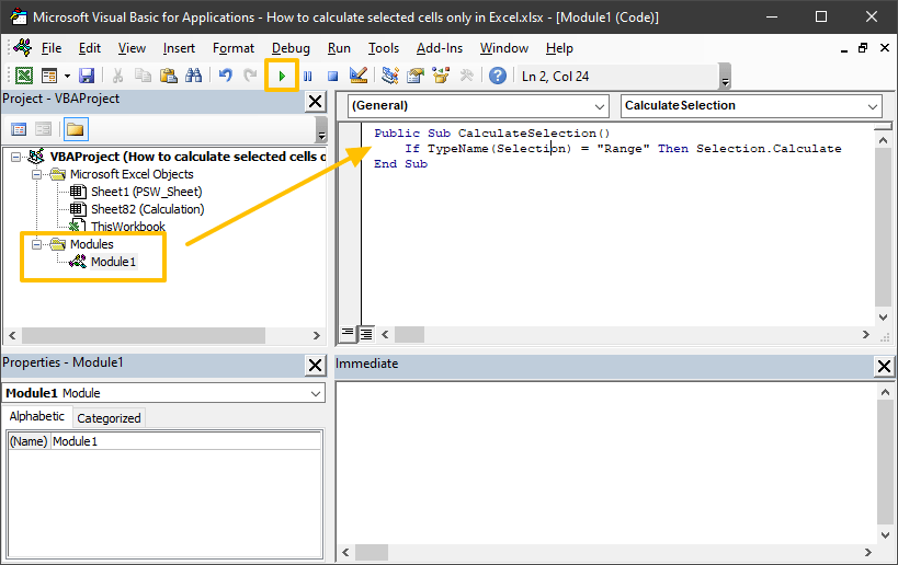
Public Sub CalculateSelection()
    If TypeName(Selection) = "Range" Then Selection.Calculate
End Sub
To run the macro, click inside the macro to see the cursor in the Module window. Then either use the Play button in the toolbar or press F5 key.
Excel is a spreadsheet with a lot of power. The software can be used to track inventory, track and calculate payroll and a myriad of other calculations. An Excel formula is generally composed of several items. Knowing how to calculate formulas in Excel will make tracking various parts of your business that much easier.
Excel Formula Breakdown
Function — This is the desired result. For example, SUM is the function used when you want to add values together.
Cell References — These are the cells that hold the values that are used to complete the function. Example A2, D5, F8, etc.
Arithmetic Operator — This is the operator used to calculate the function. The plus (+), minus (-), multiplication (*) and division (/) symbols are the arithmetic operators.
Constant — the value to which the arithmetic operator is applied. If you are calculating gross pay, the hourly rate is the constant.
Adding Values in Excel
On of the most common uses of Excel is to calculate values. For example, if you’re keeping track of inventory of your office supplies, you add up the total amount of each item by adding the cells together. If Computer Paper takes up Cells C4, C5 and C6, and the total cell is C10, you can add up the values in those cells Use the «=+» formula in the C10 cell. The formula in the C10 cell would look like this:
=+C4+C5+C6
Alternatively, since the cells are consecutive, you could also use the SUM feature to sum multiple columns in Excel, based on criteria. In this instance, you would place the cursor in the C10 cell, then click the SUM key on the Excel toolbar on the formula tab. Then you highlight and drag through keys C4 through C6 and hit Enter. The formula in C10 looks like this:
(SUM=C4:C6).
Calculating Nonadjacent Values in Excel
Even if you have values that are not in an adjacent cell, you can still calculate them. In many cases, there will be values in different parts of a worksheet that have to be calculated together to get the desired results. For example, if you need to use the total number of hours that an employee worked and multiply it by an hourly wage to determine the gross salary, this can be completed, even if the values aren’t side by side. So if the Hours Worked value is in D10 and the Hourly Rate is located in B2, and you want to calculate Gross Pay in F7, the formula you would write in F7 would be =D10*B2.
Examples of Other Calculated Values
Excel has a host of precreated formulas that you can use to complete calculations. These formulas are found on the formula tab on the worksheet. You choose the formula you want to use from the drop-down menu and fill in the cell address for the values you want to use in the formula.
Averages — If you want to know the average of a list of numbers, the formula is =AVERAGE(C4:C6) (using the cells from a previous example. This formula will add the values in C4, C5 and C6 and divide that sum by 3. If there were 15 numbers in the selected area (say C1 through C15) the formula would change to AVERAGE(C1:C15) and the divider would be 15.
If you’re getting started with Excel, creating formulas is one of the first things you should learn. In this lesson you’ll learn how to create simple formulas and calculations in Excel.
At its heart, Excel is a giant calculator. In fact, a simple way to think about Excel is to consider each cell in a worksheet like an individual calculator. An Excel spreadsheet has millions of cells, which means you have millions of individual calculators to work with. Not only that, but you can create formulas that link different cells together (e.g. add the value in this cell to the value in that cell). You can create formulas that link cells in different worksheets together. And you can even create formulas that link cells in different workbooks together.
How to enter a formula in Excel
In Excel, each cell can contain a calculation. In Excel jargon we call this a formula. Each cell can contain one formula. When you enter a formula in a cell, Excel calculates the result of that formula and displays the result of that calculation to you. In fact, when you enter a formula into any cell, Excel will recalculate the result of all the cells in the worksheet. This normally happens in the blink of an eye so you won’t normally notice it, although you may find that large and complex spreadsheets can take longer to recalculate.
When entering a formula, you have to make sure Excel knows that’s what you want to do. You start by typing the = (equals) sign, then the rest of your formula. If you don’t type the equals sign first, then Excel will assume you are typing either a number or a text. You can also start a formula with either a plus (+) or minus (-) symbol. Excel will assume you’re typing a formula and insert the equals sign for you.
Here are some examples of some simple Excel formulas and their results:
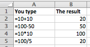
In this example, there are four basic formulas:
- Addition (+)
- Subtraction (—)
- Multiplication (*)
- Division (/)
In each case, you would type the equals sign (=), then the formula, then press Enter to tell Excel you’ve finished.
- Sometimes Excel will show you a warning rather than just entering your formula. This will happen if the formula you’ve typed is invalid, i.e. is not in a format that Excel recognises. It will usually also give you some indication of what you did wrong.
- Other times, Excel may enter the formula you have typed correctly but then show you an error such as #VALUE. This means that you have entered a formula that was value, but Excel could not calculate a valid result from your formula.
Creating formulas that refer to other cells in the same worksheet
Excel’s power comes from allowing you to create formulas that refer to the values in other cells.
In the example above, you’ll notice the headings across the top (A, B) and down the left (1,2,3,4,5). By comining these values, we have a unique reference each cell in a worksheet (A1, A2, A3, B1, B2, B3, and so on).
When you create a formula, you can refer to other cells using these cell references to incorporate the values in other cells into a formula. The value in another cell might be a simple number, or another cell containing a formula. When you create a formula that refers to another cell that also contains a formula, your formula will use the result of the formula in that other cell. Then, if the result of the formula in that other cell changes, so too does the result in your formula.
Here are some examples of some Excel formulas that refer to other cells:
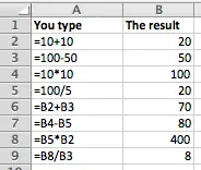
In this example, rows 6-8 build on the earlier examples to link cells together:
- B6 adds the values in B2 and B3 together. If you change either of the values in B2 or B3 the result in B6 will change too.
- B7 and B8 subtract and multiply the values in other cells.
- B9 goes a step further and divides B8 by B3. Note that B8 in turn multiplied B5 and B2 together. So changing the values in either B5 or B2 will have a domino effect, where the value in B8 will change, and so the value in B9 will change too. Note that Excel handles all of this the moment you finish entering a change in either B5 or B2.
Creating formulas that refer to cells in other worksheets
When you first open Excel, you start with a single worksheet. However, Excel allows you to have more than one worksheet inside a single spreadsheet file (known as a workbook). In fact, in earlier versions of Excel a new workbook automatically started out with 3 worksheets inside it.
Earlier we saw how to link two cells together within a worksheet by referring to other cells using their cell reference value. Referring to a cell inside another worksheet works in much the same way, but we need to provide more information about the location of that cell so Excel knows which cell we’re talking about.
Here are some examples of formulas that refer to cells in another worksheet inside the same workbook:
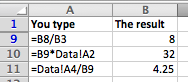
In this example, the formulas in B10 and B11 refer to cells in another worksheet called Data.
- B10 multiples the value in B9 by the value in cell A2 in the worksheet called Data
- B11 takes the value A4 in the worksheet called Data and divides it by the value in B9.
In other words, we’ve told Excel to go to the worksheet called Data and use values in that worksheet in our formulas.
There are a couple of ways to create formulas like this:
- Type the formula in by hand. In the above example, you would create the reference to the other worksheet by typing the worksheet name followed by an exclamation mark (!); the exclamation mark tells Excel that you’re referring to another worksheet.
- Start typing the formula by typing the equals sign (=), then click on the name of the other worksheet. Excel will switch to the other worksheet, and you can click on the cell you want to reference in your formula. You can then press Enter to finish entering the formula, or you can click back on the original worksheet name and finish typing your formula before pressing Enter.
Note that if you rename the worksheet called Data, the formulas that refer to Data will automatically update to reflect the new name. Here’s what the above examples look like if we change the name of the worksheet called Data to Daily Data.
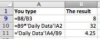
Note how Excel has put apostrophes around the name of the worksheet called Daily Data. This is because of the space in the worksheet name. Excel does this to make sure that the reference still works; if you manually type the formula without the apostrophes then Excel will not be able to validate the formula, and will not let you enter it.
Creating formulas that link to other workbooks
As you might imagine what we’ve already covered, it is also possible to create a formulat that refers to cells in another workbook (i.e. another file). Once again, it’s simply a matter of correctly referring to the cell in the other workbook.
The following example shows what this looks like:
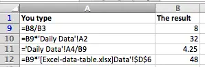
In this example, B12 contains a formula that refers to cell D6 in a worksheet called Data in a file called Excel-data-table-xlsx.
- The square brackets are used to indicate the filename, i.e. [filename]. Be aware that if the file referred to is not currently open, the square brackets may also include the full file path to that file, so that Excel can still read the value from the cell being referred to even though the file is not open.
- The apostrophes are used to enclose the full file name and worksheet name.
- Then, Excel uses absolute references to identify the cell being referred to. This means that if you move (not copy) the contents of cell D6 in the Data worksheet, your formula will still work. The $ signs are used to denote an absolute reference (as opposed to a relative reference). Absolute and relative references are out of scope for this lesson, but you can read about them in this lesson.
Summary
Learning to use Excel formulas is one of the most important things you’ll learn to do with Excel. Hopefully this lesson has set you on the right path, and you’ll be creating spreadsheets with formulas of your own in no time at all. If you have any feedback or questions on this lesson, please comment below!
.
Ready solutions for Excel with the help of formulas working with data spans in the process of complex computations and calculations.
Computing operations with the help of formulas
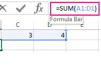 The Formula Bar in Excel, its settings and the purpose.
How to use the formula string and what advantages does it provide for entering and editing data in cells? How to enable or disable the formula bar in the program settings.
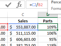 Percentage of the plan implementation by formula in Excel.
The examples of two formulas for calculating of percentages from numbers when analyzing the implementation of sales plans. The example, when and how to use the percentage format of cells.