
The automatic calculator in Excel controls when and how formulas are recalculated.
By default, the auto recalculate Excel feature is always ON, ensuring that any formulas we enter into our worksheet gets recalculated immediately when we open our worksheet or make any changes in names or data sets on which our formulas depend.
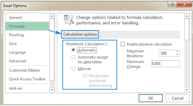 Figure 1. Calculation Options in Excel
To use automatic calculations in Excel efficiently, there are 3 essential considerations that we need to understand;
- Calculation – This is the procedure for computing formulas as well as displaying the resulting values in those cells that contain said formulas.
To prevent unnecessary calculations which can waste our time and reduce the speed of our computer, Microsoft Excel will recalculate formulas automatically only when the data in those cells which the formulas depend on has changed.
This is the go to behavior when we first open our worksheet and when we are editing the worksheet. However, we can regulate when and how automatic recalculation in Excel takes place.
- Iteration – This refers to how worksheets are repeatedly recalculated until a specified numeric condition has been met.
Excel auto calculate cannot work for a formula which refers to the same cell — whether directly or indirectly — that contains our formula. This is known as a “circular reference”.
If our formula is referring back to its own cell(s), we must determine the number of times such formulas should recalculate.
Circular references are able to iterate indefinitely. Still, we can regulate the maximum amount of iterations as well as the frequency of acceptable changes.
- Precision – This refers to the degree of accuracy of an Excel calculation.
Excel calculates and stores with 15 important digits of precision.
Yet, we can regulate the precision of these calculations to ensure that Excel makes use of the displayed values rather than the stored values whenever Excel recalculates formulas.
How to Auto Calculate in Excel
Our worksheet has calculation options that allow us to determine when and how auto calc for Excel formulas takes place.
When we first open/edit our worksheet, the auto calculator in Excel immediately recalculates any formulas whose dependent cell, or formula values have changed.
However, we are free to change this behavior to stop Excel calculations.
To modify Excel calculation options;
- On our worksheet ribbon, click on the “Formulas” tab and then. Under the “Calculation” group, click on “Calculation Options” and select any of the available options:
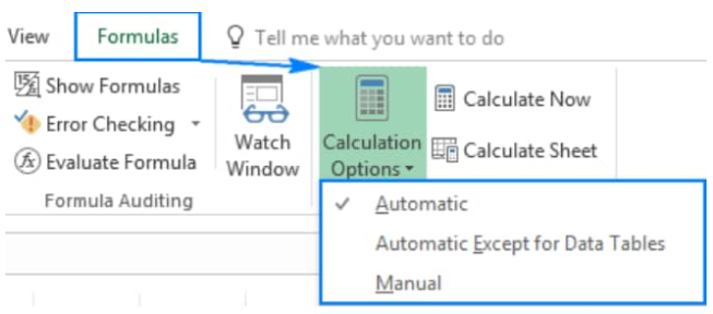 Figure 2. of Calculation Options in Excel
“Automatic” is the default option. It instructs Excel to recalculate any dependent formulas automatically each time any information referenced in our worksheet cells is changed.
The “Automatic Except for Data Tables” option instructs auto calc Excel to automatically recalculate any dependent formulas excluding data tables.
Note however, that this option will turn off calculations in Excel for data tables only, meanwhile the regular Excel table will execute automatic calculations in Excel.
Enabling the “Manual” option will turn off calculations in Excel. Open worksheets will only be recalculated when we force Excel to recalculate.
How to Force Excel to Recalculate
When we open a worksheet and excel is not recalculating our imputed formulas, it most likely means that Excel auto calculate is OFF.
We can either enable the automatic calculator in Excel (see figure 2. above), or force Excel to recalculate.
To recalculate manually, open our worksheet, update all data values, and then click on the “Formulas” tab > “Calculation” group, and then click on the “Calculate Now” button;
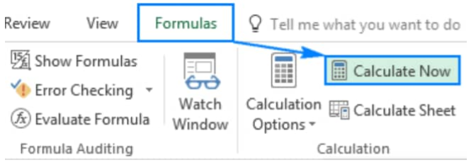 Figure 3. Calculate Now Button in Excel
Instant Connection to an Excel Expert
Most of the time, the problem you will need to solve will be more complex than a simple application of a formula or function. If you want to save hours of research and frustration, try our live Excelchat service! Our Excel Experts are available 24/7 to answer any Excel question you may have. We guarantee a connection within 30 seconds and a customized solution within 20 minutes.
Ready solutions for Excel with the help of formulas working with data spans in the process of complex computations and calculations.
Computing operations with the help of formulas
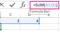 The Formula Bar in Excel, its settings and the purpose.
How to use the formula string and what advantages does it provide for entering and editing data in cells? How to enable or disable the formula bar in the program settings.
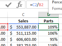 Percentage of the plan implementation by formula in Excel.
The examples of two formulas for calculating of percentages from numbers when analyzing the implementation of sales plans. The example, when and how to use the percentage format of cells.
Does this sound familiar to you: Excel takes too much time calculating. Instead of instantly showing the results, you have to wait for several seconds or even minutes for Excel to finish up the calculation. The problem: The larger your Excel model gets, the more you get frustrated by the lack of performance.
In the previous post, we’ve already described 17 methods of speeding up Excel. Now we are going to have a deeper look at the calculation methods. Switching from automatic calculation mode to manual can save you some time. But the basic question is: When do you want what to be calculated?
The moment of calculating
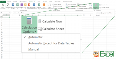
The moment of calculating means, that you can choose between the two basic calculation options ‘Automatic’ and ‘Manual’. The third one (‘Automatic Except for Data Tables’) is similar to ‘Automatic’. Because of that we will now concentrate on the two main options ‘Automatic’ and ‘Manual’.
Automatic calculation calculates after each change
Automatic calculation means, that after each change in your workbook Excel recalculates. Simply speaking, every time you press enter, Excel calculates all the changed cells and the depending cells in your workbook. Also, Excel calculates all volatile functions as INDIRECT or OFFSET. In a small workbook, you won’t notice that, but large workbooks can suffer from performance.
Manual calculation only recalculates when you ask Excel to
Each time, you ask Excel to recalculate. Therefore, go to Formulas. Under Calculation Options you can select Manual (see the image above). Now, Excel will recalculate
- If you actively initiate a recalculation. For example by pressing F9 or by going to Formulas and clicking on Calculate Now (number two on below picture).
- If you save an Excel file, it will also be recalculated. Whereas the first method (pressing F9) can be canceled easily, this method is quite stable.

(Download this and other images as wallpaper to your computer or mobile phone)
When on manual calculation mode, you can (quite roughly though) select, which part of your Excel workbook should be recalculated:
- If you want the whole workbook to be calculated: Switch to manual mode and press F9 or go to Formulas and click on Calculate Now.
- For only calculating the current sheet: In the manual mode, press Shift + F9 or go to Formulas and click on Calculate Sheet.
- If you only press F9, all changes formulas and following cells will be updated. So, when you have the feeling that some formulas aren’t showing correct results, you can force Excel to recalculate the whole workbook by pressing Ctrl + Alt + F9.
- If you only want to calculate a selection of cells/ cell range only, you have to look for a third party solution. We included such function in our Excel add-in ‘Professor Excel Tools’. You can try it for free. There is no sign-up or installation needed, just download and activate it within Excel.
- Besides that, you can decide, if data tables (probably 99% of Excel workbooks don’t have them…) should be recalculated. Go to Formulas, click on Calculation Option and select “Automatic Except for Data Tables”.
Summary
After we’ve taken a look at the different methods, let’s put them together in one table. In the columns we differentiate between ‘Manual’ and ‘Automatic’ calculation.
| What to calculate? | Calculation Mode: Manual | Calculation Mode: Automatic |
|---|---|---|
| All formulas in all open workbooks | Press Ctrl + Shift + F9
|
Press Ctrl + Shift + F9
|
| All changes in all open workbook | Press F9 or go to ‘Formulas’ –> ‘Calculate Now’
|
Not selectable when on automatic mode |
| Worksheet | Press Shift + F9 or go to ‘Formulas’ –> ‘Calculate Sheet’
|
Not selectable when on automatic mode |
| Selection of cells | Go to ‘Professor Excel’ and click on ‘Calculate Selection’ | Not selectable when on automatic mode |
In conclusion, in most situations, you would be fine by remembering these three things:
- If Excel becomes slow, switch to manual calculation mode.
- Recalculate everything by pressing F9.
- Recalculate just the current sheet by pressing Shift + F9.

This function is included in our Excel Add-In ‘Professor Excel Tools’
(No sign-up, download starts directly)

Henrik Schiffner is a freelance business consultant and software developer. He lives and works in Hamburg, Germany. Besides being an Excel enthusiast he loves photography and sports.
If you’re getting started with Excel, creating formulas is one of the first things you should learn. In this lesson you’ll learn how to create simple formulas and calculations in Excel.
At its heart, Excel is a giant calculator. In fact, a simple way to think about Excel is to consider each cell in a worksheet like an individual calculator. An Excel spreadsheet has millions of cells, which means you have millions of individual calculators to work with. Not only that, but you can create formulas that link different cells together (e.g. add the value in this cell to the value in that cell). You can create formulas that link cells in different worksheets together. And you can even create formulas that link cells in different workbooks together.
How to enter a formula in Excel
In Excel, each cell can contain a calculation. In Excel jargon we call this a formula. Each cell can contain one formula. When you enter a formula in a cell, Excel calculates the result of that formula and displays the result of that calculation to you. In fact, when you enter a formula into any cell, Excel will recalculate the result of all the cells in the worksheet. This normally happens in the blink of an eye so you won’t normally notice it, although you may find that large and complex spreadsheets can take longer to recalculate.
When entering a formula, you have to make sure Excel knows that’s what you want to do. You start by typing the = (equals) sign, then the rest of your formula. If you don’t type the equals sign first, then Excel will assume you are typing either a number or a text. You can also start a formula with either a plus (+) or minus (-) symbol. Excel will assume you’re typing a formula and insert the equals sign for you.
Here are some examples of some simple Excel formulas and their results:
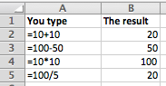
In this example, there are four basic formulas:
- Addition (+)
- Subtraction (—)
- Multiplication (*)
- Division (/)
In each case, you would type the equals sign (=), then the formula, then press Enter to tell Excel you’ve finished.
- Sometimes Excel will show you a warning rather than just entering your formula. This will happen if the formula you’ve typed is invalid, i.e. is not in a format that Excel recognises. It will usually also give you some indication of what you did wrong.
- Other times, Excel may enter the formula you have typed correctly but then show you an error such as #VALUE. This means that you have entered a formula that was value, but Excel could not calculate a valid result from your formula.
Creating formulas that refer to other cells in the same worksheet
Excel’s power comes from allowing you to create formulas that refer to the values in other cells.
In the example above, you’ll notice the headings across the top (A, B) and down the left (1,2,3,4,5). By comining these values, we have a unique reference each cell in a worksheet (A1, A2, A3, B1, B2, B3, and so on).
When you create a formula, you can refer to other cells using these cell references to incorporate the values in other cells into a formula. The value in another cell might be a simple number, or another cell containing a formula. When you create a formula that refers to another cell that also contains a formula, your formula will use the result of the formula in that other cell. Then, if the result of the formula in that other cell changes, so too does the result in your formula.
Here are some examples of some Excel formulas that refer to other cells:
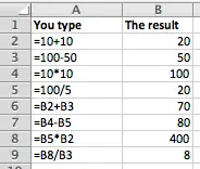
In this example, rows 6-8 build on the earlier examples to link cells together:
- B6 adds the values in B2 and B3 together. If you change either of the values in B2 or B3 the result in B6 will change too.
- B7 and B8 subtract and multiply the values in other cells.
- B9 goes a step further and divides B8 by B3. Note that B8 in turn multiplied B5 and B2 together. So changing the values in either B5 or B2 will have a domino effect, where the value in B8 will change, and so the value in B9 will change too. Note that Excel handles all of this the moment you finish entering a change in either B5 or B2.
Creating formulas that refer to cells in other worksheets
When you first open Excel, you start with a single worksheet. However, Excel allows you to have more than one worksheet inside a single spreadsheet file (known as a workbook). In fact, in earlier versions of Excel a new workbook automatically started out with 3 worksheets inside it.
Earlier we saw how to link two cells together within a worksheet by referring to other cells using their cell reference value. Referring to a cell inside another worksheet works in much the same way, but we need to provide more information about the location of that cell so Excel knows which cell we’re talking about.
Here are some examples of formulas that refer to cells in another worksheet inside the same workbook:
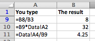
In this example, the formulas in B10 and B11 refer to cells in another worksheet called Data.
- B10 multiples the value in B9 by the value in cell A2 in the worksheet called Data
- B11 takes the value A4 in the worksheet called Data and divides it by the value in B9.
In other words, we’ve told Excel to go to the worksheet called Data and use values in that worksheet in our formulas.
There are a couple of ways to create formulas like this:
- Type the formula in by hand. In the above example, you would create the reference to the other worksheet by typing the worksheet name followed by an exclamation mark (!); the exclamation mark tells Excel that you’re referring to another worksheet.
- Start typing the formula by typing the equals sign (=), then click on the name of the other worksheet. Excel will switch to the other worksheet, and you can click on the cell you want to reference in your formula. You can then press Enter to finish entering the formula, or you can click back on the original worksheet name and finish typing your formula before pressing Enter.
Note that if you rename the worksheet called Data, the formulas that refer to Data will automatically update to reflect the new name. Here’s what the above examples look like if we change the name of the worksheet called Data to Daily Data.
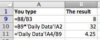
Note how Excel has put apostrophes around the name of the worksheet called Daily Data. This is because of the space in the worksheet name. Excel does this to make sure that the reference still works; if you manually type the formula without the apostrophes then Excel will not be able to validate the formula, and will not let you enter it.
Creating formulas that link to other workbooks
As you might imagine what we’ve already covered, it is also possible to create a formulat that refers to cells in another workbook (i.e. another file). Once again, it’s simply a matter of correctly referring to the cell in the other workbook.
The following example shows what this looks like:
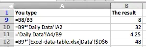
In this example, B12 contains a formula that refers to cell D6 in a worksheet called Data in a file called Excel-data-table-xlsx.
- The square brackets are used to indicate the filename, i.e. [filename]. Be aware that if the file referred to is not currently open, the square brackets may also include the full file path to that file, so that Excel can still read the value from the cell being referred to even though the file is not open.
- The apostrophes are used to enclose the full file name and worksheet name.
- Then, Excel uses absolute references to identify the cell being referred to. This means that if you move (not copy) the contents of cell D6 in the Data worksheet, your formula will still work. The $ signs are used to denote an absolute reference (as opposed to a relative reference). Absolute and relative references are out of scope for this lesson, but you can read about them in this lesson.
Summary
Learning to use Excel formulas is one of the most important things you’ll learn to do with Excel. Hopefully this lesson has set you on the right path, and you’ll be creating spreadsheets with formulas of your own in no time at all. If you have any feedback or questions on this lesson, please comment below!