
![]()
Download Article
![]()
Download Article
Need to find the sum of a column, row, or set of numbers in Excel? Microsoft Excel comes with many mathematical functions, including multiple ways to add sets of numbers. This wikiHow article will teach you the easiest ways to add numbers, cell values, and ranges in Microsoft Excel.
-

1
Click the cell in which you want to display the sum.
-
2
Type an equal sign =. This indicates the beginning of a formula.
Advertisement
-
3
Type the first number you want to add. If you would rather add the value of an existing cell instead of typing a number manually, just click the cell you want to include in the equation. Otherwise, you can type a number manually.
- For example, if you click cell C3, the value of C3 will be the first number in your equation. If you type 1, the number 1 will be the first number in your equation.
-
4
Type a + sign.
-
5
Type another number select another cell. This adds the second number or value to your equation.
- You can add multiple cells or numbers at once if you’d like—just separate each number or address with another + sign.[1]
- For example, if you want to find the sum of cells C3, D4, and E5, your formula will look like this =C3+D4+E5.
- If you want to add 1 plus 1, your formula will look like this: =1+1 .
- You can add other operations, such as subtraction or multiplication, in the same equation. In this example, we’ll add the values of C3 and D4 and then subtract 2: =C3+D4-2
- You can add multiple cells or numbers at once if you’d like—just separate each number or address with another + sign.[1]
-
6
Press ↵ Enter or ⏎ Return. Now you’ll see the sum of the added numbers or values in the selected cell.


Advertisement
-
1
Click the cell in which you want to display the sum. The SUM function works like using the plus + sign, but is a bit easier to work with when you’re adding multiple cells and ranges.
-
2
Type an equal sign followed by the word SUM =SUM. This indicates the beginning of the SUM formula.
-
3
Type an opening parenthesis (. Your formula should now look like this: =SUM(.
-
4
Select the range of cells you want to add. Click and drag over all of the cells you want to add together. For example, if you want to add the values of all cells from A1 through A10, select all of those cells now.
- You can also select multiple columns and rows here. To select multiple non-adjacent columns and/or rows, hold down the Control key and as you select each range.
- You don’t have to select entire ranges with the SUM function—you can also enter individual numbers or cell addresses.
-
5
Type a clothing parenthesis ). This finishes the formula.
- Your formula should now look something like this: =SUM(B4,B8)
- In this example, we’ve selected cells B4 through B8
- If you selected non-adjacent ranges, each range will be separated by a comma. In this example, we selected B4 through C8 (two adjacent columns) and E4 through E5: =SUM(B4:C8,E4:E5)
- Your formula should now look something like this: =SUM(B4,B8)
-
6
Press ↵ Enter or ⏎ Return. The sum of the selected range now appears in this cell.


Advertisement
-
1
Click the cell immediately below or next to the values you want to add. AutoSum will automatically create a formula that adds the values of an adjacent column or row.[2]
- For example, if you want to add the values of cells A:2 through A:10, you would click cell A11.
- You can also add multiple columns or rows at the same time by selecting multiple cells. For example, to display the sums of values in columns A, B, and C, you could select cells A11, B11, and C11.
-
2
Click the AutoSum icon on the Home tab Σ. It’s the Sigma icon (which looks like an «E») on the Home tab at the top of Excel. A formula will then appear in the selected cell.
-
3
Press ↵ Enter or ⏎ Return. Now you’ll see the results of the formula in the cell.
- If you selected multiple blank cells, you’ll see each individual column or row’s value in the selected cells.


Advertisement
Ask a Question
200 characters left
Include your email address to get a message when this question is answered.
Submit
Advertisement
-
Use the SUMIF function to add cells that match certain criteria. For example, if you wanted to find the sum of all cells in A2 through A:10 that are greater than 1, you’d use =SUMIF(A2:A10, ">1").[3]
Thanks for submitting a tip for review!
Advertisement
About This Article
Article SummaryX
1. Use a plus sign to write out formulas like this: =4+5
2. Use the SUM formula to add values from one or more ranges.
3. Use AUTOSUM to automatically find the total of a column or row.
Did this summary help you?
Thanks to all authors for creating a page that has been read 108,680 times.
Is this article up to date?
What are Add-ins in Excel?
An add-ins is an extension that adds more features and options to Microsoft Excel. Providing additional functions to the user increases the power of Excel. An add-in needs to be enabled for usage. Once enabled, it activates as Excel is started.
For example, Excel add-ins can perform tasks like creating, deleting, and updating the data of a workbook. Moreover, one can add buttons to the Excel ribbon and run custom functions with add-ins.
The Solver, Data Analysis (Analysis ToolPakExcel’s data analysis toolpak can be used by users to perform data analysis and other important calculations. It can be manually enabled from the addins section of the files tab by clicking on manage addins, and then checking analysis toolpak.read more), and Analysis ToolPak-VBA are some essential add-ins.
The purposes of activating add-ins are listed as follows: –
- To interact with the objects of Excel
- To avail an extended range of functions and buttons
- To facilitate the setting up of standard add-ins throughout an organization
- To serve the varied needs of a broad audience
In Excel, one can access several Add-ins from “Add-ins” under the “Options” button of the “File” tab. In addition, one can select from the drop-down “Manage” in the “Add-ins” window for more add-ins.
By default, it might hide some add-ins. One can view the unhidden add-ins in the “Data” tab on the Excel ribbonThe ribbon is an element of the UI (User Interface) which is seen as a strip that consists of buttons or tabs; it is available at the top of the excel sheet. This option was first introduced in the Microsoft Excel 2007.read more. For example, it is shown in the following image.
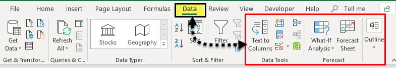
Table of contents
- What are Add-ins in Excel?
- How to Install Add-ins in Excel?
- Types of Add-ins in Excel
- The Data Analysis Add-in
- Create Custom Functions and Install as an Excel Add-in
- Example #1–Extract Comments from the Cells of Excel
- Example #2–Hide Worksheets in Excel
- Example #3–Unhide the Hidden Sheets of Excel
- The Cautions While Creating Add-ins
- Frequently Asked Questions
- Recommended Articles
How to Install Add-ins in Excel?
If Excel is not displaying the add-ins, they need to be installed. The steps to install Excel add-ins are listed as follows:
- First, click on the “File” tab located at the top left corner of Excel.

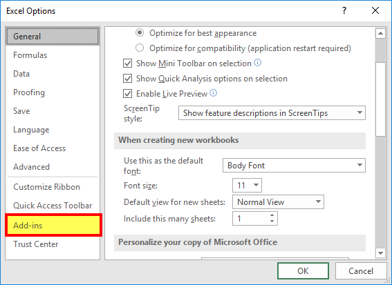
- Click “Options,” as shown in the following image.

- The “Excel Options” window opens. Select “Add-ins.”

- There is a box to the right of “Manage” at the bottom. Click the arrow to view the drop-down menu. Select “Excel add-ins” and click “Go.”

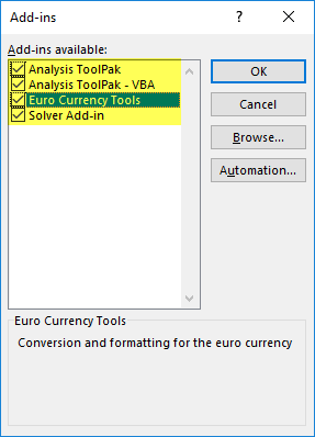
- The “Add-ins” dialog box appears. Select the required checkboxes and click “OK.” We have selected all four add-ins.

- The “Data Analysis” and “Solver” options appear under the “Data tab” of the Excel ribbon.


Types of Add-ins in Excel
The types of add-ins are listed as follows:
- Inbuilt add-ins: These are built into the system. One can unhide them by performing the steps listed under the preceding heading (how to install add-ins in Excel?).
- Downloadable add-ins: These can be downloaded from the Microsoft website (www.office.com).
- Custom add-ins: These are designed to support the basic functionality of Excel. They may be free or chargeable.
The Data Analysis Add-in
The “Data Analysis Tools” pack analyzes statistics, finance, and engineering data.

The various tools available under the “Data Analysis” add-in are shown in the following image.

Create Custom Functions and Install them as an Excel Add-in
Generally, an add-in is created with the help of VBA macrosVBA Macros are the lines of code that instruct the excel to do specific tasks, i.e., once the code is written in Visual Basic Editor (VBE), the user can quickly execute the same task at any time in the workbook. It thus eliminates the repetitive, monotonous tasks and automates the process.read more. Let us learn to create an add-in (in all Excel files) for a custom functionCustom Functions, also known as UDF (User Defined Functions) in Excel, are personalized functions that the users create through VBA programming code to fulfill their particular requirements. read more. For this, first, we make a custom function.
Let us consider some examples.
You can download this Excel Add-Ins Excel Template here – Excel Add-Ins Excel Template
We want to extract comments from specific cells of Excel. Then, create an add-in for the same.
The steps for creating an add-in and extracting comments from cells are listed as follows:
Step 1: Open a new workbook.
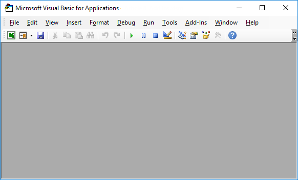
Step 2: Press the shortcutAn Excel shortcut is a technique of performing a manual task in a quicker way.read more “ALT+F11” to access the “Visual Basic Editor.” The following image shows the main screen of Microsoft Visual Basic for Applications.
Step 3: Click “Module” under the “Insert” tab, shown in the following image.

Step 4: Enter the following code in the “module” window.
Function TakeOutComment(CommentCell As Range) As String
TakeOutComment = CommentCell.Comment.Text
End Function

Step 5: Once the code is entered, save the file with the type “Excel add-in.”

Step 6: Open the file containing comments.
Step 7: Select ” Options ” in the “File” tab and select “Options.” Choose “Add-ins.” In the box to the right of “Manage,” select “Excel Add-ins.” Click “Go.”
Click the “Browse” option in the “Add-ins” dialog box.

Step 8: Select the add-in file that had been saved. Click “Ok.”
We saved the file with the name “Excel Add-in.”

Step 9: The workbook’s name (Excel Add-in) that we had saved appears as an add-in, as shown in the following image.
This add-in can be applied as an Excel formula to extract comments.

Step 10: Go to the sheet containing comments. The names of three cities appear with comments, as shown in the following image.

Step 11: In cell B1, enter the symbol “equal to” followed by the function’s name. Type “TakeOutComment,” as shown in the following image.

Step 12: Select cell A1 as the reference. It extracts the comment from the mentioned cell.
Since there are no comments in cells A2 and A3, the formula returns “#VALUE!.”

Example #2–Hide Worksheets in Excel
We want to hide Excel worksheets except for the active sheet. Create an add-in and icon on the Excel toolbar for the same.
The steps to hide worksheets (except for the currently active sheet) and, after that, create an add-in and icon are listed as follows:
Step 1: Open a new workbook.
Step 2: In the “Visual Basic” window, insert a “Module” from the Insert tab. The same is shown in the following image.
Step 3: Copy and paste the following code into the module.
Sub Hide_All_Worksheets_()
Dim As Worksheet
For Each Ws In ActiveWorkbook.Worksheets
If Ws.Name <> ActiveSheet.Name Then
Ws.Visible = xlSheetVeryHidden
End If
Next Ws
End Sub

Step 4: Save this workbook with the type “Excel add-in.”
Step 5: Add this add-in to the new workbook. For this, click “Options” under the “File” tab. Select “Add-ins.” In the box to the right of “Manage,” select “Excel add-in” Click “Go.”
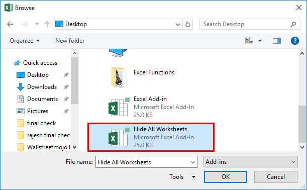
In the “Add-ins” window, choose “Browse.”

Step 6: Select the saved add-in file. Click “Ok.”
We have saved the file with the name “Hide All Worksheets.”
Step 7: The new add-in “Hide All Worksheets” appears in the “Add-ins” window.

Step 8: Right-click the Excel ribbon and select “Customize the Ribbon.”

Step 9: The “Excel Options” window appears. Click “Quick Access Toolbar.” Under the drop-down of “Choose commands from,” select “macrosA macro in excel is a series of instructions in the form of code that helps automate manual tasks, thereby saving time. Excel executes those instructions in a step-by-step manner on the given data. For example, it can be used to automate repetitive tasks such as summation, cell formatting, information copying, etc. thereby rapidly replacing repetitious operations with a few clicks.
read more.”
In the box following this drop-down, choose the name of the macro. Then, click “Add” followed by “OK.” The tasks of this step are shown with the help of black arrows in the following image.
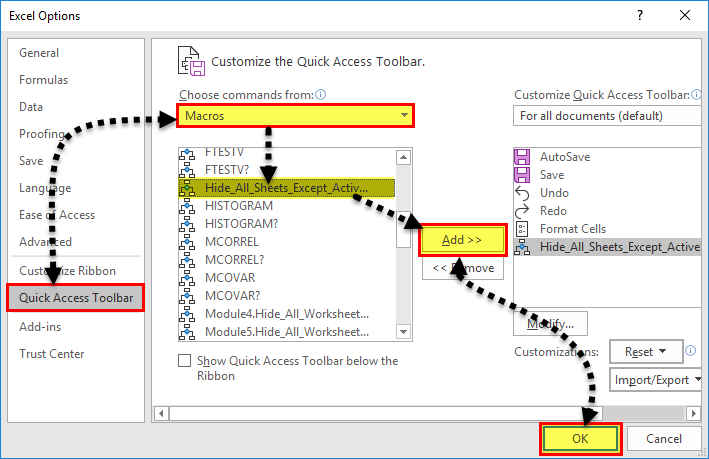
Step 10: A small icon appears on the toolbar. Clicking this icon hides all worksheets except for the currently active sheet.

Example #3–Unhide the Hidden Sheets of Excel
If we want to unhide the sheetsThere are different methods to Unhide Sheets in Excel as per the need to unhide all, all except one, multiple, or a particular worksheet. You can use Right Click, Excel Shortcut Key, or write a VBA code in Excel. read more hidden in the preceding example (example #2). Create an add-in and toolbar icon for the same.
The steps to unhide the sheets and, after that, create an add-in and toolbar icon are listed as follows:
Step 1: Copy and paste the following code to the “Module” inserted in Microsoft Visual Basic for Applications.
Sub UnHide_All_HiddenSheets_()
Dim Ws As Worksheet
For Each Ws In ActiveWorkbook.Worksheets
Ws.Visible = xlSheetVisible
Next Ws
End Sub

Step 2: Save the file as “Excel add-in.” Add this add-in to the sheet.
Right-click the Excel ribbon and choose the option “Customize the ribbon.” Then, in the “Quick Access Toolbar,” select “Macros” under the drop-down of “Choose commands from.”
Choose the macro’s name, click “Add” and “OK.” The tasks of this step are shown with the help of black arrows in the following image.
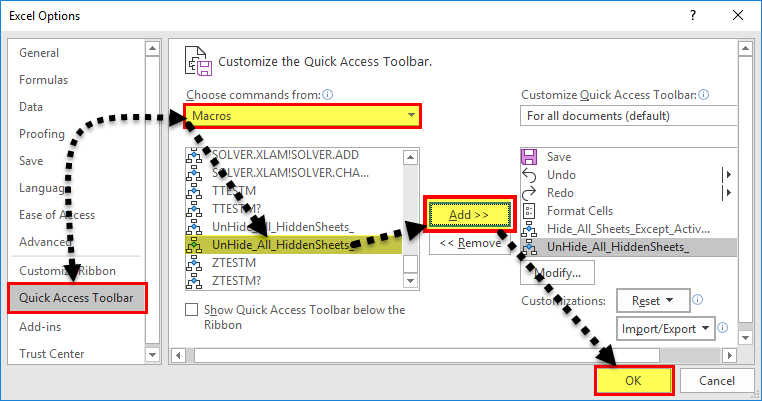
Step 3: Another icon appears on the toolbar. Clicking this icon unhides the hidden worksheets.

The Cautions While Creating Add-ins
The points to be observed while working with add-ins are listed as follows:
- First, remember to save the file in Excel’s “Add-in” extensionExcel extensions represent the file format. It helps the user to save different types of excel files in various formats. For instance, .xlsx is used for simple data, and XLSM is used to store the VBA code.read more of Excel.
- Be careful while selecting the add-ins to be inserted by browsing in the “Add-ins” window.
Note: It is possible to uninstall the unnecessary add-ins at any time.
Frequently Asked Questions
1. What is an add-in? where is it in Excel?
An add-in extends the functions of Excel. It provides more features to the user. It is also possible to create custom functions and insert them as an add-in in Excel.
An add-in can be created, used, and shared with an audience. One can find the add-ins in the “Add-ins” window of Excel.
The steps to access the add-ins in Excel are listed as follows:
a. Click “Options” in the “File” tab of Excel. Select “Add-ins.”
b. In the box to the right of “Manage,” select “Excel add-ins.” Click “Go.”
c. The “Add-ins” window opens. Click “Browse.”
d. Select the required add-in file and click “OK.”
Note: The add-ins already present in the system can be accessed by browsing. Select the corresponding checkbox in the “Add-ins” window and click “OK” to activate an add-in.
2. How to remove an Add-in from Excel?
For removing an add-in from the Excel ribbon, it needs to be inactivated. The steps to inactivate an add-in of Excel are listed as follows:
a. In the File tab, click “Options” and choose “Add-ins”.
b. From the drop-down menu of the “Manage” box, select “Excel add-ins.” Click “Go.”c.
c. In the “Add-ins” window, deselect the checkboxes of the add-ins to be inactivated. Click “OK.”
The deselected add-ins are inactivated. Sometimes, one may need to restart Excel after inactivation. It helps remove the add-in from the ribbon.
Note: Inactivation does not remove an add-in from the computer. For removing an inactivated add-in from the computer, it needs to be uninstalled.
3. How to add an Add-in to the Excel toolbar?
The steps to add an Add-in to the Excel toolbar are listed as follows:
a. In an Excel workbook, press “Alt+F11” to open the Visual Basic Editor. Enter the code by inserting a “module.”
b. Press “Alt+F11” to return to Excel. Save the file as “Excel add-in” (.xlam).
c. In File, select “Options” followed by “Add-ins.” Select “Excel add-ins” in the “Manage” box and click “Go.”
d. Browse this file in the “Add-ins” window. Select the required checkbox and click “OK.”
e. Right-click the ribbon and choose “Customize the Ribbon.” Click “Quick Access Toolbar.”
f. Select “Macros” from the drop-down of “Choose commands from.”
g. Choose the required macro, click “Add” and” OK.”
The icon appears on the toolbar. This icon works in all Excel workbooks as the add-in has been enabled.
Recommended Articles
This article is a step-by-step guide to creating, installing, and using add-ins in Excel. Here, we also discuss the types of Excel add-ins and create a custom function. Take a look at these useful functions of Excel: –
- What is the Quick Access Toolbar in Excel?
- “Save As” Shortcut in Excel
- Remove Duplicates in Excel
- How to Show Formula in Excel?
![]()
You might copy and paste data often in your spreadsheets. But did you know that you can use Excel’s paste feature to perform simple calculations? You can add, subtract, multiply, or divide in a few clicks with paste special in Excel.
Maybe you have prices that you want to increase or costs that you want to decrease by dollar amounts. Or, perhaps you have inventory that you want to increase or decrease by unit amounts. You can perform these types of calculations quickly on a large number of cells simultaneously with Excel’s paste special operations.
For each of the aforementioned calculations, you’ll open the Paste Special dialog box in Excel. So, you’ll start by copying the data and then selecting the cell(s) that you’re pasting to.
To copy, you can press Ctrl+C or right-click and select “Copy.”

Then, do one of the following to access paste special.
- Click the Paste drop-down arrow in the ribbon on the Home tab. Select “Paste Special.”
- Right-click the cells that you’re pasting to and select “Paste Special” in the shortcut menu.
Add, Subtract, Multiply, or Divide Using Paste Special
For basic numbers, decimals, and currency, you can choose from All, Values, or Values and Number Formats in the Paste section of the window. Use the best option for your particular data and formatting.
RELATED: How to Paste Text Without Formatting Almost Anywhere
You’ll then use the section labeled Operation to add, subtract, multiply, or divide.
Let’s look at a simple example of each operation to see how it all works.
Add and Subtract with Paste Special
For this example, we want to add $100 to each of the amounts for our jacket prices to accommodate an increase.
We enter $100 into a cell outside of our data set and copy it. You might already have the data in your sheet or workbook that you need to copy.
Then, we select the cells that we want to add $100 to and access Paste Special as described. We choose “Add” in the Operation section and click “OK.”
And there we go! All of the cells in our selection have increased by $100.
Subtracting an amount works the same way.
Copy the cell containing the amount or number that you want to subtract. For this example, we’re reducing the prices of our jackets by $50.
Select the cells to paste to and open Paste Special. Choose “Subtract” and click “OK.”
Just like with addition, the amount is subtracted from our cells, and we can move on to selling more jackets.
Multiply and Divide with Paste Special
For the multiplication and division examples, we’re going to use numbers instead of currency. Here, we want to quadruple the amount of inventory for our jackets because we received a shipment.
We enter the number 4 into a cell outside of the data set and copy it. Again, you might have the data that you need to copy elsewhere already.
Select the cells to paste to, open Paste Special, select “Multiply,” and click “OK.”
And there we have it! We just quadrupled our numbers in one fell swoop.
For our final example, we need to divide our inventory numbers in half due to missing merchandise. Copy the cell containing the number or amount to divide by. For us, the number is 2.
Select the cells to paste to, open Paste Special, select “Divide,” and click “OK.”
And just like that, our inventory has decreased by half.
Be sure to switch the operation back to “None” when you’re finished.
The next time you need to add, subtract, multiply, or divide a large group of cells in Excel by the same amount, remember this trick using paste special. And for related help, see how to copy and paste in Outlook with attention to formatting.
READ NEXT
- › 12 Basic Excel Functions Everybody Should Know
- › Functions vs. Formulas in Microsoft Excel: What’s the Difference?
- › How to Multiply Columns in Microsoft Excel
- › How to Skip Pasting Blank Cells When Copying in Microsoft Excel
- › Excel for Beginners: The 6 Most Important Tasks to Know
- › 5 Ways to Convert Text to Numbers in Microsoft Excel
- › How to Copy and Paste a Chart From Microsoft Excel
- › BLUETTI Slashed Hundreds off Its Best Power Stations for Easter Sale
You can use Object Linking and Embedding (OLE) to include content from other programs, such as Word or Excel.
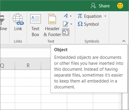
OLE is supported by many different programs, and OLE is used to make content that is created in one program available in another program. For example, you can insert an Office Word document in an Office Excel workbook. To see what types of content that you can insert, click Object in the Text group on the Insert tab. Only programs that are installed on your computer and that support OLE objects appear in the Object type box.
If you copy information between Excel or any program that supports OLE, such as Word, you can copy the information as either a linked object or an embedded object. The main differences between linked objects and embedded objects are where the data is stored and how the object is updated after you place it in the destination file. Embedded objects are stored in the workbook that they are inserted in, and they are not updated. Linked objects remain as separate files, and they can be updated.
Linked and embedded objects in a document
1. An embedded object has no connection to the source file.
2. A linked object is linked to the source file.
3. The source file updates the linked object.
When to use linked objects
If you want the information in your destination file to be updated when the data in the source file changes, use linked objects.
With a linked object, the original information remains stored in the source file. The destination file displays a representation of the linked information but stores only the location of the original data (and the size if the object is an Excel chart object). The source file must remain available on your computer or network to maintain the link to the original data.
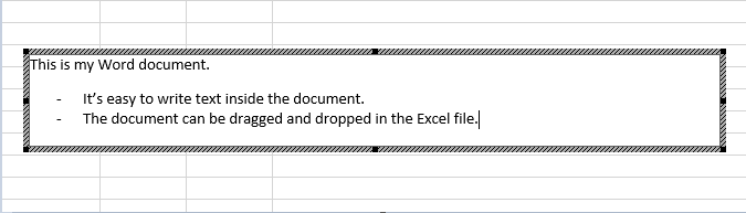
The linked information can be updated automatically if you change the original data in the source file. For example, if you select a paragraph in a Word document and then paste the paragraph as a linked object in an Excel workbook, the information can be updated in Excel if you change the information in your Word document.
When to use embedded objects
If you don’t want to update the copied data when it changes in the source file, use an embedded object. The version of the source is embedded entirely in the workbook. If you copy information as an embedded object, the destination file requires more disk space than if you link the information.
When a user opens the file on another computer, he can view the embedded object without having access to the original data. Because an embedded object has no links to the source file, the object is not updated if you change the original data. To change an embedded object, double-click the object to open and edit it in the source program. The source program (or another program capable of editing the object) must be installed on your computer.
Changing the way that an OLE object is displayed
You can display a linked object or embedded object in a workbook exactly as it appears in the source program or as an icon. If the workbook will be viewed online, and you don’t intend to print the workbook, you can display the object as an icon. This minimizes the amount of display space that the object occupies. Viewers who want to display the information can double-click the icon.
Embed an object in a worksheet
-
Click inside the cell of the spreadsheet where you want to insert the object.
-
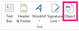
On the Insert tab, in the Text group, click Object
. -
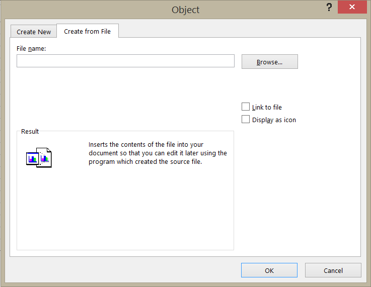
In the Object dialog box, click the Create from File tab.
-
Click Browse, and select the file you want to insert.
-
If you want to insert an icon into the spreadsheet instead of show the contents of the file, select the Display as icon check box. If you don’t select any check boxes, Excel shows the first page of the file. In both cases, the complete file opens with a double click. Click OK.
Note: After you add the icon or file, you can drag and drop it anywhere on the worksheet. You can also resize the icon or file by using the resizing handles. To find the handles, click the file or icon one time.
 .
.
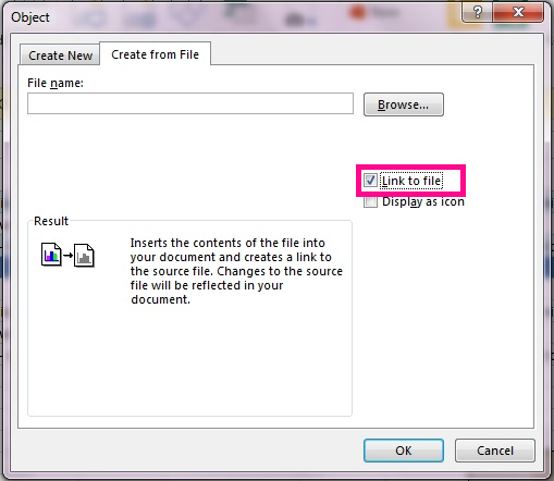
Insert a link to a file
You might want to just add a link to the object rather than fully embedding it. You can do that if your workbook and the object you want to add are both stored on a SharePoint site, a shared network drive, or a similar location, and if the location of the files will remain the same. This is handy if the linked object undergoes changes because the link always opens the most up-to-date document.
Note: If you move the linked file to another location, the link won’t work anymore.
-
Click inside the cell of the spreadsheet where you want to insert the object.
-
On the Insert tab, in the Text group, click Object
. -
Click the Create from File tab.
-
Click Browse, and then select the file you want to link.
-
Select the Link to file check box, and click OK.
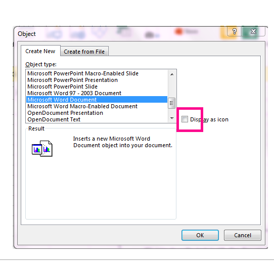
Create a new object from inside Excel
You can create an entirely new object based on another program without leaving your workbook. For example, if you want to add a more detailed explanation to your chart or table, you can create an embedded document, such as a Word or PowerPoint file, in Excel. You can either set your object to be displayed right in a worksheet or add an icon that opens the file.
-
Click inside the cell of the spreadsheet where you want to insert the object.
-
On the Insert tab, in the Text group, click Object
. -
On the Create New tab, select the type of object you want to insert from the list presented. If you want to insert an icon into the spreadsheet instead of the object itself, select the Display as icon check box.
-
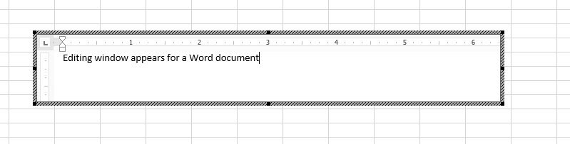
Click OK. Depending on the type of file you are inserting, either a new program window opens or an editing window appears within Excel.
-
Create the new object you want to insert.
When you’re done, if Excel opened a new program window in which you created the object, you can work directly within it.
When you’re done with your work in the window, you can do other tasks without saving the embedded object. When you close the workbook your new objects will be saved automatically.
Note: After you add the object, you can drag and drop it anywhere on your Excel worksheet. You can also resize the object by using the resizing handles. To find the handles, click the object one time.
Embed an object in a worksheet
-
Click inside the cell of the spreadsheet where you want to insert the object.
-
On the Insert tab, in the Text group, click Object.
-
Click the Create from File tab.
-
Click Browse, and select the file you want to insert.
-
If you want to insert an icon into the spreadsheet instead of show the contents of the file, select the Display as icon check box. If you don’t select any check boxes, Excel shows the first page of the file. In both cases, the complete file opens with a double click. Click OK.
Note: After you add the icon or file, you can drag and drop it anywhere on the worksheet. You can also resize the icon or file by using the resizing handles. To find the handles, click the file or icon one time.
Insert a link to a file
You might want to just add a link to the object rather than fully embedding it. You can do that if your workbook and the object you want to add are both stored on a SharePoint site, a shared network drive, or a similar location, and if the location of the files will remain the same. This is handy if the linked object undergoes changes because the link always opens the most up-to-date document.
Note: If you move the linked file to another location, the link won’t work anymore.
-
Click inside the cell of the spreadsheet where you want to insert the object.
-
On the Insert tab, in the Text group, click Object.
-
Click the Create from File tab.
-
Click Browse, and then select the file you want to link.
-
Select the Link to file check box, and click OK.
Create a new object from inside Excel
You can create an entirely new object based on another program without leaving your workbook. For example, if you want to add a more detailed explanation to your chart or table, you can create an embedded document, such as a Word or PowerPoint file, in Excel. You can either set your object to be displayed right in a worksheet or add an icon that opens the file.
-
Click inside the cell of the spreadsheet where you want to insert the object.
-
On the Insert tab, in the Text group, click Object.
-
On the Create New tab, select the type of object you want to insert from the list presented. If you want to insert an icon into the spreadsheet instead of the object itself, select the Display as icon check box.
-
Click OK. Depending on the type of file you are inserting, either a new program window opens or an editing window appears within Excel.
-
Create the new object you want to insert.
When you’re done, if Excel opened a new program window in which you created the object, you can work directly within it.
When you’re done with your work in the window, you can do other tasks without saving the embedded object. When you close the workbook your new objects will be saved automatically.
Note: After you add the object, you can drag and drop it anywhere on your Excel worksheet. You can also resize the object by using the resizing handles. To find the handles, click the object one time.
Link or embed content from another program by using OLE
You can link or embed all or part of the content from another program.
Create a link to content from another program
-
Click in the worksheet where you want to place the linked object.
-
On the Insert tab, in the Text group, click Object.
-
Click the Create from File tab.
-
In the File name box, type the name of the file, or click Browse to select from a list.
-
Select the Link to file check box.
-
Do one of the following:
-
To display the content, clear the Display as icon check box.
-
To display an icon, select the Display as icon check box. Optionally, to change the default icon image or label, click Change Icon, and then click the icon that you want from the Icon list, or type a label in the Caption box.
Note: You cannot use the Object command to insert graphics and certain types of files. To insert a graphic or file, on the Insert tab, in the Illustrations group, click Picture.
-
Embed content from another program
-
Click in the worksheet where you want to place the embedded object.
-
On the Insert tab, in the Text group, click Object.
-
If the document does not already exist, click the Create New tab. In the Object type box, click the type of object that you want to create.
If the document already exists, click the Create from File tab. In the File name box, type the name of the file, or click Browse to select from a list.
-
Clear the Link to file check box.
-
Do one of the following:
-
To display the content, clear the Display as icon check box.
-
To display an icon, select the Display as icon check box. To change the default icon image or label, click Change Icon, and then click the icon that you want from the Icon list, or type a label in the Caption box.
-
Link or embed partial content from another program
-
From a program other than Excel, select the information that you want to copy as a linked or embedded object.
-
On the Home tab, in the Clipboard group, click Copy.
-
Switch to the worksheet that you want to place the information in, and then click where you want the information to appear.
-
On the Home tab, in the Clipboard group, click the arrow below Paste, and then click Paste Special.
-
Do one of the following:
-
To paste the information as a linked object, click Paste link.
-
To paste the information as an embedded object, click Paste. In the As box, click the entry with the word «object» in its name. For example, if you copied the information from a Word document, click Microsoft Word Document Object.
-

Change the way that an OLE object is displayed
-
Right-click the icon or object, point to object typeObject (for example, Document Object), and then click Convert.
-
Do one of the following:
-
To display the content, clear the Display as icon check box.
-
To display an icon, select the Display as icon check box. Optionally, you can change the default icon image or label. To do that, click Change Icon, and then click the icon that you want from the Icon list, or type a label in the Caption box.
-
Control updates to linked objects
You can set links to other programs to be updated in the following ways: automatically, when you open the destination file; manually, when you want to see the previous data before updating with the new data from the source file; or when you specifically request the update, regardless of whether automatic or manual updating is turned on.
Set a link to another program to be updated manually
-
On the Data tab, in the Connections group, click Edit Links.
Note: The Edit Links command is unavailable if your file does not contain links to other files.
-
In the Source list, click the linked object that you want to update. An A in the Update column means that the link is automatic, and an M in the Update column means that the link is set to Manual update.
Tip: To select multiple linked objects, hold down CTRL and click each linked object. To select all linked objects, press CTRL+A.
-
To update a linked object only when you click Update Values, click Manual.
Set a link to another program to be updated automatically
-
On the Data tab, in the Connections group, click Edit Links.
Note: The Edit Links command is unavailable if your file does not contain links to other files.
-
In the Source list, click the linked object that you want to update. An A in the Update column means that the link will update automatically, and an M in the Update column means that the link must be updated manually.
Tip: To select multiple linked objects, hold down CTRL and click each linked object. To select all linked objects, press CTRL+A.
-
Click OK.
Issue: I can’t update the automatic links on my worksheet
The Automatic option can be overridden by the Update links to other documents Excel option.
To ensure that automatic links to OLE objects can be automatically updated:
-
Click the Microsoft Office Button
, click Excel Options, and then click the Advanced category. -
Under When calculating this workbook, make sure that the Update links to other documents check box is selected.
 , click Excel Options, and then click the Advanced category.
Update a link to another program now
-
On the Data tab, in the Connections group, click Edit Links.
Note: The Edit Links command is unavailable if your file does not contain linked information.
-
In the Source list, click the linked object that you want to update.
Tip: To select multiple linked objects, hold down CTRL and click each linked object. To select all linked objects, press CTRL+A.
-
Click Update Values.
Edit content from an OLE program
While you are in Excel, you can change the content linked or embedded from another program.
Edit a linked object in the source program
-
On the Data tab, in the Connections group, click Edit Links.
Note: The Edit Links command is unavailable if your file does not contain linked information.
-
In the Source file list, click the source for the linked object, and then click Open Source.
-
Make the changes that you want to the linked object.
-
Exit the source program to return to the destination file.
Edit an embedded object in the source program
-
Double-click the embedded object to open it.
-
Make the changes that you want to the object.
-
If you are editing the object in place within the open program, click anywhere outside of the object to return to the destination file.
If you edit the embedded object in the source program in a separate window, exit the source program to return to the destination file.
Note: Double-clicking certain embedded objects, such as video and sound clips, plays the object instead of opening a program. To edit one of these embedded objects, right-click the icon or object, point to object typeObject (for example, Media Clip Object), and then click Edit.
Edit an embedded object in a program other than the source program
-
Select the embedded object that you want to edit.
-
Right-click the icon or object, point to object typeObject (for example, Document Object), and then click Convert.
-
Do one of the following:
-
To convert the embedded object to the type that you specify in the list, click Convert to.
-
To open the embedded object as the type that you specify in the list without changing the embedded object type, click Activate.
-
Select an OLE object by using the keyboard
-
Press CTRL+G to display the Go To dialog box.
-
Click Special, select Objects, and then click OK.
-
Press TAB until the object that you want is selected.
-
Press SHIFT+F10.
-
Point to Object or Chart Object, and then click Edit.
Issue: When I double-click a linked or embedded object, a «cannot edit» message appears
This message appears when the source file or source program can’t be opened.
Make sure that the source program is available If the source program is not installed on your computer, convert the object to the file format of a program that you do have installed.
Ensure that memory is adequate Make sure that you have enough memory to run the source program. Close other programs to free up memory, if necessary.
Close all dialog boxes If the source program is running, make sure that it doesn’t have any open dialog boxes. Switch to the source program, and close any open dialog boxes.
Close the source file If the source file is a linked object, make sure that another user doesn’t have it open.
Ensure that the source file name has not changed If the source file that you want to edit is a linked object, make sure that it has the same name as it did when you created the link and that it has not been moved. Select the linked object, and then click the Edit Links command in the Connections group on the Data tab to see the name of the source file. If the source file has been renamed or moved, use the Change Source button in the Edit Links dialog box to locate the source file and reconnect the link.
Need more help?
You can always ask an expert in the Excel Tech Community or get support in the Answers community.
An Excel add-in can be really useful when you have to run a macro often in different workbooks.
For example, suppose you want to highlight all the cells that have an error in it, you can easily create an Excel add-in that will highlight errors with a click of a button.
Something as shown below (the macro has been added to the Quick Access Toolbar to run it with a single click):

Similarly, you may want to create a custom Excel function and use it in all the Excel workbooks, instead of copy pasting the code again and again.
If you’re interested in learning VBA the easy way, check out my Online Excel VBA Training.
Creating an Excel Add-in
In this tutorial, you’ll learn how to create an Excel add-in. There are three steps to create an add-in and make it available in the QAT.
- Write/Record the code in a module.
- Save as an Excel Add-in.
- Add the macro to the Quick Access Toolbar.
Write/Record the Code in a Module
In this example, we will use a simple code to highlight all the cells that have error values:
Sub HighlightErrors()
 Selection.SpecialCells(xlCellTypeFormulas, xlErrors).Select
 Selection.Interior.Color = vbRed
End Sub
If you are writing code (or copy-pasting it from somewhere), here are steps:
Note: If you are recording a macro, Excel automatically takes care of inserting a module and putting the code in it.
Now let’s go ahead and create an add-in out of this code.
Save and Install the Add-in
Follow the below steps when you are in the workbook where you have inserted the code.
Now the add-in has been activated.
You may not see any tab or option appear in the ribbon, but the add-in gets activated at this stage and the code is available to be used now.
The next step is to add the macro to the Quick Access Toolbar so that you can run the macro with a single click.
Note: If you are creating an add-in that has a custom function, then you don’t need to go to step 3. By the end of step 2, you’ll have the function available in all the workbook. Step 3 is for such codes, where you want something to happen when you run the code (such as highlight cells with errors).
Save and Install the Add-in
To do this:
Now to run this code in any workbook, select the dataset and click on the macro icon in the QAT.
This will highlight all the cells with errors in red color. You can also use this macro in any workbook since you have enabled the add-in.
Caution: The changes done by the macro can’t be undone using Control + Z.
You can also create custom functions and then save it as an Excel add-in. Now, when you enable the add-in, the custom functions would be available in all your Excel workbooks.
You May Also Like the Following Excel Tutorials:
- Working with Cells and Ranges in Excel VBA.
- Working with Worksheets in VBA.
- Working with Workbooks in VBA.
- Using Loops in Excel VBA.
- Using IF Then Else Statement in Excel VBA.
- How to Create and Use Personal Macro Workbook in Excel.
- Useful Excel Macro Code Examples.
- Using For Next Loop in Excel VBA.
- Excel VBA Events – An Easy (and Complete) Guide.
- Excel VBA Error Handling