
Excel for Microsoft 365 Excel for Microsoft 365 for Mac Excel for the web Excel 2021 Excel 2021 for Mac Excel 2019 Excel 2019 for Mac Excel 2016 Excel 2016 for Mac Excel 2013 More…Less
We often hear that you want to make data easier to understand by including text in your formulas, such as «2,347 units sold.» To include text in your functions and formulas, surround the text with double quotes («»). The quotes tell Excel it’s dealing with text, and by text, we mean any character, including numbers, spaces, and punctuation. Here’s an example:
=A2&» sold «&B2&» units.»
For this example, pretend the cells in column A contain names, and the cells in column B contain sales numbers. The result would be something like: Buchanan sold 234 units.
The formula uses ampersands (&) to combine the values in columns A and B with the text. Also, notice how the quotes don’t surround cell B2. They enclose the text that comes before and after the cell.
Here’s another example of a common task, adding the date to worksheet. It uses the TEXT and TODAY functions to create a phrase such as «Today is Friday, January 20.»
=»Today is » & TEXT(TODAY(),»dddd, mmmm dd.»)
Let’s see how this one works from the inside out. The TODAY function calculates today’s date, but it displays a number, such as 40679. The TEXT function then converts the number to a readable date by first changing the number to text, and then using «dddd, mmmm dd» to control how the date appears—«Friday, January 20.»
Make sure you surround «ddd, mmmm dd» date format with double quotes, and notice how the format uses commas and spaces. Normally, formulas use commas to separate the arguments—the pieces of data—they need to run. But when you treat commas as text, you can use them whenever you need to.
Finally, the formula uses the & to combine the formatted date with the words «Today is «. And yes, put a space after the «is.»
Need more help?
Excel is a great tool for doing all the analysis and finalizing the report. But sometimes, calculation alone cannot convey the message to the reader because every reader has their way of looking at the report. Some people can understand the numbers just by looking at them, some need some time to get the real story, and some cannot understand. So, they need a full and clear-cut explanation of everything.
You can download this Text in Excel Formula Template here – Text in Excel Formula Template
To bring all the users to the same page while reading the report, we can add text comments to the formula to make the report easily readable.
Let us look at how we can add text in Excel formulas.
Table of contents
- Formula with Text in Excel
- #1 – Add Meaningful Words Using with Text in Excel Formula
- #2 – Add Meaningful Words to Formula Calculations with TIME Format
- #3 – Add Meaningful Words to Formula Calculations with Date Format
- Things to Remember Formula with Text in Excel
- Recommended Articles
#1 – Add Meaningful Words Using Text in Excel Formula
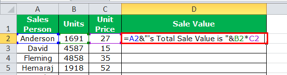
Often in Excel, we only perform calculations. Therefore, we are not worried about how well they convey the message to the reader. For example, take a look at the below data.
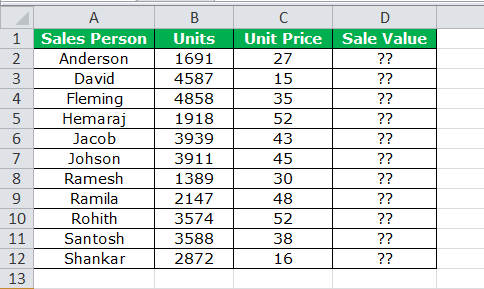
By looking at the above image, it is very clear that we need to find the sale value by multiplying Units to Unit PriceUnit Price is a measurement used for indicating the price of particular goods or services to be exchanged with customers or consumers for money. It includes fixed costs, variable costs, overheads, direct labour, and a profit margin for the organization.read more.
Apply simple text in the Excel formula to get the total sales value for each salesperson.
Usually, we stop the process here itself.
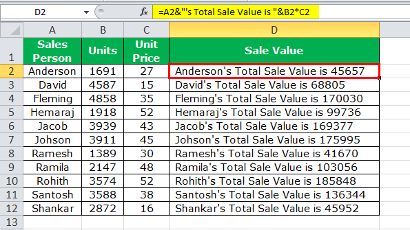
How about showing the calculation as Anderson’s total “Sale Value” is 45,657?
It looks like a complete sentence to convey a clear message to the user. So, let us go ahead and frame a sentence along with the formula.
So, let us go ahead and frame a sentence along with the formula.
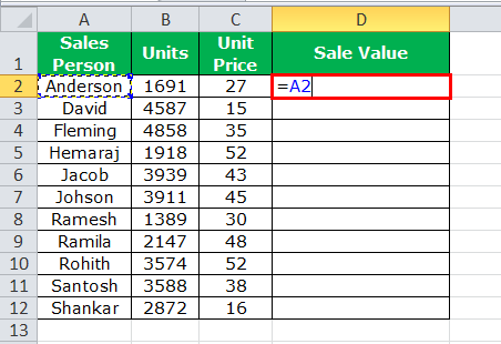
- We know the format of the sentence to be framed. Firstly, we need a “Sales Person” name to appear. So, we must select the cell A2 cell.

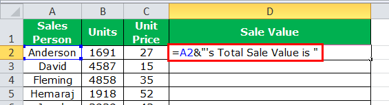
- Now, we need “Total Sale Value” after the salesperson’s name. We need to put the ampersand operator sign after selecting the first cell to comb this text value.

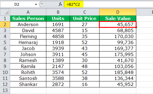
- Now, we need to do the calculation to get the sale value. Put on more (ampersand) sign and apply the formula as B*C2.

- Now, we must press the “Enter” key to complete the formula and our text values.

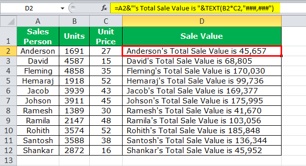
One problem with this formula is that sales numbers are not formatted properly. Because they do not have a thousand separators, that would have made the numbers look properly.
There is nothing to worry about; we can format the numbers with the TEXT function in the Excel formula.
Edit the formula. As shown below, the calculation part applies the Excel TEXT function to format the numbers.

Now, we have the proper format of numbers along with the sales values. The TEXT function in Excel formula format the calculation (B2*C2) to the format of ###, ###.
#2 – Add Meaningful Words to Formula Calculations with TIME Format
We have seen how to add text values to our formulas to convey a clear-cut message to the readers or users. Now, we will be adding text values to another calculation, which includes time calculations.
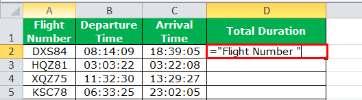
We have data on flight departure and arrival timings. We need to calculate the total duration of each flight.
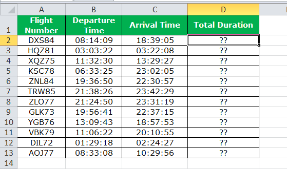
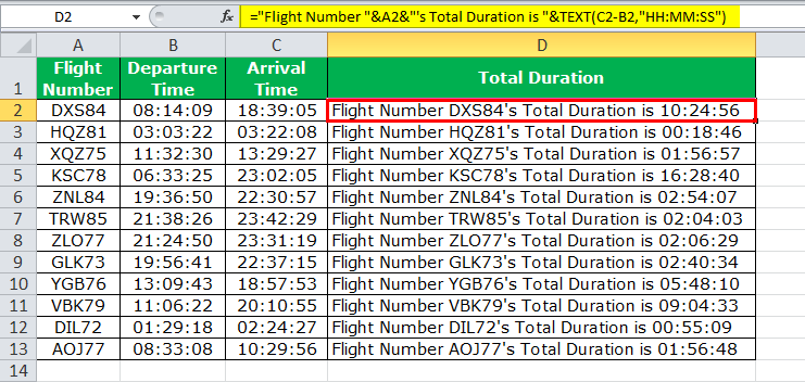
Not only the total duration, but we want to show the message like this “Flight Number DXS84’s total duration is 10:24:56.”
In cell D2, we must start the formula. Our first value is “Flight Number.” We must enter this in double-quotes.
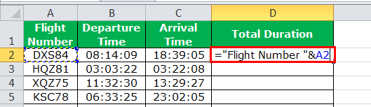
The next value we need to add is the flight number already in cell A2. Enter the “&” symbol and select cell A2.
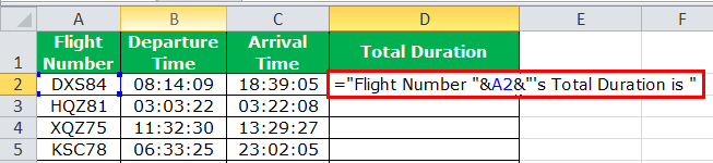
The next thing we need to add to the text‘s “Total Duration.”We must insert one more “&”symbol and enter this text in double-quotes.
Now comes the most important part of the formula. We need to calculate the total duration after “&” the symbol enters the formula as C2 – B2.
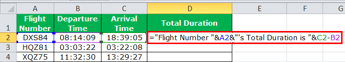
Our full calculation is complete. Press the “Enter” key to get the result.
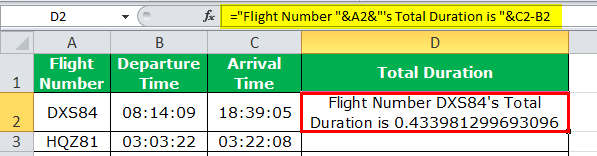
We got the total duration as 0.433398, which is not in the right format. So, we must apply the TEXT function to perform the calculation and format that to TIME.
#3 – Add Meaningful Words to Formula Calculations with Date Format
The TEXT function can perform the formatting task when adding text values to get the correct number format. Now, we will see it in the date format.
Below is the daily sales table that we update the values regularly.
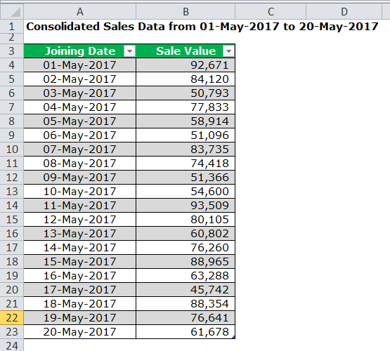
We need to automate the heading as the data keeps adding, i.e., we should change the last date as per the last day of the table.
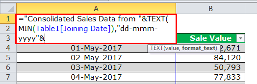
Step 1: We must first open the formula in the A1 cell as “Consolidated Sales Data from.”
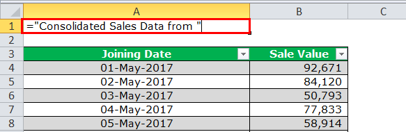
Step 2: Put the “&” symbol and apply the TEXT function in the Excel formula. Apply the MIN function to get the least date from this list inside the TEXT function. And format it as “dd-mmm-yyyy.”
Step 3: Now, enter the word to.
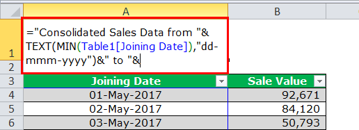
Step 4: To get the latest date from the table, we must apply the MAX formulaThe MAX Formula in Excel is used to calculate the maximum value from a set of data/array. It counts numbers but ignores empty cells, text, the logical values TRUE and FALSE, and text values.read more, and format it as the date by using TEXT in the Excel formula.
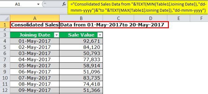
As we update the table, it will automatically update the heading.
Things to Remember Formula with Text in Excel
- We can add the text values according to our preferences by using the CONCATENATE function in excelThe CONCATENATE function in Excel helps the user concatenate or join two or more cell values which may be in the form of characters, strings or numbers.read more or the ampersand (&) symbol.
- To get the correct number format, we must use the TEXT function and specify the number format we want to display.
Recommended Articles
This article has been a guide on Text in Excel Formula. Here, we discuss how to add text in the Excel formula cell along with practical examples and downloadable Excel templates. You may also look at these useful functions in Excel: –
- Separate Text in Excel
- How to Wrap Text in Excel?
- How to Convert Text to Numbers in Excel?
- Convert Date to Text in Excel
There may be instances where you need to add the same text to all cells in a column. You might need to add a particular title before names in a list, or a particular symbol at the end of the text in every cell.
The good thing is you don’t need to do this manually.
Excel provides some really simple ways in which you can add text to the beginning and/ or end of the text in a range of cells.
In this tutorial we will see 4 ways to do this:
- Using the ampersand operator (&)
- Using the CONCATENATE function
- Using the Flash Fill feature
- Using VBA
So let’s get started!
Method 1: Using the ampersand Operator
An ampersand (&) can be used to easily combine text strings in Excel. Let’s see how you use it to add text at the beginning or end or both in Excel.
Using the ampersand Operator to Add Text to the Beginning of all Cells
The ampersand (&) is an operator that is mainly used to join several text strings into one.
Here’s how you can use it to add text to the beginning of all cells in a range. Let us assume you have the following list of names and want to add the title “Prof.” before every name:

Below are the steps to add a text before a text string in Excel:
- Click on the first cell of the column where you want the converted names to appear (B2).
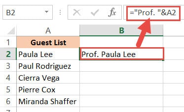
- Type equal sign (=), followed by the text “Prof. “, followed by an ampersand (&).
- Select the cell containing the first name (A2).
- Press the Return Key.
- You will notice that the title “Prof.” is added before the first name in the list.

- It’s now time to copy this formula to the rest of the cells in the column. Simply double click the fill handle (located at the bottom right of cell B2). Alternatively, you can drag down the fill handle to achieve the same effect.
That’s it, all your cells in column B should now contain the title “Prof.” preceding each name.

Using the ampersand Operator to Add Text to the End of all Cells
Now let us see how to add some text to the end of every name in the dataset. Let us say you want to add the text “(MD)” at the end of every name. In that case, here are the steps you need to follow:
- Click on the first cell of the column where you want the converted names to appear (C2 in our case).
- Type equal sign (=)
- Select the cell containing the first name (B2 in our case).
- Next, insert an ampersand (&), followed by the text “ (MD)”.
- Press the Return Key.
- You will notice that the text “(MD).” added after the first name in the list.

- It’s now time to copy this formula to the rest of the cells in the column. Simply double click the fill handle (located at the bottom right of cell C2). Alternatively, you can drag down the fill handle to achieve the same effect.

All your cells in column C should now contain the text “(MD”) at the end of each name.

Method 2: Using the CONCATENATE Function
CONCATENATE is an Excel function that you can use to add text at the beginning and end of the text string.
Let’s see how to use CONCATENATE to do this.
Using CONCATENATE to Add Text to the Beginning of all Cells
The CONCATENATE() function provides the same functionality as the ampersand (&) operator. The only difference is in the way both are used.
The general syntax for the CONCATENATE function is:
=CONCATENATE(text1, [text2], …)
Where text1, text2, etc. are substrings that you want to combine together.
Let’s apply the CONCATENATE function to the same dataset as above:
- Click on the first cell of the column where you want the converted names to appear (B2).
- Type equal sign (=).
- Enter the function CONCATENATE, followed by an opening bracket (.
- Type the title “Prof. ” in double-quotes, followed by a comma (,).
- Select the cell containing the first name (A2)
- Place a closing bracket. In our example, your formula should now be: =CONCATENATE(“Prof. “,A2).
- Press the Return Key.
- You will notice that the title “Prof.” is added before the first name on the list.

- It’s now time to copy this formula to the rest of the cells in the column. Simply double click the fill handle (located at the bottom right of cell B2). Alternatively, you can drag down the fill handle to achieve the same effect.

That’s it, all your cells in column B should now contain the title “Prof.” preceding each name.

Using CONCATENATE to Add Text to the End of all Cells
Now let us see how to add some text to the end of every name in the dataset. Let us say you want to add the text “(MD)” at the end of every name. In that case, here are the steps you need to follow:
- Click on the first cell of the column where you want the converted names to appear (C2 in our example).
- Type equal sign (=).
- Enter the function CONCATENATE, followed by an opening bracket (.
- Select the cell containing the first name (B2 in our example).
- Next, insert a comma, followed by the text “ (MD)”.
- Place a closing bracket. In our example, your formula should now be: =CONCATENATE(B2,” (MD)”).
- Press the Return Key.
- You will notice that the text “(MD).” added after the first name in the list.

- It’s now time to copy this formula to the rest of the cells in the column. Simply double click the fill handle (located at the bottom right of cell C2).

All your cells in column C should now contain the text “(MD”) at the end of each name.

Notice that since you’re using a formula, your column C depends on columns A and B. So if you make any changes to the original values in column A, they get reflected in column C.
If you decide to only retain the converted names and delete columns A and B, you will get an error, as shown below:

To make sure that this does not happen, it’s best to first convert the formula results to permanent values copying them and pasting them as values in the same column (Right-click and select Paste Options->Values from the Popup menu).

Now you can go ahead and delete columns A and B if you need to.
Also read: How to Remove First Character in Excel?
Method 3: Using the Flash Fill Feature
Flash fill is a relatively new feature that looks at the pattern of what you are trying to achieve and then does it for all the cells in a column.
You can also use Flash fill to so text manipulation as we will see in the following examples.
Using Flash Fill to Add Text to the Beginning of all Cells
The Excel flash fill feature is like a magical button. It is available if you’re on any Excel version from 2013 onwards.
The feature takes advantage of Excel’s pattern recognition capabilities. It basically recognizes a pattern in your data and automatically fills in the other cells of the column with the same pattern for you.
Here’s how you can use Flash Fill to add text to the beginning of all cells in a column:
- Click on the first cell of the column where you want the converted names to appear (B2).
- Manually type in the text Prof. , followed by the first name of your list.

- Press the Return Key.
- Click on cell B2 again.
- Under the Data tab, click on the Flash Fill button (in the ‘Data Tools’ group). Alternatively, you can just press CTRL+E on your keyboard (Command+E if you’re on a Mac).


This will copy the same pattern to the rest of the cells in the column… in a flash!

Using Flash Fill to Add Text to the End of all Cells in a Column
If you want to add the text “ (MD)” to the end of the names, follow the same steps:
- Click on the first cell of the column where you want the converted names to appear (C2).
- Manually type in or copy the text from column B2 into C2.
- Add the text “(MD)” after that.

- Under the Data tab, click on the Flash Fill or press CTRL+E on your keyboard (Command+E if you’re on a Mac).

That’s all, you get every cell filled in with the same pattern!

We especially like this method because it is simple, quick, and easy. Moreover, since it’s formula-free, the results do not depend on the original columns.
So they remain unchanged even if you delete rows A and B!

Method 4: Using VBA Code
And of course, if you’re comfortable with VBA, you can also add text before or after a text string using it.
Using VBA to Add Text to the Beginning of all Cells in a Column
If coding with VBA does not intimidate you then this method can help get your work done quickly too.
Here’s the code we will be using to add the title “Prof. “ to the beginning of all cells in a range. You can select and copy it:
Sub add_text_to_beginning()
Dim rng As Range
Dim cell As Range
Set rng = Application.Selection
For Each cell In rng
cell.Offset(0, 1).Value = "Prof. " & cell.Value
Next cell
End Sub
Follow these steps to use the above code:
- From the Developer Menu Ribbon, select Visual Basic.
- Once your VBA window opens, Click Insert->Module. Now you can start coding. Type or copy-paste the above lines of code into the module window. Your code is now ready to run.
- Select the range of cells containing the text you want to convert. Make sure the column next to it is blank because this is where the code will display the results.
- Navigate to Developer->Macros-> add_text_to_beginning->Run.
You will now see the converted text next to your selected range of cells.
Note: You can change the text in line 6 from “Prof. ” to whatever text you need to add to the beginning of all cells.
Using VBA to Add Text to the End of all Cells in a Column
Now, what if you want to add text to the end of all the cells, instead of the beginning? This only involves making a tweak to line 6 of the above code. So if you want to add the text “ (MD)” to the end of all cells, change line 6 to:
cell.Offset(0, 1).Value = cell.Value & “ (MD)”
So your full code should now be:
Sub add_text_to_end()
Dim rng As Range
Dim cell As Range
Set rng = Application.Selection
For Each cell In rng
cell.Offset(0, 1).Value = cell.Value & " (MD)"
Next cell
End Sub
Here’s the final result:
You can now delete the first two columns if you need to. Do remember to keep a backup of your sheet, because the results of VBA code are usually irreversible.
Note: You can change the text in line 6 from “ (MD)” to whatever text you need to add to the end of all cells in the range.
In this tutorial, we showed you four ways in which you can add text to the beginning and/ or end of all cells in a range.
There are plenty of other methods that you can find online too, and all of them work just as well as the ones shown here.
You may feel free to choose whatever method suits you, your requirement, and your version of Excel. In the end, what matters is getting what you need to be done quickly and effectively.
Other Excel tutorials you may like:
- How to Remove Text after a Specific Character in Excel
- How to Reverse a Text String in Excel
- How to Count How Many Times a Word Appears in Excel
- How to Remove Commas in Excel (from Numbers or Text String)
- How to Remove a Specific Character from a String in Excel
- How to Change Uppercase to Lowercase in Excel
- How to Separate Address in Excel?
- How to Concatenate with Line Breaks in Excel?
- How to Separate Names in Excel
This post explains that how to add the specified text or characters to the beginning of all cells in excel. How to create an excel formula to add same text string or characters to the beginning of text string in one Cell. How to create an excel macro to add specific text to the beginning of the text in all of cells.
Table of Contents
- Add text to the beginning of all cells with Formula
- Add text to the beginning of all cells with Excel VBA
- Related Formulas
- Related Functions
If you want to add the specific text or characters into the beginning of the text in one cell or all cells, you can create an excel formula based on the concatenate operator or CONCATENATE function.
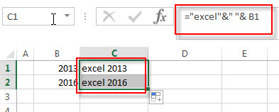
Assuming that you want to add text “excel” into the beginning of the text in Cell B1, you can write down the following formula:
="excel"&" "& B2
OR
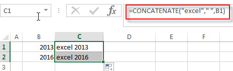
=CONCATENATE(“excel”,””,B1)
You can enter the above formulas in Cell C1, and then drag the fill handle down to other cells in column C and you will see that the specific text will add the beginning of the text in Cell B1.
Add text to the beginning of all cells with Excel VBA
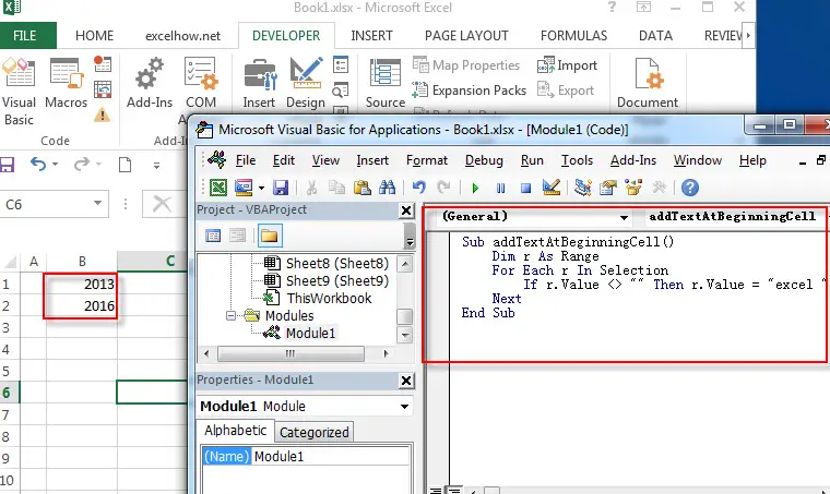
You can create a new excel macro to add text string “excel” to the beginning of text in Cell B1 in Excel VBA, just refer to the below steps:
1# click on “Visual Basic” command under DEVELOPER Tab.

2# then the “Visual Basic Editor” window will appear.
3# click “Insert” ->”Module” to create a new module

4# paste the below VBA code into the code window. Then clicking “Save” button.
Sub addTextAtBeginningCell()
    Dim r As Range
    For Each r In Selection
        If r.Value <> "" Then r.Value = "excel " & r.Value
    Next
End Sub
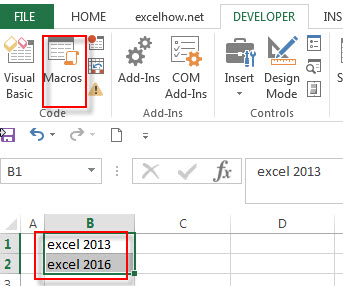
5# back to the current worksheet, then run the above excel macro, you will see that the specific text “excel” has been added into the beginning of the text in all selected Cells.
- How to add text to the end all cells
To add the specified text string or characters to the end of all selected cells in excel, you can use the concatenate operator or the CONCATENATE function to create an excel formula..… - How to join text from two or more cells into one cell separated by commas, space
You can merge text from two or more cells into one cell using a combination of the SUBSTITUTE function, the TRIM function and concatenation operator to create an excel formula..… - Combine columns without losing data
How to keep all data after merging columns. You can use the concatenate operator or CONCATENATE function to create an excel formula. Assuming that you want to merge column B and C into column D, you can use the following formulas:=B2&C2 OR =CONCATENATE(B2, “ “ ,C2).… - How to Extract Text between Commas
To extract text between commas in Cell B1, you can use the following formula based on the SUBSTITUTE function, the MID function and the REPT function.… - How to Combine Text from Two or More Cells into One Cell
If you want to join the text from multiple cells into one cell, you also can use the CONCATENATE function instead of Ampersand operator..…
- Excel Concat function
The excel CONCAT function combines 2 or more strings or ranges together.This is a new function in Excel 2016 and it replaces the CONCATENATE function.The syntax of the CONCAT function is as below:=CONCAT (text1,[text2],…)…
Содержание
- How to add text to beginning or end of all cells in Excel
- The CONCAT and CONCATENATE Function
- Adding Text Using Ampersand Operator ( &)
- How to Add Text to the Beginning or End of all Cells in Excel
- Method 1: Using the ampersand Operator
- Using the ampersand Operator to Add Text to the Beginning of all Cells
- Using the ampersand Operator to Add Text to the End of all Cells
- Method 2: Using the CONCATENATE Function
- Using CONCATENATE to Add Text to the Beginning of all Cells
- Using CONCATENATE to Add Text to the End of all Cells
- Method 3: Using the Flash Fill Feature
- Using Flash Fill to Add Text to the Beginning of all Cells
- Using Flash Fill to Add Text to the End of all Cells in a Column
- Method 4: Using VBA Code
- Using VBA to Add Text to the Beginning of all Cells in a Column
- Using VBA to Add Text to the End of all Cells in a Column
How to add text to beginning or end of all cells in Excel
A free Office suite fully compatible with Microsoft Office
A free Office suite fully compatible with Microsoft Office
In order to make sure that the data in your Excel file is organized in a way that makes sense, you will want to add some text to the beginning or end of all cells. This is not just for aesthetic purposes—it’s also important because it will help you keep track of what the data means.
In some cases, you may need to add text to the beginning of all cells in Excel. For example, if you have a list of addresses and you want to include each address with its corresponding city name, then adding Address or City to the beginning of all cells will be useful.
Information provided in this article are compatible with versions 2010/2016/MAC/online.
The CONCAT and CONCATENATE Function
CONCAT AND CONCATENATE function are very helpful if you wish to add a certain title in the beginning or end of a list. Here, I will show you an example of adding “Dr.” to the beginning of a list of names.
1. Type “=con” in the target cell and choose if you want to use the CONCAT or the CONCATENATE function. Double-click on the chosen function.
2. Type the argument as the text you want to add in inverted commas (“”) and choose the cell you wish to add after it.
4. It’s time to duplicate this formula in the remaining column’s cells. Just click twice on the fill handle or hold and drag it down (located at the bottom right of cell the here B2).
5. You can see that it adds the prefix you want to add to all the cells, as far as you drag down.
6. Alternatively, Ctrl+C (copy) and Ctrl+V (paste) on keyboard can be used for shorter lists, that is copying and pasting the formula onto other cells.
Adding Text Using Ampersand Operator ( &)
1.The & operator can also be used to add text in the beginning or end of many cells. Let’s discuss an example where you need to add the percentage sybol (%) after a lot of numbers.
2. Just type in “=” and the formula as shown.
3. The result would look like this when you press enter.
4. If you want a space between the number and the symbol, you can go about two following ways:
5. Note that the space is added before the symbol.
6. To duplicate this formula in the remaining column’s cells, just click twice on the fill handle at the bottom-right corner of each cell or hold and drag it down. Or use Ctrl+C (copy) and Ctrl+V (paste) on keyboard for shorter lists.
The Flash Fill Option
1.If you wish to fill many cells with the same prefix, the Flash fill option can be very useful.
2. Under the ‘Data’ option in the main menu, a ‘Fill’ drop-down menu is availabele that has the ‘Flash Fill’ option.
3. Click on the text you want to fill onto the other cells and click on the Flash Fill option. The data will be copied onto the other cells related to the data. A shortcut of Flash Fill is Ctrl+E on keyboard.
Did you learn about How To Add Text To Beginning Or End Of All Cells In Excel? You can follow WPS Academy to learn more features of Word Document, Excel Spreadsheets and PowerPoint Slides.
You can also download WPS Office to edit the word documents, excel, PowerPoint for free of cost. Download now! And get an easy and enjoyable working experience.
Источник
How to Add Text to the Beginning or End of all Cells in Excel
There may be instances where you need to add the same text to all cells in a column. You might need to add a particular title before names in a list, or a particular symbol at the end of the text in every cell.
The good thing is you don’t need to do this manually.
Excel provides some really simple ways in which you can add text to the beginning and/ or end of the text in a range of cells.
In this tutorial we will see 4 ways to do this:
- Using the ampersand operator (&)
- Using the CONCATENATE function
- Using the Flash Fill feature
- Using VBA
So let’s get started!
Table of Contents
Method 1: Using the ampersand Operator
An ampersand (&) can be used to easily combine text strings in Excel. Let’s see how you use it to add text at the beginning or end or both in Excel.
Using the ampersand Operator to Add Text to the Beginning of all Cells
The ampersand (&) is an operator that is mainly used to join several text strings into one.
Here’s how you can use it to add text to the beginning of all cells in a range. Let us assume you have the following list of names and want to add the title “Prof.” before every name:
Below are the steps to add a text before a text string in Excel:
- Click on the first cell of the column where you want the converted names to appear (B2).
- Type equal sign (=), followed by the text “Prof. “, followed by an ampersand (&).
- Select the cell containing the first name (A2).
- Press the Return Key.
- You will notice that the title “Prof.” is added before the first name in the list.

- It’s now time to copy this formula to the rest of the cells in the column. Simply double click the fill handle (located at the bottom right of cell B2). Alternatively, you can drag down the fill handle to achieve the same effect.
That’s it, all your cells in column B should now contain the title “Prof.” preceding each name.
Using the ampersand Operator to Add Text to the End of all Cells
Now let us see how to add some text to the end of every name in the dataset. Let us say you want to add the text “(MD)” at the end of every name. In that case, here are the steps you need to follow:
- Click on the first cell of the column where you want the converted names to appear (C2 in our case).
- Type equal sign (=)
- Select the cell containing the first name (B2 in our case).
- Next, insert an ampersand (&), followed by the text “ (MD)”.
- Press the Return Key.
- You will notice that the text “(MD).” added after the first name in the list.
- It’s now time to copy this formula to the rest of the cells in the column. Simply double click the fill handle (located at the bottom right of cell C2). Alternatively, you can drag down the fill handle to achieve the same effect.
All your cells in column C should now contain the text “(MD”) at the end of each name.
Method 2: Using the CONCATENATE Function
CONCATENATE is an Excel function that you can use to add text at the beginning and end of the text string.
Let’s see how to use CONCATENATE to do this.
Using CONCATENATE to Add Text to the Beginning of all Cells
The CONCATENATE() function provides the same functionality as the ampersand (&) operator. The only difference is in the way both are used.
The general syntax for the CONCATENATE function is:
Where text1, text2, etc. are substrings that you want to combine together.
Let’s apply the CONCATENATE function to the same dataset as above:
- Click on the first cell of the column where you want the converted names to appear (B2).
- Type equal sign (=).
- Enter the function CONCATENATE, followed by an opening bracket (.
- Type the title “Prof. ” in double-quotes, followed by a comma (,).
- Select the cell containing the first name (A2)
- Place a closing bracket. In our example, your formula should now be: =CONCATENATE(“Prof. “,A2).
- Press the Return Key.
- You will notice that the title “Prof.” is added before the first name on the list.
- It’s now time to copy this formula to the rest of the cells in the column. Simply double click the fill handle (located at the bottom right of cell B2). Alternatively, you can drag down the fill handle to achieve the same effect.
That’s it, all your cells in column B should now contain the title “Prof.” preceding each name.
Using CONCATENATE to Add Text to the End of all Cells
Now let us see how to add some text to the end of every name in the dataset. Let us say you want to add the text “(MD)” at the end of every name. In that case, here are the steps you need to follow:
- Click on the first cell of the column where you want the converted names to appear (C2 in our example).
- Type equal sign (=).
- Enter the function CONCATENATE, followed by an opening bracket (.
- Select the cell containing the first name (B2 in our example).
- Next, insert a comma, followed by the text “ (MD)”.
- Place a closing bracket. In our example, your formula should now be: =CONCATENATE(B2,” (MD)”).
- Press the Return Key.
- You will notice that the text “(MD).” added after the first name in the list.
- It’s now time to copy this formula to the rest of the cells in the column. Simply double click the fill handle (located at the bottom right of cell C2).
All your cells in column C should now contain the text “(MD”) at the end of each name.
Notice that since you’re using a formula, your column C depends on columns A and B. So if you make any changes to the original values in column A, they get reflected in column C.
If you decide to only retain the converted names and delete columns A and B, you will get an error, as shown below:
To make sure that this does not happen, it’s best to first convert the formula results to permanent values copying them and pasting them as values in the same column (Right-click and select Paste Options->Values from the Popup menu).
Now you can go ahead and delete columns A and B if you need to.
Method 3: Using the Flash Fill Feature
Flash fill is a relatively new feature that looks at the pattern of what you are trying to achieve and then does it for all the cells in a column.
You can also use Flash fill to so text manipulation as we will see in the following examples.
Using Flash Fill to Add Text to the Beginning of all Cells
The Excel flash fill feature is like a magical button. It is available if you’re on any Excel version from 2013 onwards.
The feature takes advantage of Excel’s pattern recognition capabilities. It basically recognizes a pattern in your data and automatically fills in the other cells of the column with the same pattern for you.
Here’s how you can use Flash Fill to add text to the beginning of all cells in a column:
- Click on the first cell of the column where you want the converted names to appear (B2).
- Manually type in the text Prof. , followed by the first name of your list.
- Press the Return Key.
- Click on cell B2 again.
- Under the Data tab, click on the Flash Fill button (in the ‘Data Tools’ group). Alternatively, you can just press CTRL+E on your keyboard (Command+E if you’re on a Mac).
This will copy the same pattern to the rest of the cells in the column… in a flash!
Using Flash Fill to Add Text to the End of all Cells in a Column
If you want to add the text “ (MD)” to the end of the names, follow the same steps:
- Click on the first cell of the column where you want the converted names to appear (C2).
- Manually type in or copy the text from column B2 into C2.
- Add the text “(MD)” after that.
- Under the Data tab, click on the Flash Fill or press CTRL+E on your keyboard (Command+E if you’re on a Mac).
That’s all, you get every cell filled in with the same pattern!
We especially like this method because it is simple, quick, and easy. Moreover, since it’s formula-free, the results do not depend on the original columns.
So they remain unchanged even if you delete rows A and B!
Method 4: Using VBA Code
And of course, if you’re comfortable with VBA, you can also add text before or after a text string using it.
Using VBA to Add Text to the Beginning of all Cells in a Column
If coding with VBA does not intimidate you then this method can help get your work done quickly too.
Here’s the code we will be using to add the title “Prof. “ to the beginning of all cells in a range. You can select and copy it:
Follow these steps to use the above code:
- From the Developer Menu Ribbon, select Visual Basic.
- Once your VBA window opens, Click Insert->Module. Now you can start coding. Type or copy-paste the above lines of code into the module window. Your code is now ready to run.
- Select the range of cells containing the text you want to convert. Make sure the column next to it is blank because this is where the code will display the results.
- Navigate to Developer->Macros-> add_text_to_beginning->Run.
You will now see the converted text next to your selected range of cells.
Note: You can change the text in line 6 from “Prof. ” to whatever text you need to add to the beginning of all cells.
Using VBA to Add Text to the End of all Cells in a Column
Now, what if you want to add text to the end of all the cells, instead of the beginning? This only involves making a tweak to line 6 of the above code. So if you want to add the text “ (MD)” to the end of all cells, change line 6 to:
cell.Offset(0, 1).Value = cell.Value & “ (MD)”
So your full code should now be:
Here’s the final result:
You can now delete the first two columns if you need to. Do remember to keep a backup of your sheet, because the results of VBA code are usually irreversible.
Note: You can change the text in line 6 from “ (MD)” to whatever text you need to add to the end of all cells in the range.
In this tutorial, we showed you four ways in which you can add text to the beginning and/ or end of all cells in a range.
There are plenty of other methods that you can find online too, and all of them work just as well as the ones shown here.
You may feel free to choose whatever method suits you, your requirement, and your version of Excel. In the end, what matters is getting what you need to be done quickly and effectively.
Other Excel tutorials you may like:
Источник