How to add table in excel

1. Select a cell within your data.

2. Select Home > Format as Table.

3. Choose a style for your table.

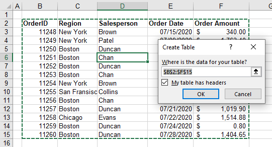
4. In the Create Table dialog box, set your cell range.

5. Mark if your table has headers.

6. Select OK.

1. Insert a table in your spreadsheet. See Overview of Excel tables for more information.

2. Select a cell within your data.

3. Select Home > Format as Table.

4. Choose a style for your table.

5. In the Create Table dialog box, set your cell range.

6. Mark if your table has headers.

7. Select OK.

To add a blank table, select the cells you want included in the table and click Insert > Table.

To format existing data as a table by using the default table style, do this:

1. Select the cells containing the data.

2. Click Home > Table > Format as Table.

3. If you don’t check the My table has headers box, Excel for the web adds headers with default names like Column1 and Column2 above the data. To rename a default header, double-click it and type a new name.

Note: You can’t change the default table formatting in Excel for the web.

Try it!

You can create and format a table, to visually group and analyze data.

1. Select a cell within your data.

2. Select Home > Format as Table.

3. Choose a style for your table.

4. In the Format as Table dialog box, set your cell range.

5. Mark if your table has headers.

6. Select OK.

Want more?

Create or delete an Excel table

Updated: 01/24/2018 by

Adding a table to your Excel spreadsheet is a quick and easy way to organize and sort data. Below are the steps on how to insert a table in Microsoft Excel.

Adding a table

1. Open Excel and move to the cell where you want to insert the table.
2. Click the Insert tab.
3. Click the Table button.

Resizing the table

Once the table is inserted, you can adjust the table’s size by moving the mouse to the bottom right corner of the table until you get a double-headed arrow. Once this arrow is visible, click-and-drag the table in the direction you want the table to expand. You can drag the cursor to the right to add more columns or down to add more rows.

Changing the look of the table

After the table is added, move your cursor to a cell in the table and click the Design tab. In the Design tab, you can adjust the Header Row, Total Row, and how the rows appear. You can also adjust the overall look of the table by clicking one of the table styles.

Using your table

Once you get the table looking the way you want it to appear, you can enter data to the table. After data is in the table, you can use the sorting features in the table by clicking the down arrow in the column you want to sort. For example, you could sort a price column from smallest to largest to identify what is the cheapest item in a list of items.

Moving the table

After adding a table, it can be moved anywhere by clicking any cell to make the table active and then hover an edge of table. When you see four arrows pointing in all directions, click and hold down the left mouse button and drag the table to the location of your choosing.

This tutorial demonstrates how to create a table in Excel.

Create an Excel Table

You can either create an Excel table using existing data, or you can create a blank table and fill it with data afterwards.

1. To create a table using existing data, ensure that your data is laid out in a way that is compatible with creating a table, e.g., each column should have a header row that describes the contents of that column and no blank rows or columns should exist in the middle or the data.

1. Then, in the Ribbon, go to Insert > Table.

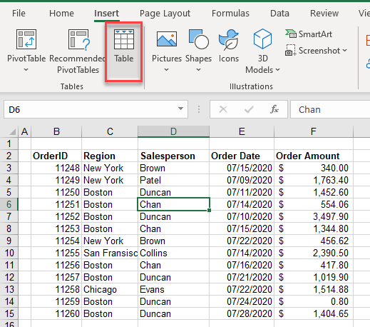
1. Excel selects the entire range of data. Leave My table has headers ticked, and then click OK.

1. This automatically creates a table as far down as the next blank row and as far across as the next blank column.

Alternate Shading in a Table

When a table is automatically created, the table is formatted according to the default table style that exists in Excel. This means that the top row is formatted with a blue background and white writing, while the rows below are formatted alternatively with a blue or white background.

1. To change the table’s appearance, click somewhere within the table and in the Ribbon, go to Table Design > Table Styles. Choose a style.

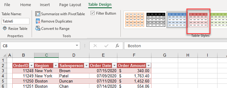
1. The format changes according to the style you choose. There are many built-in styles available. To access a few more styles, click the “more” button as shown below.

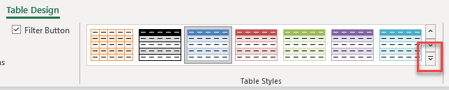
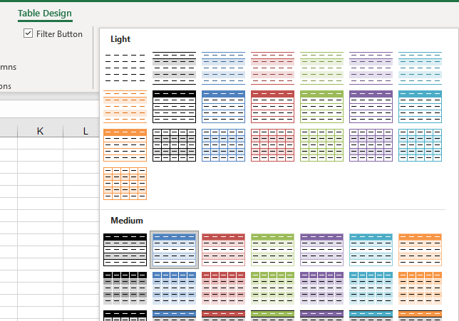
1. The list of styles is expanded to show a variety of different table styles. Choose one.

Convert Table Back to a Range

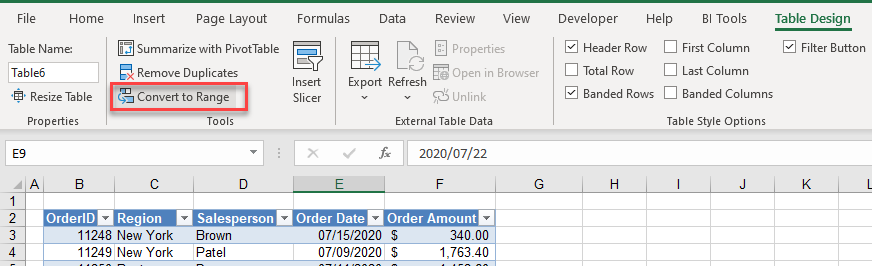
If you have formatted your data as a table, and then wish to remove the filter options and convert your table back to a range, you can use the Table Design tab to do this.

1. Click in your table, and then in the Ribbon, go to Table Design > Tools > Convert to Range.

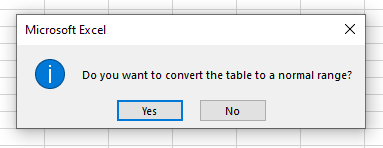
1. Click OK to convert your table to a range.

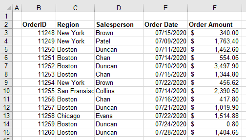
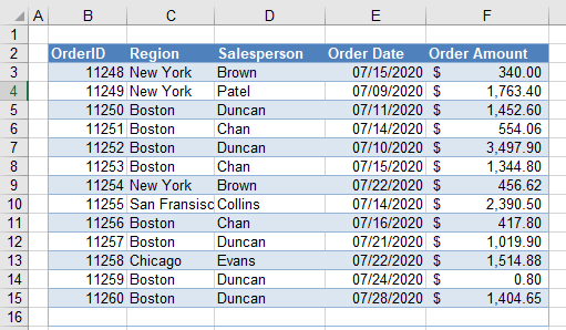
While the formatting is preserved, the filters are removed from the column headers indicating that the data is now a normal range and no longer a table.

Link Tables: Relationships

If you have data in two different ranges in Excel, but the data is linked together by a common column name, you can create a relationship between these two sets of data as long as both sets of data are tables in Excel.
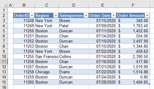
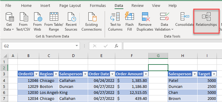
Consider the following two tables in Excel.

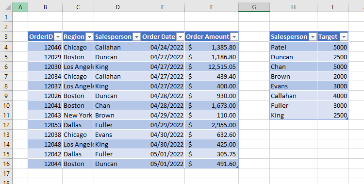
One table contains the salesperson‘s name and their Sales Target, while the other table contains their order amounts. In one table, the salesperson appears only once while in the other table the salesperson can appear multiple times.

Note: the data does not have to be on one sheet and may be much larger than the example above.

For example, to create a pivot table that contains information from both tables, you can link these tables together by creating a relationship between them.
Note: Try using some shortcuts when you’re working with pivot tables.

1. In the Ribbon, go to Data > Data Tools > Relationships.

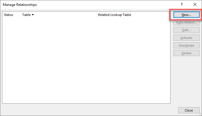
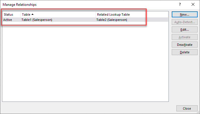
1. In the Relationships window, click New.

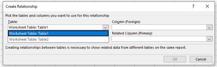
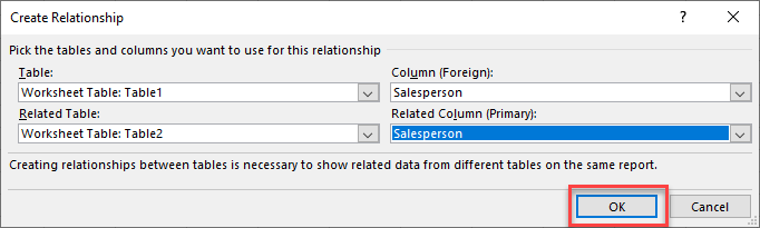
1. In the Table drop down, choose the first table and in the drop down below, choose the second table.

1. In the Column table, first choose the Foreign column (in this case, Salesperson as it can appear multiple times); and then in the Related Column, choose the Salesperson field from the second table. This is the Primary column where the salesperson only appears once in that table.

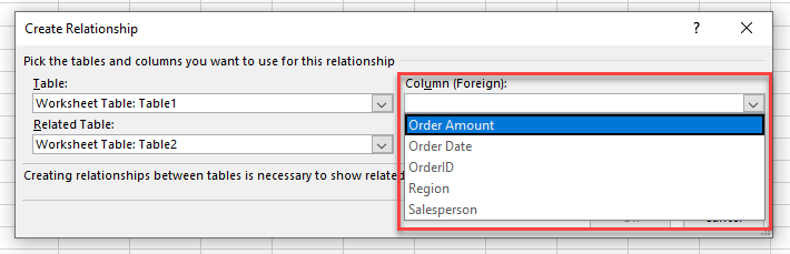
1. Click OK to create the relationship.

1. Click Close to return to Excel.

Benefits of Using a Table

Add Totals Automatically

Adding a total row to a table is incredibly easy.

Click in your table, and then, in the Ribbon, go to Table Design > Table Style Options > Total Row

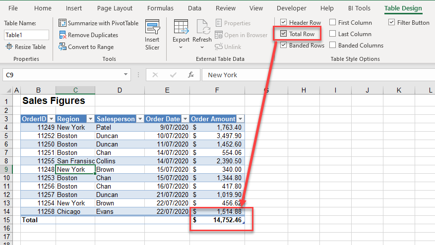
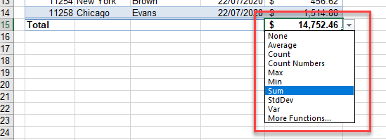
The default function use for the Total Row is the sum function. You can, however, amend this function if you want to use a different function.

Notice that the Header Row, Banded Rows, and Filter Button are also ticked in this group of options.

• If you switch off the Header Row, then the Filter Button option is no longer available.
• If you switch off the filter option, you can’t use the filter option in your table.
• you switch off the Banded Rows option, the rows are no longer alternatively shaded.

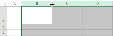
Automatically Add Rows With Tab Key

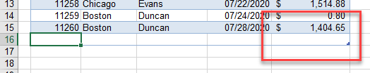
One of the benefits of using at table is that a table will automatically expand if you enter more data into the table. Notice that in the bottom row of the table, a small, backward-L-shaped handle exists.

If you then click in this cell and press the TAB key, a new row in the table is created, and your cursor is moved to the first cell in the new row. The table has therefore automatically expanded to include this row.

This is useful since some of the benefits of using a table are the sorting and filtering options that are built into the table. If you then wanted to filter on the Salesperson, for example, the new record is automatically included in that filter. Similarly, if you sort the data, the new row(s) are included in the sort.

Consistent Formulas

If you add two more columns to the table, these would automatically be included in the table, as the new rows were above.

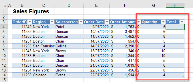
Then, add a formula to work out the total by multiplying the Order Amount by the Quantity. The formula is created using the field names (column headers).

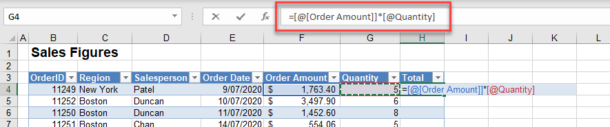
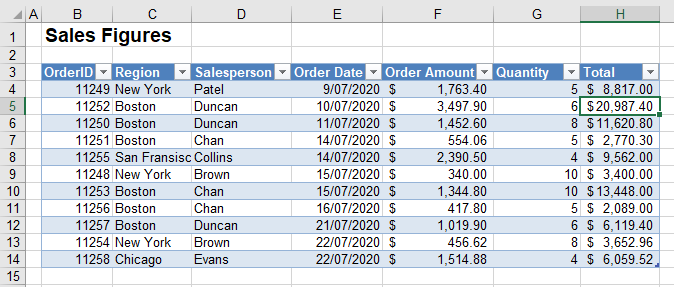
When you press ENTER, the formula is copied down to all the other rows in the table.

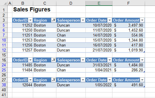
Multiple Filters on One Sheet

In the example below, a table has been created for each year of orders, and then, each table has been filtered by region to show the orders for a single region in each individual year.

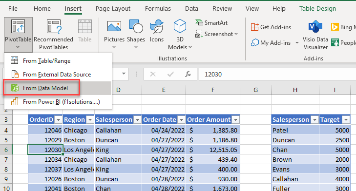
Combine Tables Into One Pivot Table

If you have created a relationship between two tables, you can create a pivot table using fields from both tables.

1. In the Ribbon, go to Insert > Pivot Table > From Data Model.

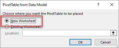
1. Select New Worksheet, and then click OK.

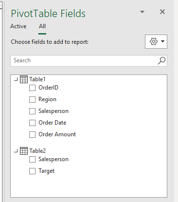
1. You now have the field available from both your tables to use in your pivot table where the linked fields (Salesperson) will show up identical data.

Able to Use Slicers

When you data is formatted as a table, you are able to use slicers to filter your data.

1. Click in your table and then, in the Ribbon, select Table Design > Tools > Insert Slicer.

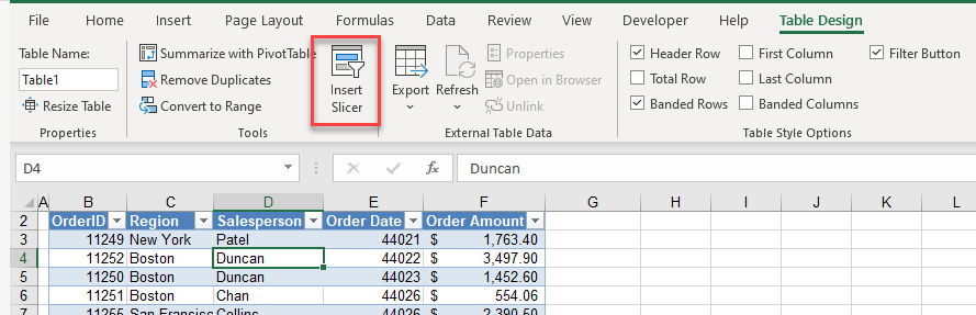
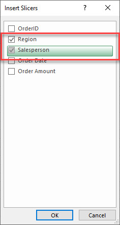
1. Select the field or fields of the slicer you wish to insert, and then click OK.

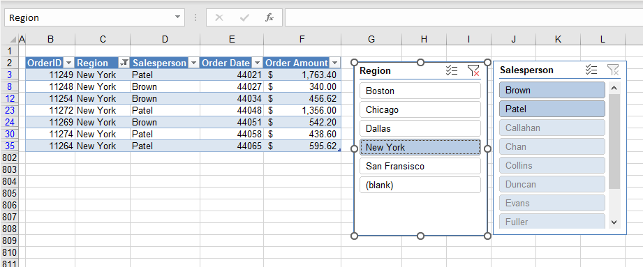
1. You can then filter your data by selecting an individual value in the slicer, or you can hold down the CTRL key (for nonconsecutive values) or the SHIFT key (for consecutive values) to filter on multiple values.

PowerPivot and Power Query

Any data used in a Power Pivot or Power Query must be in a table format. So for users of Power Query, formatting as an Excel table is a necessity, not just a benefit.

More on Tables

Tables
Add a Column and Extend a Table
Add a Total or Subtotal Row to a Table
Compare Two Tables
Convert a Table to a Normal Range
Display Data With Banded Rows
Remove a Table or Table Formatting
Rename a Table
Rotate Data Tables
Conditional Formatting	yes
Highlight Every Other Line In Excel
Copy & Paste	yes
Copy Every Other Row
Database	yes
Create a Searchable Database
Filters	yes
Filter Rows
Find & Select	yes
Select Every Other Row
Format Cells	yes
Alternate Row Color
Insert & Delete	yes
Delete Every Other Row

Creating a table in Excel may seem unusual at first. But it becomes clear that this is the best tool for solving this problem when you have mastered the first skills to work with this.

In fact Excel is a table consisting of a plurality of cells. All that is required from the user is to pick up table format for the subsequent work.



Let’s begin from next: highlight Excel cells you need using a mouse (holding the left button). After that you may choose formatting and apply it to the selected cells.

Following provisions will help to make a table in Excel as desired.

How to change the height and width of the selected cells? If you want to change cell sizes use fields with headers [A B C D] in horizontally way and [1 2 3 4] in vertically dimension. You have to move the cursor of a mouse on the border between the two cells. Holding down the left mouse button draw the border of the way and let it go.

In order not to waste time and may set the desired size to multiple cells or columns in Excel. To do this you have to activate the columns / rows by selecting them with the mouse on the gray field. It remains only to conduct already above described operation.

The window «Format Cells» can be caused by three simple ways:

1. The key combination Ctrl + 1 (the “1” is not on the numeric keypad, it’s above the letter «Q») is the fastest and most convenient way.
2. The context menu (right click).
3. Using the main menu «HOME» on the tab «Alignment».

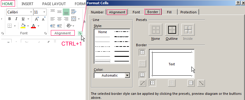
Next, perform the following steps:

1. Click on the tab «Format Cells» hovering the mouse cursor
2. A window pops up with such tabs as «Number», «Alignment», «Font», «Border», «Fill» and «Protection».
3. You must use a tabs «Border» and «Alignment» to solve this task.

Tools in «Alignment» tab are the key capabilities for effective editing previously entered text in the cells, namely:

1. Merge the selected cells.
2. The ability to transfer the words.
3. Aligning the entered text vertically and horizontally (tab located in the top menu box as well as quick access).
4. Text orientation including vertical angle.

Excel makes it possible to carry out a rapid alignment of all previously typed text in vertical orientation using the tabs located in the Main Menu.

On the «Border» tab we are working with the lines style of table borders.



Flip the table: how to do it?

For example a user has created an Excel spreadsheet file of the following form:

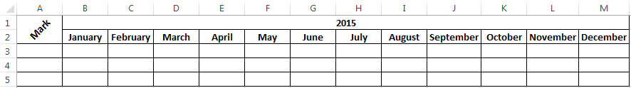
According to the task it is necessary to do so headlines in the table were positioned vertically and not horizontally as it is now. Proceed as follows.

First we need to highlight and copy the entire table. After that you must activate any empty cell in Excel. And then via the right mouse button displays a menu where you need to click the tab «Paste Special». Or you may press the key combination CTRL + ALT + V.

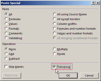
Next you need to establish a tick in the «Transpose» tab.

And press «OK» via the left button. As a result the user will receive:

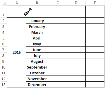
Using transposition button you can easily transfer the values even in cases where a single table header stands vertically and in the other header stands horizontally.

How to transfer values from the vertical into the horizontal table

Many users are often faced with the seemingly impossible task — transferring values from one table to another, despite the fact that values are arranged horizontally in one table, and the other placed in the vertical way.

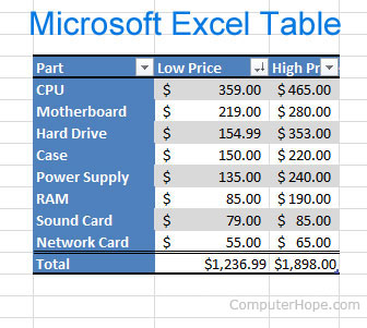
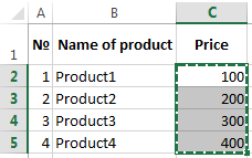
Assume that the user has an Excel price list which spelled out with the prices of the following form:

There is also a table where the total cost of the order is already calculated:

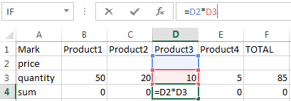
User task is to copy the values of the vertical price-list with prices and paste it into another horizontal table. It’s a long while and inconvenient to perform these actions manually by copying the value of each cell.

Use the tab «Paste Special» and transpose function in order to be able to copy all the values

Procedure:

1. The table with a price list and prices you must use the mouse to select all values. Then while holding the mouse over the previously selected field you must right-click and bring up a menu to select the «Copy»:
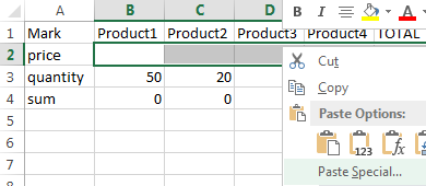
2. Then selected range will be highlighted and you may paste previously allocated prices.
3. Using the right mouse button call menu and then, you must select the button «Paste Special» while holding the cursor over the selected area.
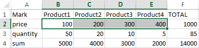
4. Finally set the check mark in «Transpose» button and press «OK».

As a result you get the following output:

Using the window «Transpose» you can completely turn the table. Function of transferring values from one table to another (taking into account their different locations) is a very handy tool. For example, it allows you to adjust the value quickly in the price list in case of the company’s pricing policy has changed.

Changing the size of the table during the adjustment in Excel

It happens often when filled Excel table simply does not fit on the screen. And you have to move from side to side which is inconvenient and time consuming. You can simply change the table scale to solve this problem. it’s very comfortably to work changing scale if you have small or big display.

To reduce the size of the table go to the tab «VIEW» and select there the tab «Zoom». Then pick up an appropriate size for your screen. For example choose 80 or 95 percent. It also might be another scale.

To increase the size of the table use the same procedure with the slight difference that the scale is placed over one hundred percent. For example choose 115 or 125 percent.

Excel offers a wide range of possibilities for building fast and efficient work. For example using a special formula (for example, = OFFSET ($a$1;0;0счеттз($а:$а);2) you can adjust the dynamic range used by the table. That can be very convenient during work especially when you are working simultaneously with multiple tables.