
One of the most common tasks in Excel is adding specific cells together. This can be as simple as adding two individual cells or more complex, like summing cells that meet certain criteria.
Fortunately, Excel offers a variety of built-in functions and tools to help you achieve this. In this article, you’ll learn how to add specific cells in Excel using eight different methods.
By understanding these techniques, you will quickly become more proficient in handling data.
Ok, let’s get into it.

How to Select Specific Cells To Add Together
Before you can add specific cells in Excel, you’ll need to select them properly. This can be done in at least four ways:
-
Using keyboard keys.
-
Using the Name Box.
-
Using named ranges.
-
Using data tables.
1. Keyboard Keys
The keys to use differ between Windows and Mac Excel. If you’re using Windows, you can click on each cell individually while holding the Ctrl key. On Mac Excel, hold the Command key down.
This is useful for selecting non-contiguous cells. The method can be tedious if you have a lot of cells, but there’s a shortcut if you’re working with a continuous range.
To select a continuous range of cells:
-
click on the first cell in the range
-
hold down the Shift key (Windows) or Command key (Mac Excel)
-
click on the last cell in the range.
2. Using the Name Box
The Name Box is located in the upper-left corner of the worksheet. You can manually type in the cell reference range (for example, A1:A5).

3. Using Named Ranges
If you find yourself frequently typing the same range, you can use named cells or ranges to make your formulas easier to read and manage. To define a named range:
-
select the cells first
-
go to the Formulas tab
-
click on Define Name

4. Using Data Tables
Data tables in Excel can help you add large amounts of data. To create a data table with the cells you want to add:
-
Select a range of cells containing your data, including headers
-
Click on the “Table” button in the “Insert” tab
-
Make sure the “My table has headers” checkbox is selected, and click “OK”
Now that you know these ways to select specific cells in Windows and Mac Excel, the following methods will let you add the values.
1. Using Excel’s Autosum Feature
The Autosum command is a built-in feature in Excel that allows you to quickly and easily calculate the sum of selected cells.
The Autosum button is located on the Home tab of the Excel ribbon, in the Editing group.

Follow these steps:
-
Select the cell where you want the sum to appear.
-
Click on the AutoSum button in the Editing group on the Home tab.
Excel will automatically try to determine the start and end of the sum range. If the range is correct, press Enter to apply the sum.
If the range is not correct, you can drag your mouse over the range of cells you wan, and then press Enter to apply the sum.
This first example shows the command summing the value of total sales:
You can also use the Autosum command across a row as well as a column. Highlight the cells in the row, choose where you want to calculate the result, and press the button.
2. Using the Excel SUM Function
You can easily add specific cells in Excel by using the SUM function. This operates on all the cells you specify.
Here is how to add specific cells in Excel using SUM():
-
Type =SUM( in a cell, followed by an opening parenthesis (.
-
Select the first cell or range to be added, for example: A1 or A1:A5.
-
If you want to add more cells or ranges, type a comma, to separate one argument from the next.
-
Select the next cell or range, such as B1 or B1:B5.
-
Continue adding cells or ranges separated by commas until all cells have been included in the formula.
-
Close the parenthesis with ) and press Enter to complete the formula and get the sum.
The result will sum values in all the cells specified. This picture shows the sum of cells A1 to A5:

Remember that the cells you’re including in the formula don’t have to be adjacent. You can add any cells in any order.
For example, if you want to add cells A2, B4, and C6, this is the SUM formula:
=SUM(A2, B4, C6)3. Addition By Cell Reference
You can also sum cells based on their cell references. This method is particularly useful when you want to add only a few particular cells in Excel that fit specific criteria.
To do this, follow the steps below:
-
Choose one cell to display the result and type an equals sign (=).
-
Select the first cell you’d like to add by clicking on it or typing its reference (e.g., A2).
-
Enter the addition operator or plus sign (+).
-
Select the second cell you’d like to add by clicking on it or typing its reference (e.g., B2).
-
Press Enter to get the result.
For example, if you want to add two cells A2 and B2, your formula would look like this:
=A2+B2If you need to add more cells, simply continue adding plus signs followed by the cell references (e.g., =A2+B2+C2). This picture shows the addition of four cells:

If you’re dealing with a larger range of cells in Excel, consider using the SUM() function I showed in the previous section.
4. Conditional Summing Using The SUMIF Function
The SUMIF function in Excel allows you to calculate sums based on a single condition. This function is useful when you want to add cells within a referenced range that meet a specific criterion.
For example, suppose you want to sum cells that contain a value greater than 5. The following formula shows the syntax:
=SUMIF(A2:A5,">5")The SUMIF function is summing all the cells in the range A2:A5 with a value greater than 5.
Here’s the step-by-step guide:
-
Select the cell where you want to display the result.
-
Type the formula containing the SUMIF function and specify the range and criteria.
-
Press Enter to complete the process.

5. Conditional Summing With The SUMIFS Function
While the SUMIF function allows you to work with a single condition, the SUMIFS function enables you to work with multiple criteria. This function is useful when you want to sum cells that meet two or more conditions.
For example, suppose you want to sum cells in column B where the corresponding cells in column A contain the text “hoodie” and column B has numbers greater than 10.
The following formula shows the syntax with filtering on text values:
=SUMIFS(B2:B7, A2:A7, "*hoodie*", B2:B7, ">10")This example formula sums the values in the range B2:B7 where the cell immediately beside them contains “hoodie” and the cells in range B2:B7 are greater than 10.
I used wildcard characters (*) to provide text filtering.

Here is how to add specific cells in Excel using multiple criteria:
-
Select the cell where you want your result to be displayed.
-
Type the SUMIFS formula mentioned above, adjusting the cell ranges and criteria as necessary.
-
Press Enter to complete the process.
Remember, both the SUMIF function and the SUMIFS function are not case-sensitive.
You can achieve even more powerful filtering if you incorporate Power Query. This video shows some of that power:
6. Using Array Formulas
An array formula is a powerful tool in Microsoft Excel for working with a variable number of cells and data points simultaneously.
First, let’s understand what an array formula is. An array formula allows you to perform complex calculations on several values or ranges at once, which means less manual work for you.
To create an array formula, you need to enter the formula using Ctrl + Shift + Enter (CSE) instead of just pressing Enter. This will surround the formula with curly braces {} and indicate that it’s an array formula.
Here is how to add specific cells in Excel using array formulas and the SUM function:
-
Select a single cell where you want the result to be displayed.
-
Type the formula =SUM(B1:B5*C1:C5) in the selected cell. This formula multiplies each value in range A1:A5 by its corresponding value in range C1:C5 and adds up the results.
-
Press Ctrl + Shift + Enter to turn this formula into an array formula.
You should now see the result of the addition in your selected cell. Remember that any changes you make to the specified cell ranges will automatically update the result displayed.

7. Using Named Ranges And The SUM Function
I showed you how to create a named range in an earlier section. Let’s now look at how to add specific cells in Microsoft Excel using a named range.
All you have to do is use the SUM function along with the named range you just created.
Let’s say we create a named range called “Prices” on cells C2 to C5 of our clothes data. To add the cells in the named range, enclose it within the SUM function as in the following formula:
=SUM(Prices)You can also use the SUMIF function with a named range.

8. Using Data Tables And The SUBTOTAL Function
When you have a data table, you can use the SUBTOTAL function to add specific cells based on certain criteria.
For this example, I created an Excel table from the clothes data I’ve used in previous sections. The table is named “Table1” and the first row is the header. The first column shows the items and the second column has the number of sales.
The following formula adds all the values in the sales column:
=SUBTOTAL(9, Table1[Sales])The syntax uses the SUBTOTAL function with two arguments:
-
The first argument is the function number for SUM, which is 9. This tells Excel to sum the values in the Sales column of Table1 that meet the specified criteria.
-
The second argument is the range of cells to be included in the calculation, which is Table1[Sales].
Another advantage of the SUBTOTAL function is that it only includes visible cells in the specified range. In contrast, the SUM function includes both hidden and visible cells.

Combining Sums With Text Descriptions
Sometimes you’ll want to have some extra text describing the result of your summed values.
For example, when you’re using conditional summing it’s a good idea to provide some context to the numbers. To do so, you can concatenate text to the result of the calculation.
Here’s an example using the SUMIF function that is summing numbers that are higher than 5. The syntax uses the & symbol to concatenate the descriptive text.
=SUMIF(B2:B25,">5") & " (total of values over five)"The example adds the characters after the sum. You can also add characters at the beginning of the cell.

Bonus Content: Adding Numbers In VBA
This article has focused on Excel formulas and functions. To round out your knowledge, I’ll quickly cover Excel VBA and macros.
In VBA, you add two or more numbers using the plus operator “+”. Here is some sample code:
Dim a as Integer,b as Integer, c as Integer
a = 3
b = 2
c = a + b
MsgBox "The sum of " & a & " and " & b & " is " & c
In this example, we declared three variables: a, b, and c, all of which are of type Integer. We assigned the values 2 and 3 to a and b.
Then we added a and b together using the “+” operator and assigned the result to the variable c. The last line displays the values of a and b along with the calculated sum of c.
5 Common Errors to Avoid
When working with Microsoft Excel formulas, it’s essential to avoid common errors that might lead to inaccurate results or disrupt your workflow. Here are five errors to steer clear of.
1. Incorrect Formatting
You may see a #NUM! error or a result of zero if the cells you’re working with are not formatted correctly. The problem can be with a single cell.
When cells have text values, some functions simply skip those cells. Others will show a Microsoft error code. Be sure to format your target cells as numbers.
The problem can occur when you have copied numeric data that has unsupported formatting. For example, you may have copied a monetary amount formatted like “$1,000”. Excel may treat this as a text value.
To avoid issues, enter the values as numbers without formatting. When you are copying data, you can use Paste Special to strip the formatting from the destination cell.
2. Unnecessary Merging of Cells
Try to avoid merging and centering cells across a row or column. This may interfere with selecting cell ranges and cause issues when working with formulas like the SUMIF function.
Instead, consider using the “Center Across Selection” option for formatting purposes. Follow these steps:
-
Select the cells
that you want to apply the formatting to
-
Right-click on the selected cells and choose “Format Cells” from the context menu
-
In the “Format Cells” dialog box, click on the “Alignment” tab
-
Under “Horizontal”, select “Center Across Selection” from the dropdown menu

3. Incorrect Argument Separators
Depending on your location settings, you might be required to use a comma or a semi-colon to separate arguments in a formula.
For example, =SUM(A1:A10, C1:C10) might need to be =SUM(A1:A10; C1:C10) in certain regions.
Not using the correct separator can cause errors in your calculations.
4. Handling of Errors in Cell Values
When summing specific cells, it’s common for some to contain errors, such as #N/A or #DIV/0. These errors can disrupt your overall results if not handled properly.
A helpful solution is to use the IFERROR function or the AGGREGATE function to ignore or manage error values.
For instance, you can sum a range while ignoring errors by applying the formula =AGGREGATE(9,6,data), where ‘data’ is the named range with possible errors.
5. Using Criteria Without Quotation Marks
When summing cells based on criteria such as greater than or equal to specific values, be sure to enclose the criteria expression in quotation marks.
For example, when using SUMIF, the correct formula is =SUMIF(range, “>500”, sum_range), with quotation marks around the >500 criteria.
By keeping these common errors in mind and applying the suggested solutions, you can improve your Microsoft Excel skills and ensure your calculations are accurate and efficient.
Our Final Say – It’s Time For You To Excel!
You now know how to add specific cells in Excel using eight different methods and formulas. The many examples show how to sum numbers based on a selected range.
You also know how each formula works and when to use them. Each Excel formula is available in recent editions of Excel, including Excel for Microsoft 365.
Some produce the same result, while others allow different ways to filter the data on selected cells.
Best of luck on your data skills journey.
On another note, if you are looking to master the Microsft stack and take your data skills to the next level, check out our free training.
How to Add Cells in Excel (Table of Contents)
- Adding Cells in Excel
- Examples of Add Cells in Excel
Adding Cells in Excel
Adding a cell is nothing but inserting a new cell or group of cells in between the existing cells by using the insert option in excel. We can insert the cells in row-wise or column-wise as per requirement, which allows us to input the additional data or new data in between the existing data.
Explanation: Sometimes, while working with Excel, we may forget to add some portion of date that should be inserted in between the existing data. In that case, we can cut the data and paste it a bit down or right and can input the required data in the gap. However, we can achieve the same without using the cut and paste option but by using the insert option in Excel.
There are four different options available to insert new cells. We will see each option and the respective example.
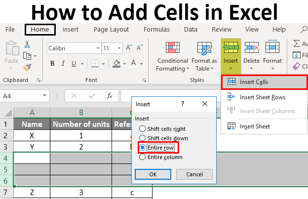
We can insert new cells in two ways; one way is to select the insert option from the worksheet, and the other is the shortcut key. Click on the “Home” menu at the top left corner in case if you are in a different menu.
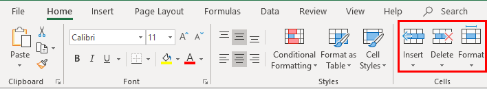
After the selection of “Home”, observe the right-hand side we have a section called “cells”. Which covers the options like “Insert”, “Delete”, and “format”, which are highlighted with a red colour box.
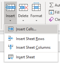
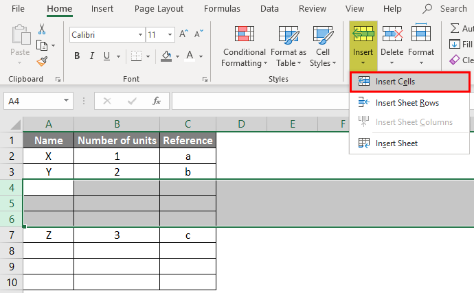
Each option has a drop-down if we observe under each option name. Click on the Insert option drop down then the drop-down menu will appear as below.
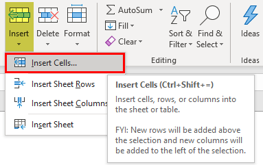
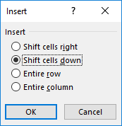
It has four different options: insert cells, insert sheet rows, insert sheet columns, and insert sheet. Click on the option Insert cells; then it will open a pop-up menu with four options as below.
Examples of Add Cells in Excel
Here are some examples of How to Add Cells in Excel, which are given below
You can download this How to Add Cells Excel Template here – How to Add Cells Excel Template
Example #1 – Add a Cell using Shift Cells Right
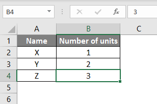
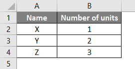
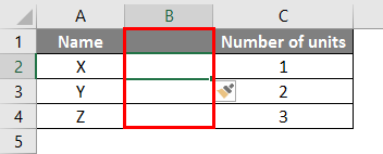
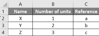
Consider a table having data of two columns like below.

Now it has three rows of data. But in case if we need to add a cell at the cell B4 by moving the data to the right, we can do that. Follow the steps.
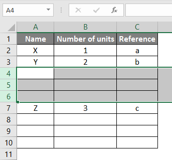
Step 1: Select the cell where you want to add a new cell. Here we have selected B4 as shown below.
Step 2: Select the Insert menu option for the drop-down as below.
Step 3: Select the Insert Cells option then a pop-up menu will appear as below.
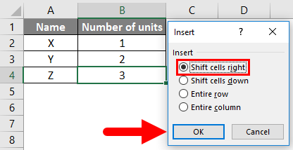
Step 4: Select the “Shift cells right” option, then click on OK. Then the result will appear as below.
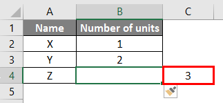
If we observe the above screen, number 3 is shifted to the right and created a new empty cell. This is how “shift cell right” will work. Similarly, we can do the shift cells down also.
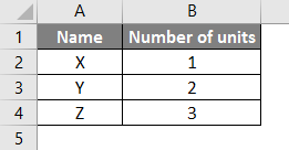
Example #2 – Insert a New Column and New Row
To add a new column, follow the below steps. It is as similar to shifting cells.
Step 1: Consider the same table which we took in the above example. Now we need to insert a column in between the two columns.
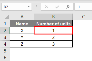
Step 2: A column will always be added on the left-hand side; hence select any one cell in the number of units as below.
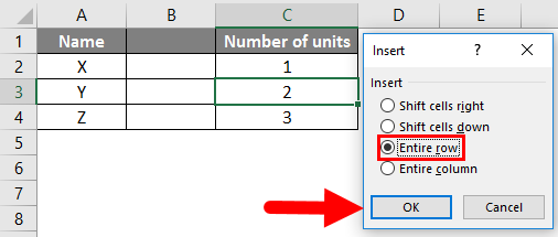
Step 3: Now select the “Entire column” option from the insert option as shown in the below image.
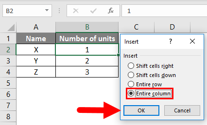
Step 4: Select the OK button. A new column will be added in between the existing two columns as below.
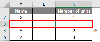
In a similar way, we can add the row by clicking the Entire row option as below.
The result will be as below. A new row is added between the data X and Y.
Example #3 – Adding Rows After Each Row using the Sort Option
Up to now, we covered how to add a single cell by shifting cells right and down, adding an entire row an entire column.
But these actions will affect only one row or one column. In case if we want to add an empty row under each existing row, we can perform in another way. Follow the below steps to add an empty row.
Step 1: Take the same table which we used in the previous example.
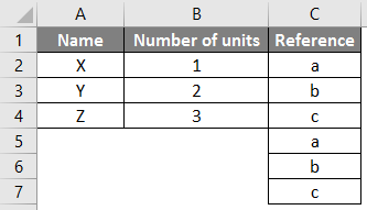
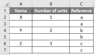
Step 2: Take some reference for the time being column ‘C’ as below.
Step 3: Now copy the references and paste them in under the last reference in the table as below.
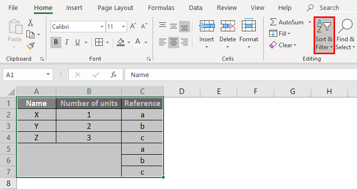
Step 4: To add an empty line under each existing data line, we are using a sorting option. Highlight the entire table and click on the sort option. It is available under “Home”, highlighted in the below picture for reference.
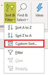
Step 5: From the drop-down of the Sort option, select the custom sort.
Step 6: A window will open as below.
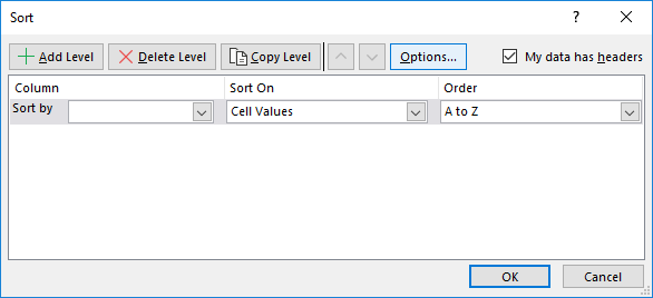
Step 7: From Sort by select the “Reference” option as shown in the below image.
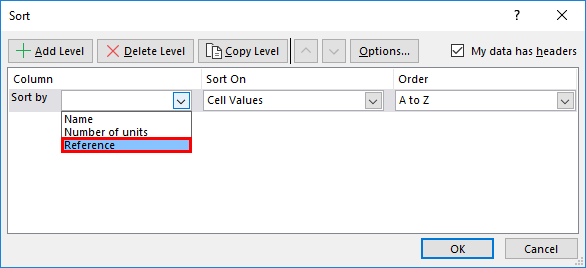
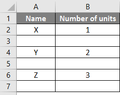
Step 8: Select OK, then see it will sort in such an empty line between each data existing line as below.
Step 9: Now, we can remove the reference column. I hope you understand why we added the reference column.
Example #4 – Adding Multiple Rows or Columns or Cells
If we want to add multiple lines or cells at the same time, highlight the number of cells or lines that you required and perform the insert option as per selection. If we select the multiple row lines as below.
Now use the insert option, which we add for rows.
The moment we select “insert cells”, it will directly add the rows without asking for another pop-up as how it asked before. Here we highlighted 3 lines; hence when we click on “Insert Cells”, it will add another 3 empty lines under the selected lines.
Things to Remember
- “Alt + I” is the shortcut key to add a cell or line in the excel spreadsheet.
- A new cell can be added only on the right-hand side and down only. We cannot add the cells to the left and up; hence whenever you want to add the cells to highlight the cell as per this rule.
- A row will always be added at the bottom of the highlighted cell.
- A column will always be added on the left side of the highlighted cell.
- If you want to add multiple cells or rows at a time, highlight multiple cells or rows.
Recommended Articles
This is a guide on How to Add Cells in Excel. Here we discuss How to Add Cells along with examples and downloadable excel template. You may also look at the following articles to learn more –
- How to Sum Multiple Rows in Excel
- SUM Cells in Excel
- Count Cells with Text in Excel
- Excel Shortcut For Merge Cells
![]()
Download Article
![]()
Download Article
Need to find the sum of a column, row, or set of numbers in Excel? Microsoft Excel comes with many mathematical functions, including multiple ways to add sets of numbers. This wikiHow article will teach you the easiest ways to add numbers, cell values, and ranges in Microsoft Excel.
-

1
Click the cell in which you want to display the sum.
-
2
Type an equal sign =. This indicates the beginning of a formula.
Advertisement
-
3
Type the first number you want to add. If you would rather add the value of an existing cell instead of typing a number manually, just click the cell you want to include in the equation. Otherwise, you can type a number manually.
- For example, if you click cell C3, the value of C3 will be the first number in your equation. If you type 1, the number 1 will be the first number in your equation.
-
4
Type a + sign.
-
5
Type another number select another cell. This adds the second number or value to your equation.
- You can add multiple cells or numbers at once if you’d like—just separate each number or address with another + sign.[1]
- For example, if you want to find the sum of cells C3, D4, and E5, your formula will look like this =C3+D4+E5.
- If you want to add 1 plus 1, your formula will look like this: =1+1 .
- You can add other operations, such as subtraction or multiplication, in the same equation. In this example, we’ll add the values of C3 and D4 and then subtract 2: =C3+D4-2
- You can add multiple cells or numbers at once if you’d like—just separate each number or address with another + sign.[1]
-
6
Press ↵ Enter or ⏎ Return. Now you’ll see the sum of the added numbers or values in the selected cell.


Advertisement
-
1
Click the cell in which you want to display the sum. The SUM function works like using the plus + sign, but is a bit easier to work with when you’re adding multiple cells and ranges.
-
2
Type an equal sign followed by the word SUM =SUM. This indicates the beginning of the SUM formula.
-
3
Type an opening parenthesis (. Your formula should now look like this: =SUM(.
-
4
Select the range of cells you want to add. Click and drag over all of the cells you want to add together. For example, if you want to add the values of all cells from A1 through A10, select all of those cells now.
- You can also select multiple columns and rows here. To select multiple non-adjacent columns and/or rows, hold down the Control key and as you select each range.
- You don’t have to select entire ranges with the SUM function—you can also enter individual numbers or cell addresses.
-
5
Type a clothing parenthesis ). This finishes the formula.
- Your formula should now look something like this: =SUM(B4,B8)
- In this example, we’ve selected cells B4 through B8
- If you selected non-adjacent ranges, each range will be separated by a comma. In this example, we selected B4 through C8 (two adjacent columns) and E4 through E5: =SUM(B4:C8,E4:E5)
- Your formula should now look something like this: =SUM(B4,B8)
-
6
Press ↵ Enter or ⏎ Return. The sum of the selected range now appears in this cell.


Advertisement
-
1
Click the cell immediately below or next to the values you want to add. AutoSum will automatically create a formula that adds the values of an adjacent column or row.[2]
- For example, if you want to add the values of cells A:2 through A:10, you would click cell A11.
- You can also add multiple columns or rows at the same time by selecting multiple cells. For example, to display the sums of values in columns A, B, and C, you could select cells A11, B11, and C11.
-
2
Click the AutoSum icon on the Home tab Σ. It’s the Sigma icon (which looks like an «E») on the Home tab at the top of Excel. A formula will then appear in the selected cell.
-
3
Press ↵ Enter or ⏎ Return. Now you’ll see the results of the formula in the cell.
- If you selected multiple blank cells, you’ll see each individual column or row’s value in the selected cells.


Advertisement
Ask a Question
200 characters left
Include your email address to get a message when this question is answered.
Submit
Advertisement
-
Use the SUMIF function to add cells that match certain criteria. For example, if you wanted to find the sum of all cells in A2 through A:10 that are greater than 1, you’d use =SUMIF(A2:A10, ">1").[3]
Thanks for submitting a tip for review!
Advertisement
About This Article
Article SummaryX
1. Use a plus sign to write out formulas like this: =4+5
2. Use the SUM formula to add values from one or more ranges.
3. Use AUTOSUM to automatically find the total of a column or row.
Did this summary help you?
Thanks to all authors for creating a page that has been read 108,680 times.
Is this article up to date?
Insert cells
- Select the cell, or the range of cells, to the right or above where you want to insert additional cells.
- Hold down CONTROL, click the selected cells, then on the pop-up menu, click Insert.
- On the Insert menu, select whether to shift the selected cells down or to the right of the newly inserted cells.
Contents
- 1 Can you insert a single cell in Excel?
- 2 How do I insert a blank cell between data in Excel?
- 3 How do I insert one cell?
- 4 How do you insert a cell in Excel using the keyboard?
- 5 How will you enter cells in a worksheet?
- 6 How do I put multiple cells into one cell?
- 7 How do you automatically insert rows in Excel?
- 8 How can u activate a cell?
- 9 How do I open a cell in Excel?
- 10 What does Ctrl Shift do in Excel?
- 11 How do you combine cells in Excel without losing data?
- 12 How do I insert text into Excel?
- 13 How do I sum all 7 cells in Excel?
- 14 How do you add all 12 cells in Excel?
- 15 How do you add all three cells in Excel?
- 16 How do you insert cells in Excel without changing formulas?
- 17 How do I add a row to a cell value in Excel?
- 18 Which of the following is an active cell in Excel?
- 19 What symbol is used before adding the function?
- 20 How can you activate a cell in MS Excel by clicking on it by pressing the arrow keys by pressing Tab key all of the above?
Can you insert a single cell in Excel?
To add a new individual cell to an Excel spreadsheet, follow the steps below. Select the cell of where you want to insert a new cell by clicking the cell once with the mouse. Right-click the cell of where you want to insert a new cell. In the right-click menu that appears, select Insert.
How do I insert a blank cell between data in Excel?
Select the cells where the empty rows need to appear and press Shift + Space. When you pick the correct number of rows, right-click within the selection and choose the Insert option from the menu list. Tip. If your cells contain any formatting, use the Insert Options icon to match the format.
How do I insert one cell?
To insert a single cell:
- Right-click the cell above which you want to insert a new cell.
- Select Insert, and then select Cells & Shift Down.
How do you insert a cell in Excel using the keyboard?
Your options are:
- Ctrl + Shift + “+” + I: Shifts cells right to insert cell.
- Ctrl + Shift + “+” + D: Shift cells down to insert cell.
- Ctrl + Shift + “+” + R: Inserts entire row.
- Ctrl + Shift + “+” + C: Inserts entire column.
How will you enter cells in a worksheet?
Enter text or a number in a cell
- On the worksheet, click a cell.
- Type the numbers or text that you want to enter, and then press ENTER or TAB. To enter data on a new line within a cell, enter a line break by pressing ALT+ENTER.
How do I put multiple cells into one cell?
Combine data with the Ampersand symbol (&)
- Select the cell where you want to put the combined data.
- Type = and select the first cell you want to combine.
- Type & and use quotation marks with a space enclosed.
- Select the next cell you want to combine and press enter. An example formula might be =A2&” “&B2.
How do you automatically insert rows in Excel?
Fortunately, there are shortcuts that can quickly insert blank row in Excel. Select the entire row which you want to insert a blank row above, and press Shift + Ctrl + + keys together, then a blank row is inserted.
How can u activate a cell?
Answer: D. A cell can be ready to activate by any of the method Pressing the Tab key or Clicking the cell or Pressing an arrow key.
How do I open a cell in Excel?
You can also press Ctrl+Shift+F or Ctrl+1. In the Format Cells popup, in the Protection tab, uncheck the Locked box and then click OK. This unlocks all the cells on the worksheet when you protect the worksheet.
What does Ctrl Shift do in Excel?
Press Ctrl + Shift + $ to apply Currency format, Ctrl + Shift + ~ to apply General number format, Ctrl + Shift % to apply Percentage format, Ctrl + Shift + # to apply Date format, Ctrl + Shift + @ to apply Time format, Ctrl + Shift + ! to apply Number format with two decimal places and thousands separator, and Ctrl +
How do you combine cells in Excel without losing data?
How to merge cells in Excel without losing data
- Select all the cells you want to combine.
- Make the column wide enough to fit the contents of all cells.
- On the Home tab, in the Editing group, click Fill > Justify.
- Click Merge and Center or Merge Cells, depending on whether you want the merged text to be centered or not.
How do I insert text into Excel?
To add certain text or character to the beginning of a cell, here’s what you need to do:
- In the cell where you want to output the result, type the equals sign (=).
- Type the desired text inside the quotation marks.
- Type an ampersand symbol (&).
- Select the cell to which the text shall be added, and press Enter.
How do I sum all 7 cells in Excel?
With the help of the SUM function, we can achieve that. The formula to calculate the sum of the first seven rows will be =SUM (OFFSET ($B$2, (ROW ()-ROW ($B$2))*7, 0, 7, 1)). In this formula, B2 represents the column with the header price, this is the column with the numeric values that we need to sum.
How do you add all 12 cells in Excel?
How to sum every n rows down in Excel?
- Enter this formula into a blank cell where you want to put the result: =SUM(OFFSET($B$2,(ROW()-ROW($B$2))*5,0,5,1))
- Tip: In the above formula, B2 indicates the started row number you want to sum, and 5 stands for the incremental row numbers.
How do you add all three cells in Excel?
How to Sum Every 3 Cells
- =SUM(OFFSET(REFERENCE, ROWS, COLUMN(S), HEIGHT, WIDTH))
- =SUM(OFFSET($B4,0,(COLUMN()-COLUMN($H$4))*3,1,3))
- =SUM(OFFSET($B4,0,(COLUMN()-COLUMN($H$4))*3,1,3))
- (COLUMN()-COLUMN($H$4))*3.
How do you insert cells in Excel without changing formulas?
Select the formula in the cell using the mouse, and press Ctrl + C to copy it. Select the destination cell, and press Ctl+V. This will paste the formula exactly, without changing the cell references, because the formula was copied as text.
How do I add a row to a cell value in Excel?
Press Alt + F11 keys simultaneously, and a Microsoft Visual Basic for Applications window pops out. 2. Click Insert > Module, then paste below VBA code to the popping Module window. VBA: Insert row below based on cell value.
Which of the following is an active cell in Excel?
Detailed Solution. The correct answer is Current cell. Alternatively referred to as a cell pointer, current cell, or selected cell, an active cell is a rectangular box that highlights the cell in a spreadsheet.
What symbol is used before adding the function?
Just like a basic formula, you need to start with the equal sign. After that, you would put the function name, then the range of cells inside parentheses, separated with a colon. For example: =SUM(B2:B5).
How can you activate a cell in MS Excel by clicking on it by pressing the arrow keys by pressing Tab key all of the above?
Therefore, arrow keys also help us in activating cell. So, all the three methods, i.e, pressing the tab key, clicking the cell and pressing an arrow key help us in activating cell.
Содержание
- Процедура добавления ячеек
- Способ 1: Контекстное меню
- Способ 2: Кнопка на ленте
- Способ 3: Горячие клавиши
- Вопросы и ответы

Как правило, для подавляющего большинства пользователей добавление ячеек при работе в программе Excel не представляет сверхсложной задачи. Но, к сожалению, далеко не каждый знает все возможные способы, как это сделать. А ведь в некоторых ситуациях применение именно конкретного способа помогло бы сократить временные затраты на выполнение процедуры. Давайте выясним, какие существуют варианты добавления новых ячеек в Экселе.
Читайте также: Как добавить новую строку в таблице Эксель
Как вставить столбец в Excel
Процедура добавления ячеек
Сразу обратим внимание на то, как именно с технологической стороны выполняется процедура добавления ячеек. По большому счету то, что мы называем «добавлением», по сути, является перемещением. То есть, ячейки просто сдвигаются вниз и вправо. Значения, которые находятся на самом краю листа, таким образом, при добавлении новых ячеек удаляются. Поэтому нужно за указанным процессом следить, когда лист заполняется данными более, чем на 50%. Хотя, учитывая, что в современных версиях Excel имеет на листе 1 миллион строк и столбцов, на практике такая необходимость наступает крайне редко.
Кроме того, если вы добавляете именно ячейки, а не целые строки и столбцы, то нужно учесть, что в таблице, где вы выполняете указанную операцию, произойдет смещение данных, и значения не будут соответствовать тем строкам или столбцам, которым соответствовали ранее.
Итак, теперь перейдем к конкретным способам добавления элементов на лист.
Способ 1: Контекстное меню
Одним из самых распространенных способов добавления ячеек в Экселе является использование контекстного меню.
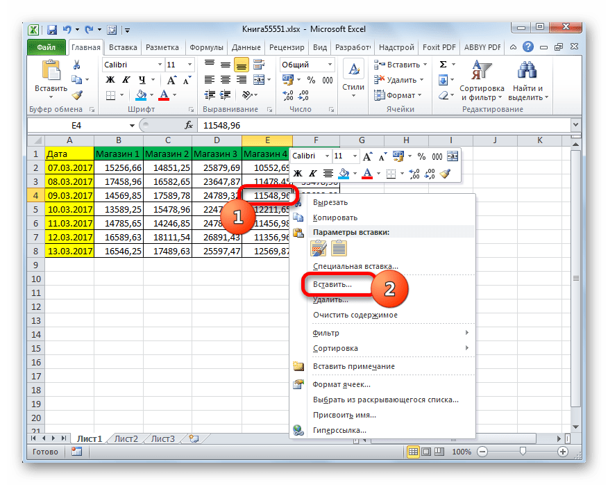
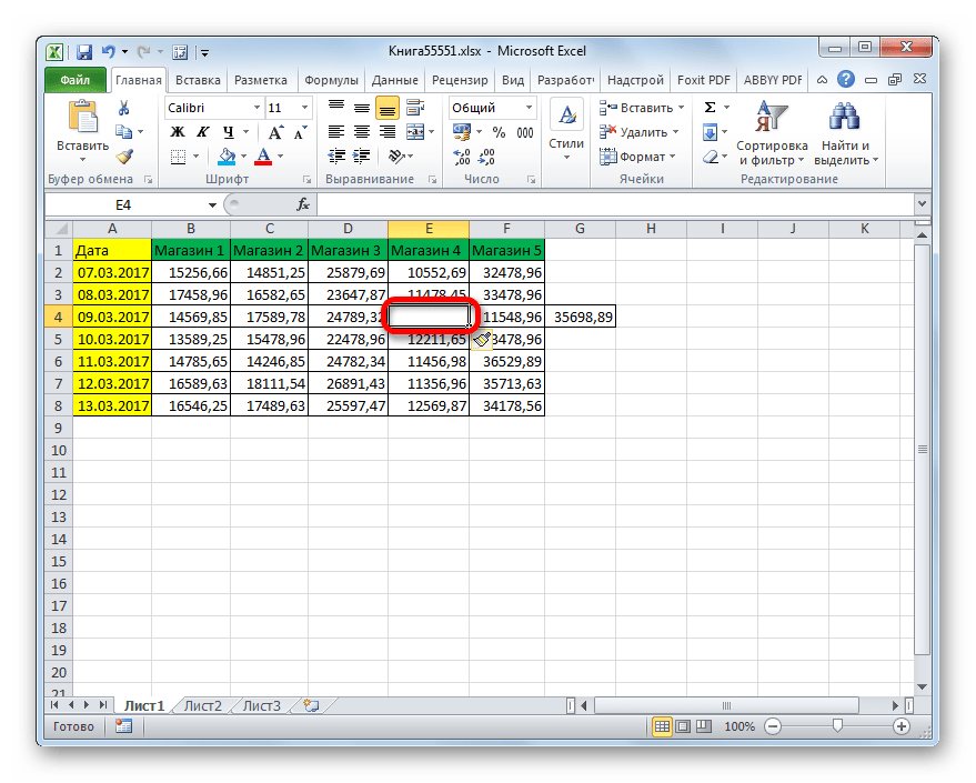
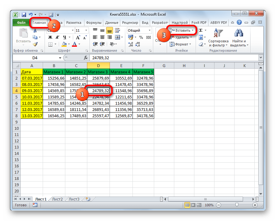
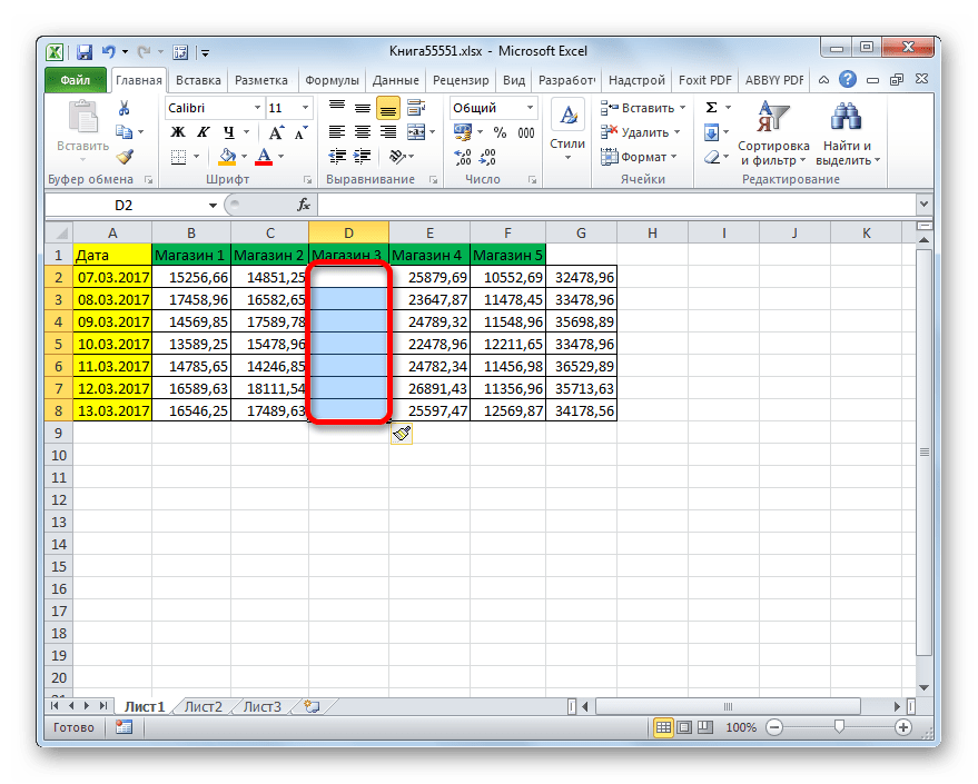
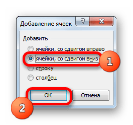
- Выделяем элемент листа, куда хотим вставить новую ячейку. Кликаем по нему правой кнопкой мыши. Запускается контекстное меню. Выбираем в нем позицию «Вставить…».
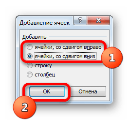
- После этого открывается небольшое окошко вставки. Так как нас интересует именно вставка ячеек, а не целых строк или столбцов, то пункты «Строку» и «Столбец» мы игнорируем. Производим выбор между пунктами «Ячейки, со сдвигом вправо» и «Ячейки, со сдвигом вниз», в соответствии со своими планами по организации таблицы. После того, как выбор произведен, жмем на кнопку «OK».
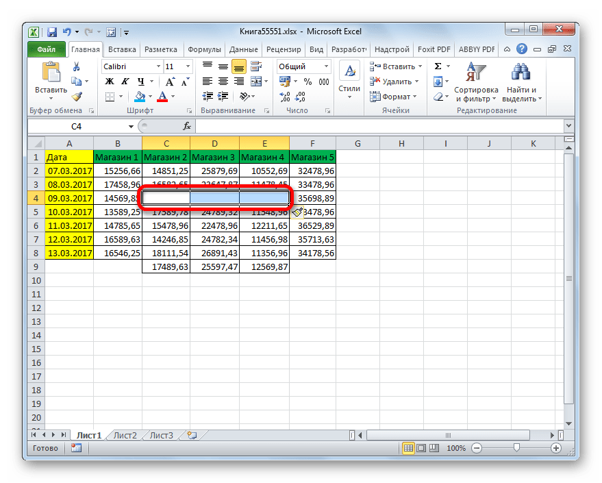
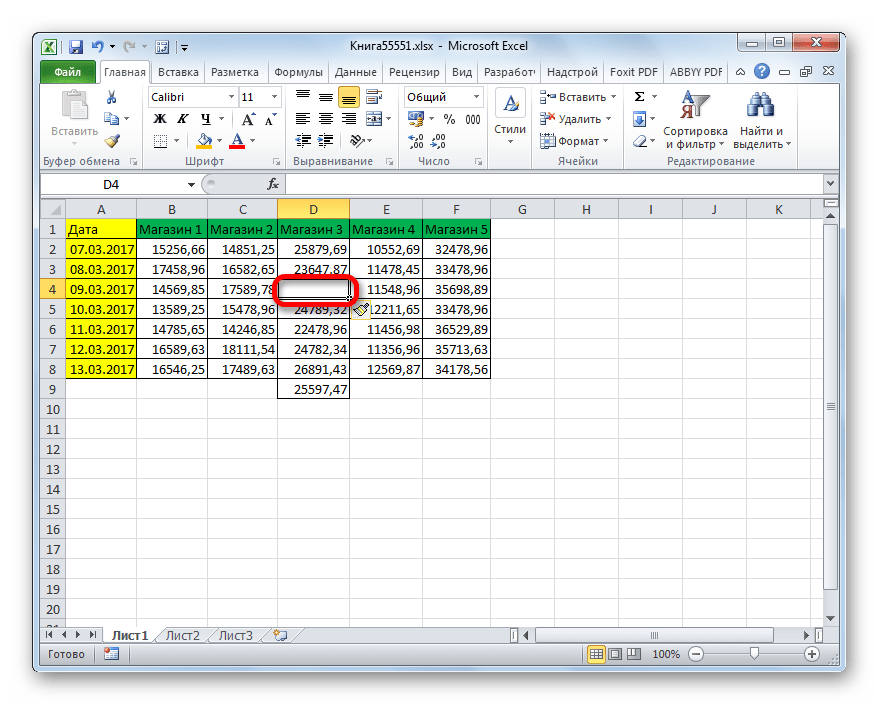
- Если пользователь выбрал вариант «Ячейки, со сдвигом вправо», то изменения примут примерно такой вид, как на таблице ниже.

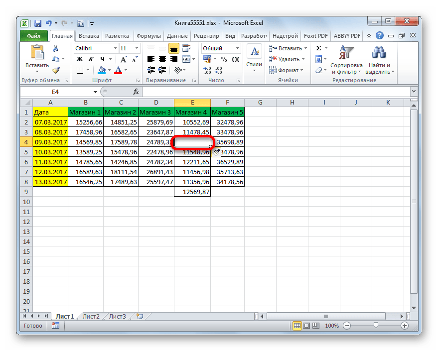
Если был выбран вариант и «Ячейки, со сдвигом вниз», то таблица изменится следующим образом.
Аналогичным образом можно добавлять целые группы ячеек, только для этого перед переходом в контекстное меню нужно будет выделить соответствующее число элементов на листе.
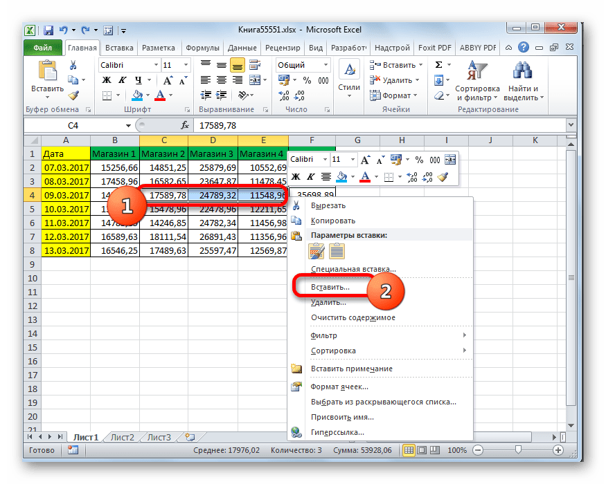
После этого элементы будут добавлены по тому же алгоритму, который мы описывали выше, но только целой группой.

Способ 2: Кнопка на ленте
Добавить элементы на лист Excel можно также через кнопку на ленте. Посмотрим, как это сделать.
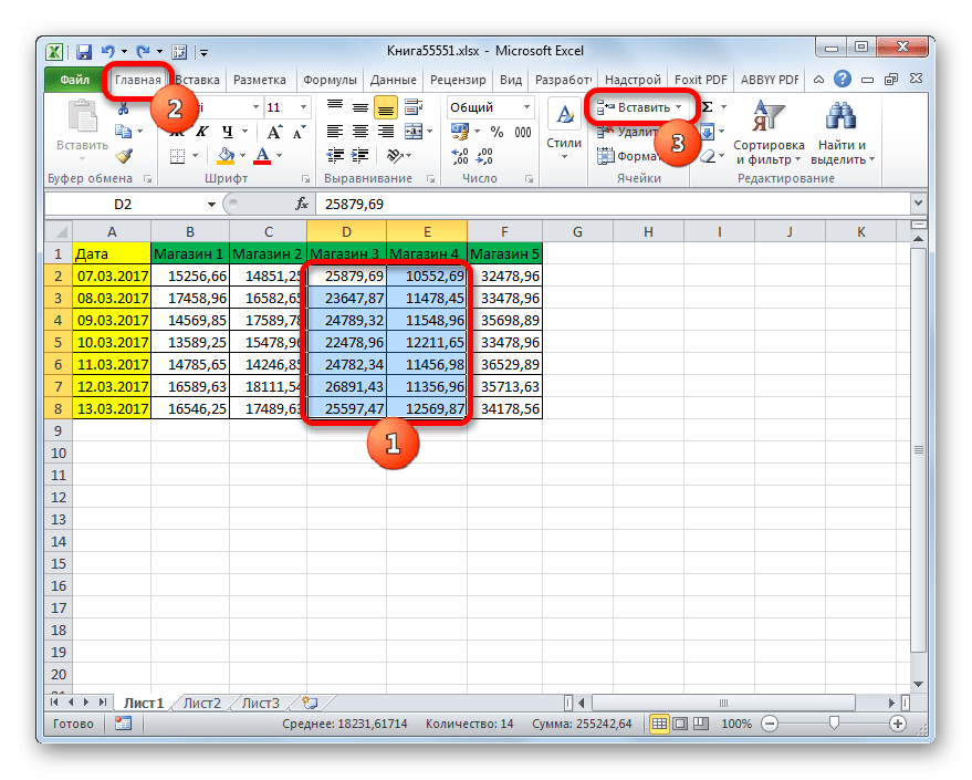
- Выделяем элемент на том месте листа, где планируем произвести добавление ячейки. Перемещаемся во вкладку «Главная», если находимся в данный момент в другой. Затем кликаем по кнопке «Вставить» в блоке инструментов «Ячейки» на ленте.
- После этого элемент будет добавлен на лист. Причем, в любом случае он будет добавлен со смещением вниз. Так что данный способ все-таки менее гибок, чем предыдущий.
С помощью этого же способа можно производить добавление групп ячеек.
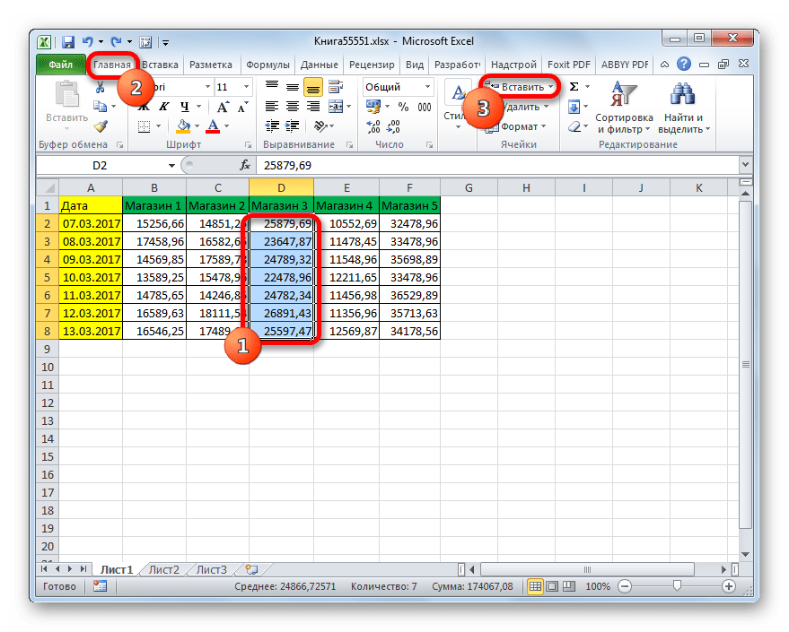
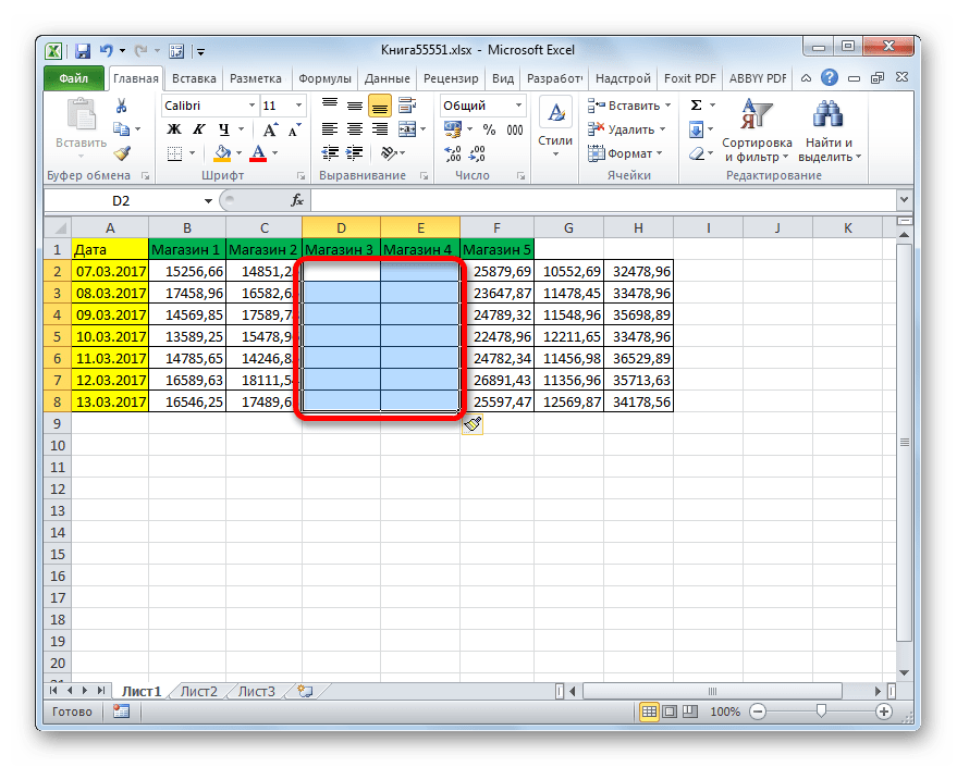
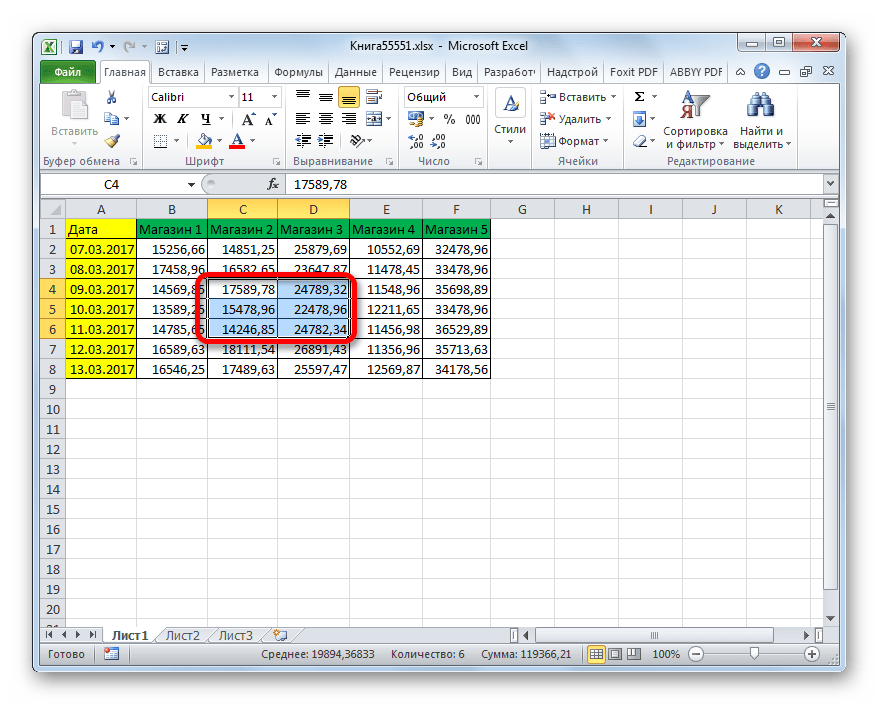
- Выделяем горизонтальную группу элементов листа и жмем на знакомую нам иконку «Вставить» во вкладке «Главная».
- После этого группа элементов листа будет вставлена, как и при одиночном добавлении, со сдвигом вниз.
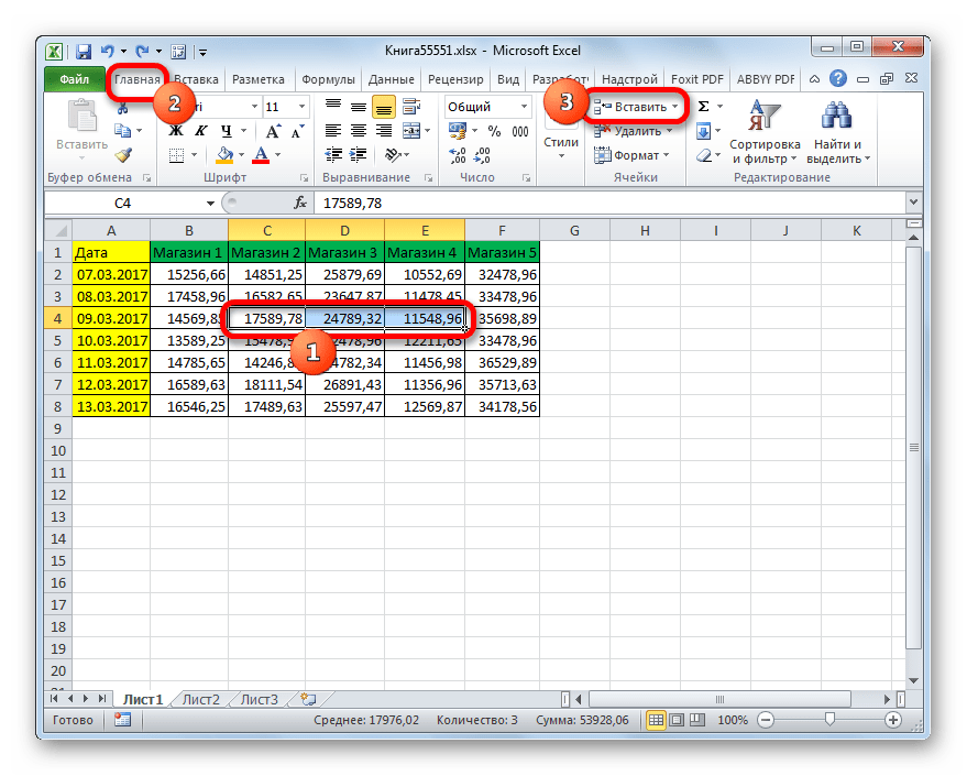

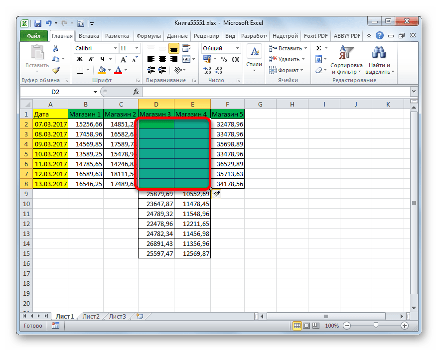
А вот при выделении вертикальной группы ячеек мы получим несколько иной результат.
- Выделяем вертикальную группу элементов и жмем на кнопку «Вставить».
- Как видим, в отличие от предыдущих вариантов, в этом случае была добавлена группа элементов со сдвигом вправо.
Что же будет, если мы этим же способом добавим массив элементов, имеющий как горизонтальную, так и вертикальную направленность?
- Выделяем массив соответствующей направленности и жмем на уже знакомую нам кнопку «Вставить».
- Как видим, при этом в выделенную область будут вставлены элементы со сдвигом вправо.
Если же вы все-таки хотите конкретно указать, куда должны сдвигаться элементы, и, например, при добавлении массива желаете, чтобы сдвиг произошел вниз, то следует придерживаться следующей инструкции.
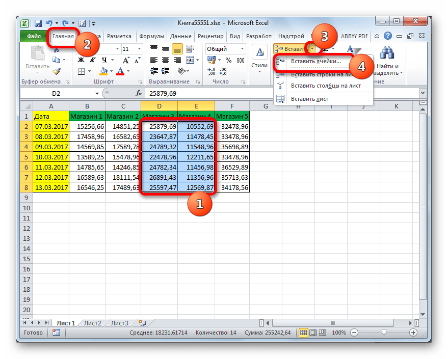
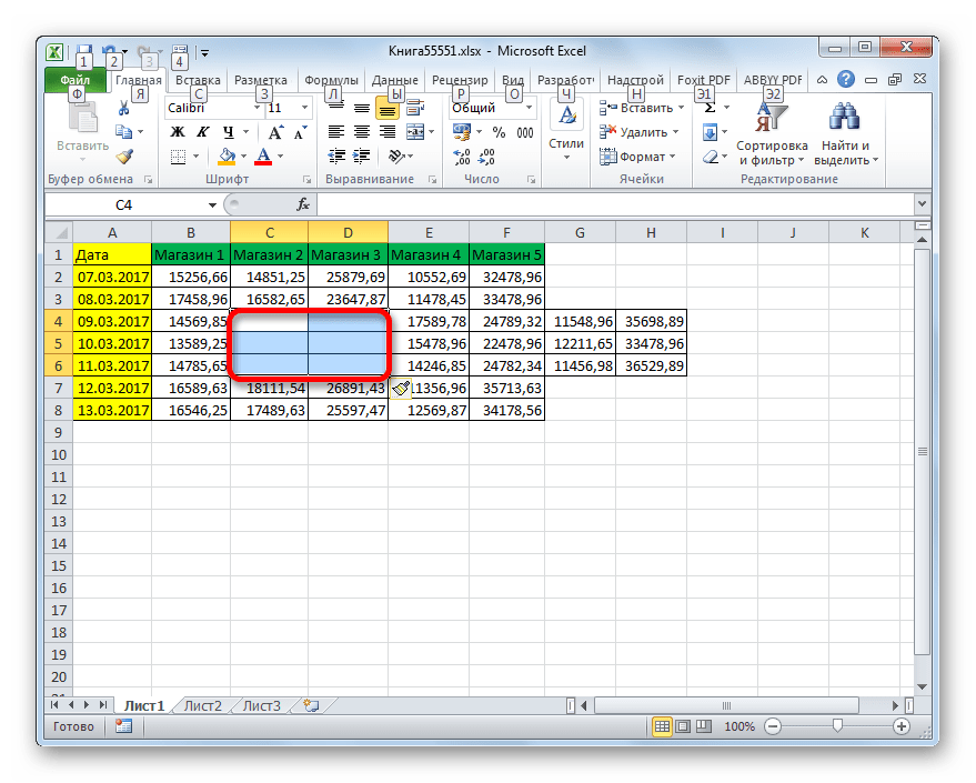
- Выделяем элемент или группу элементов, на место которой хотим произвести вставку. Щелкаем не по знакомой нам кнопке «Вставить», а по треугольнику, который изображен справа от неё. Открывается список действий. Выбираем в нем пункт «Вставить ячейки…».
- После этого открывается уже знакомое нам по первому способу окошко вставки. Выбираем вариант вставки. Если мы, как было сказано выше, хотим произвести действие со сдвигом вниз, то ставим переключатель в позицию «Ячейки, со сдвигом вниз». После этого жмем на кнопку «OK».
- Как видим, элементы были добавлены на лист со сдвигом вниз, то есть, именно так, как мы задали в настройках.
Способ 3: Горячие клавиши
Самый быстрый способ добавить элементы листа в Экселе – это воспользоваться сочетанием горячих клавиш.
- Выделяем элементы, на место которых хотим произвести вставку. После этого набираем на клавиатуре комбинацию горячих клавиш Ctrl+Shift+=.
- Вслед за этим откроется уже знакомое нам небольшое окошко вставки элементов. В нем нужно выставить настройки смещения вправо или вниз и нажать кнопку «OK» точно так же, как мы это делали уже не раз в предыдущих способах.
- После этого элементы на лист будут вставлены, согласно предварительным настройкам, которые были внесены в предыдущем пункте данной инструкции.

Урок: Горячие клавиши в Excel
Как видим, существуют три основных способа вставки ячеек в таблицу: с помощью контекстного меню, кнопок на ленте и горячих клавиш. По функционалу эти способы идентичные, так что при выборе, прежде всего, учитывается удобство для самого пользователя. Хотя, безусловно, наиболее быстрый способ – это применения горячих клавиш. Но, к сожалению, далеко не все пользователи привыкли держать существующие комбинации горячих клавиш Экселя у себя в памяти. Поэтому далеко не для всех этот быстрый способ будет удобен.