
Create a simple formula in Excel
Excel for Microsoft 365 Excel for Microsoft 365 for Mac Excel 2021 Excel 2021 for Mac Excel 2019 Excel 2019 for Mac Excel 2016 Excel 2016 for Mac Excel 2013 Excel 2010 Excel 2007 Excel for Mac 2011 More…Less
You can create a simple formula to add, subtract, multiply or divide values in your worksheet. Simple formulas always start with an equal sign (=), followed by constants that are numeric values and calculation operators such as plus (+), minus (—), asterisk(*), or forward slash (/) signs.
Let’s take an example of a simple formula.
-
On the worksheet, click the cell in which you want to enter the formula.
-
Type the = (equal sign) followed by the constants and operators (up to 8192 characters) that you want to use in the calculation.
For our example, type =1+1.
Notes:
-
Instead of typing the constants into your formula, you can select the cells that contain the values that you want to use and enter the operators in between selecting cells.
-
Following the standard order of mathematical operations, multiplication and division is performed before addition and subtraction.
-
-
Press Enter (Windows) or Return (Mac).
Let’s take another variation of a simple formula. Type =5+2*3 in another cell and press Enter or Return. Excel multiplies the last two numbers and adds the first number to the result.
Use AutoSum
You can use AutoSum to quickly sum a column or row or numbers. Select a cell next to the numbers you want to sum, click AutoSum on the Home tab, press Enter (Windows) or Return (Mac), and that’s it!
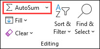
When you click AutoSum, Excel automatically enters a formula (that uses the SUM function) to sum the numbers.
Note: You can also type ALT+= (Windows) or ALT+ += (Mac) into a cell, and Excel automatically inserts the SUM function.
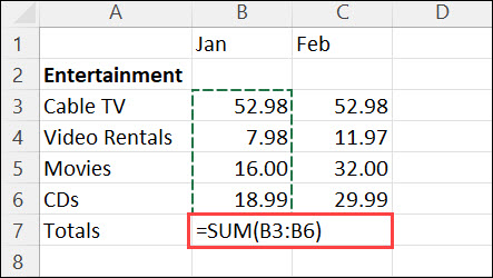
Here’s an example. To add the January numbers in this Entertainment budget, select cell B7, the cell immediately below the column of numbers. Then click AutoSum. A formula appears in cell B7, and Excel highlights the cells you’re totaling.
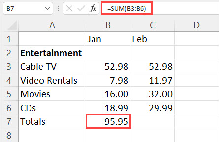
Press Enter to display the result (95.94) in cell B7. You can also see the formula in the formula bar at the top of the Excel window.
Notes:
-
To sum a column of numbers, select the cell immediately below the last number in the column. To sum a row of numbers, select the cell immediately to the right.
-
Once you create a formula, you can copy it to other cells instead of typing it over and over. For example, if you copy the formula in cell B7 to cell C7, the formula in C7 automatically adjusts to the new location, and calculates the numbers in C3:C6.
-
You can also use AutoSum on more than one cell at a time. For example, you could highlight both cell B7 and C7, click AutoSum, and total both columns at the same time.
Copy the example data in the following table, and paste it in cell A1 of a new Excel worksheet. If you need to, you can adjust the column widths to see all the data.
Note: For formulas to show results, select them, press F2, and then press Enter (Windows) or Return (Mac).
|
Data |
||
|
2 |
||
|
5 |
||
|
Formula |
Description |
Result |
|
=A2+A3 |
Adds the values in cells A1 and A2 |
=A2+A3 |
|
=A2-A3 |
Subtracts the value in cell A2 from the value in A1 |
=A2-A3 |
|
=A2/A3 |
Divides the value in cell A1 by the value in A2 |
=A2/A3 |
|
=A2*A3 |
Multiplies the value in cell A1 times the value in A2 |
=A2*A3 |
|
=A2^A3 |
Raises the value in cell A1 to the exponential value specified in A2 |
=A2^A3 |
|
Formula |
Description |
Result |
|
=5+2 |
Adds 5 and 2 |
=5+2 |
|
=5-2 |
Subtracts 2 from 5 |
=5-2 |
|
=5/2 |
Divides 5 by 2 |
=5/2 |
|
=5*2 |
Multiplies 5 times 2 |
=5*2 |
|
=5^2 |
Raises 5 to the 2nd power |
=5^2 |
Need more help?
You can always ask an expert in the Excel Tech Community or get support in the Answers community.
Need more help?
Formulas are the life and blood of Excel spreadsheets. And in most cases, you don’t need the formula in just one cell or a couple of cells.
In most cases, you would need to apply the formula to an entire column (or a large range of cells in a column).
And Excel gives you multiple different ways to do this with a few clicks (or a keyboard shortcut).
Let’s have a look at these methods.
By Double-Clicking on the AutoFill Handle
One of the easiest ways to apply a formula to an entire column is by using this simple mouse double-click trick.
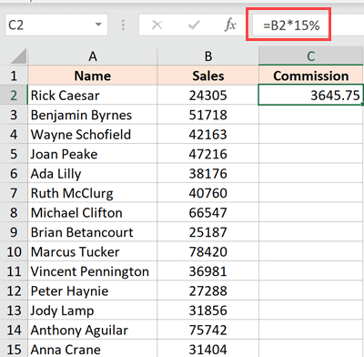
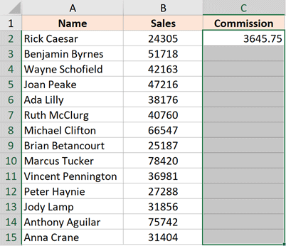
Suppose you have the dataset as shown below, where want to calculate the commission for each sales rep in Column C (where the commission would be 15% of the sale value in column B).
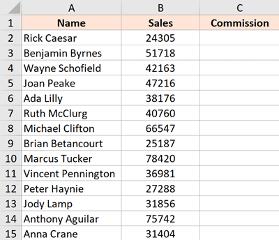
The formula for this would be:
=B2*15%
Below is the way to apply this formula to the entire column C:
- In cell A2, enter the formula: =B2*15%

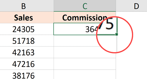
- With the cell selected, you will see a small green square at the bottom-right part of the selection.

- Place the cursor over the small green square. You will notice that the cursor changes to a plus sign (this is called the autofill handle)

- Double click the left mouse key

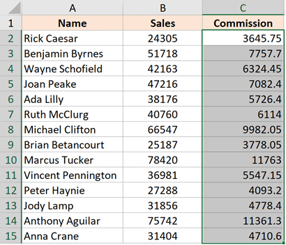
The above steps would automatically fill the entire column till the cell where you have the data in the adjacent column. In our example, the formula would be applied till cell C15
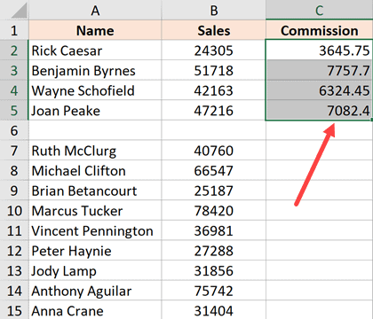
For this to work, there shouldn’t be data in the adjacent column and there should not be any blank cells in it. If, for example, there is a blank cell in column B (say cell B6), then this auto-fill double click would only apply the formula till cell C5
When you use the autofill handle to apply the formula to the entire column, it’s equivalent to copy-pasting the formula manually. This means that the cell reference in the formula would change accordingly.
For example, if it’s an absolute reference, it would remain as is while the formula is applied to the column, add if it’s a relative reference, then it would change as the formula is applied to the cells below.
By Dragging the AutoFill Handle
One issue with the above double click method is that it would stop as soon as it encountered a blank cell in the adjacent columns.
If you have a small data set, you can also manually drag the fill handle to apply the formula in the column.
Below are the steps to do this:
- In cell A2, enter the formula: =B2*15%
- With the cell selected, you will see a small green square at the bottom-right part of the selection
- Place the cursor over the small green square. You will notice that the cursor changes to a plus sign
- Hold the left mouse key and drag it to the cell where you want the formula to be applied
- Leave the mouse key when done
Using the Fill Down Option (it’s in the ribbon)
Another way to apply a formula to the entire column is by using the fill down option in the ribbon.
For this method to work, you first need to select the cells in the column where you want to have the formula.
Below are the steps to use the fill down method:
- In cell A2, enter the formula: =B2*15%
- Select all the cells in which you want to apply the formula (including cell C2)

- Click the Home tab

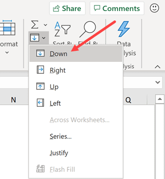
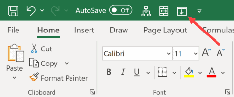
- In the editing group, click on the Fill icon

- Click on ‘Fill down’

The above steps would take the formula from cell C2 and fill it in all the selected cells
Adding the Fill Down in the Quick Access Toolbar
If you need to use the fill down option often, you can add that to the Quick Access Toolbar, so that you can use it with a single click (and it’s always visible on the screen).
T0 add it to the Quick Access Toolbar (QAT), go to the ‘Fill Down’ option, right-click on it, and then click on ‘Add to the Quick Access Toolbar’
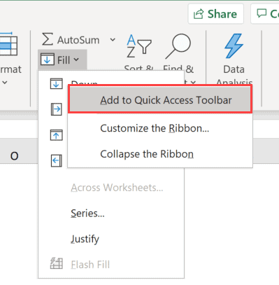
Now, you will see the ‘Fill Down’ icon appear in the QAT.
Using Keyboard Shortcut
If you prefer using the keyboard shortcuts, you can also use the below shortcut to achieve the fill down functionality:
CONTROL + D (hold the control key and then press the D key)
Below are the steps to use the keyboard shortcut to fill-down the formula:
- In cell A2, enter the formula: =B2*15%
- Select all the cells in which you want to apply the formula (including cell C2)
- Hold the Control key and then press the D key
Using Array Formula
If you’re using Microsoft 365 and have access to dynamic arrays, you can also use the array formula method to apply a formula to the entire column.
Suppose you have a data set as shown below and you want to calculate the Commission in column C.
Below is the formula that you can use:
=B2:B15*15%
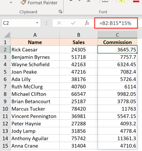
This is an Array formula that would return 14 values in the cell (one each for B2:B15). But since we have dynamic arrays, the result would not be restricted to the single-cell and would spill over to fill the entire column.
Note that you cannot use this formula in every scenario. In this case, because our formula uses the input value from an adjacent column and as the same length of the column in which we want the result (i.e., 14 cells), it works fine here.
But if this is not the case, this may not be the best way to copy a formula to the entire column
By Copy-Pasting the Cell
Another quick and well-known method of applying a formula to the entire column (or selected cells in the entire column) is to simply copy the cell that has the formula and paste it over those cells in the column where you need that formula.
Below are the steps to do this:
- In cell A2, enter the formula: =B2*15%
- Copy the cell (use the keyboard shortcut Control + C in Windows or Command + C in Mac)
- Select all the cells where you want to apply the same formula (excluding cell C2)
- Paste the copied cell (Control + V in Windows and Command + V in Mac)
One difference between this copy-paste method and all the methods convert below above this is that with this method you can choose to only paste the formula (and not paste any of the formattings).
For example, if cell C2 has a blue cell color in it, all the methods covered so far (except the array formula method) would not only copy and paste the formula to the entire column but also paste the formatting (such as the cell color, font size, bold/italics)
If you want to only apply the formula and not the formatting, use the steps below:
- In cell A2, enter the formula: =B2*15%
- Copy the cell (use the keyboard shortcut Control + C in Windows or Command + C in Mac)
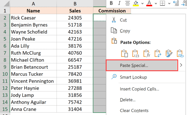
- Select all the cells where you want to apply the same formula
- Right-click on the Selection
- In the options that appear, click on ‘Paste Special’

- In the ‘Paste Special’ dialog box, click on the Formulas option

- Click OK
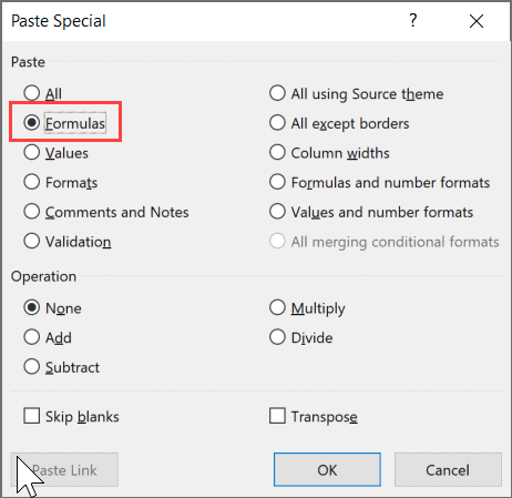
The above steps would make sure that only the formula is copied to the selected cells (and none of the formattings comes over with it).
So these are some of the quick and easy methods that you can use to apply a formula to the entire column in Excel.
I hope you found this tutorial useful!
Other Excel tutorials you may also like:
- 5 Ways to Insert New Columns in Excel (including Shortcut & VBA)
- How to Sum a Column in Excel
- How to Compare Two Columns in Excel (for matches & differences)
- Lookup and Return Values in an Entire Row/Column in Excel
- How to Copy and Paste Columns in Excel?
- Apply Conditional Formatting Based on Another Column in Excel
- How to Multiply a Column by a Number in Excel
Содержание
- Способ 1: Кнопка «Вставка функции»
- Способ 2: Вкладка «Формулы»
- Способ 3: Ручное создание формулы
- Способ 4: Вставка математической формулы
- Вопросы и ответы

Способ 1: Кнопка «Вставка функции»
Вариант с использованием специально кнопки для вызова меню «Вставка функции» подойдет начинающим юзерам и тем, кто не хочет вручную записывать каждое условие, соблюдая специфику синтаксиса программы.
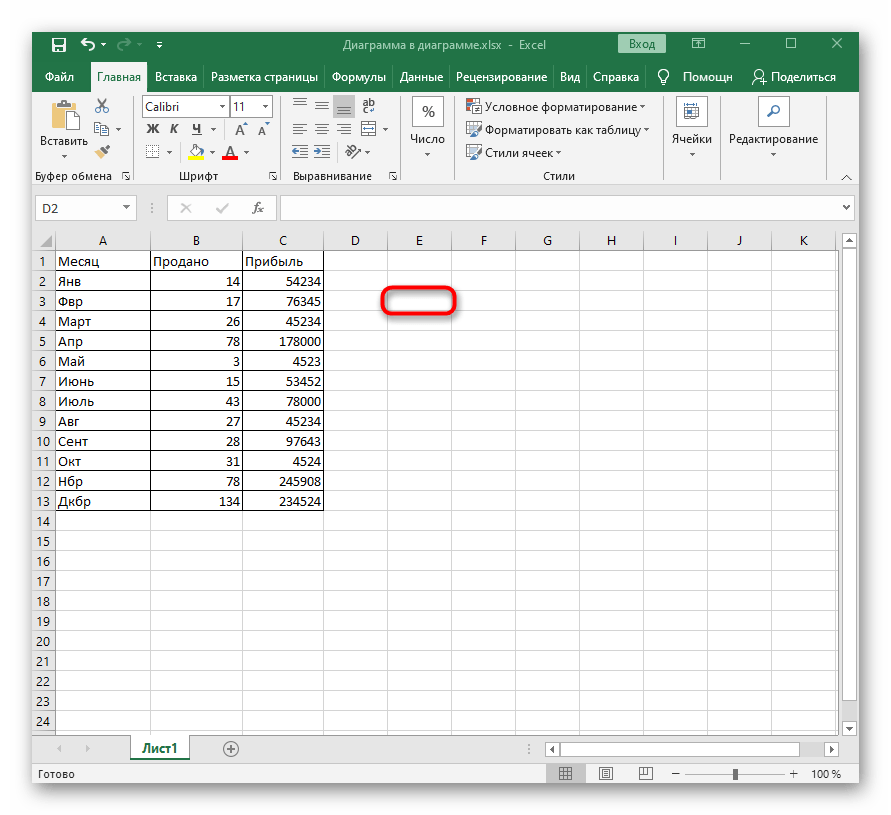
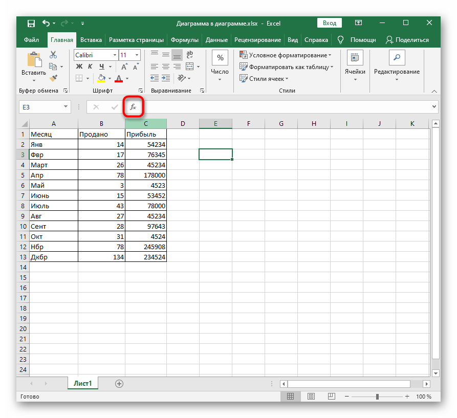
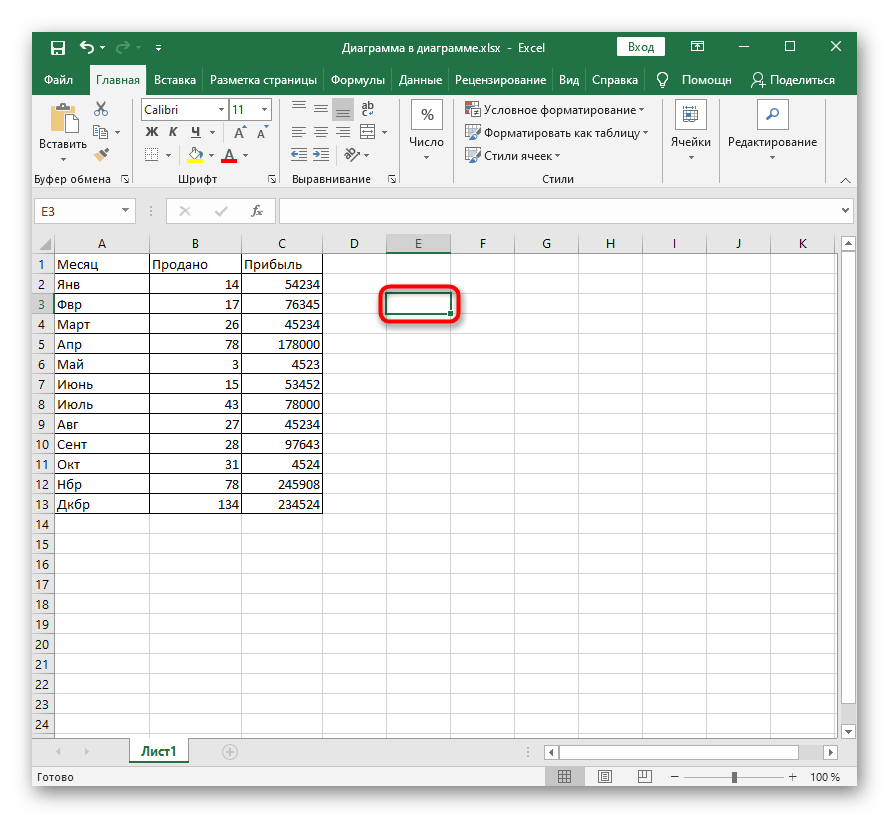
- При вставке формулы всегда в первую очередь выбирается ячейка, где в дальнейшем будет располагаться конечное значение. Сделайте это, нажав по подходящему блоку ЛКМ.
- Затем переходите к инструменту «Вставка функции» путем клика по отведенной для этого кнопке на верхней панели.
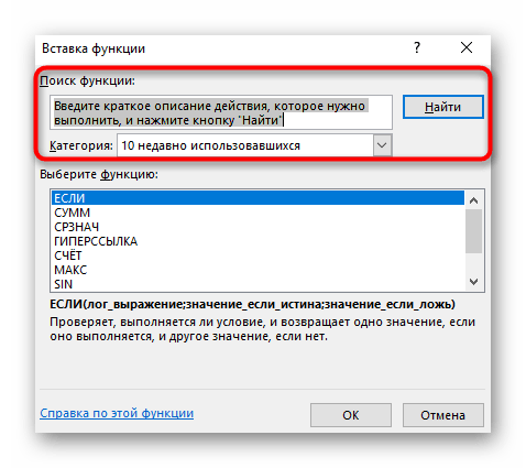
- Далее требуется отыскать подходящую функцию. Для этого можно ввести ее краткое описание или определиться с категорией.
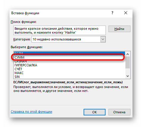
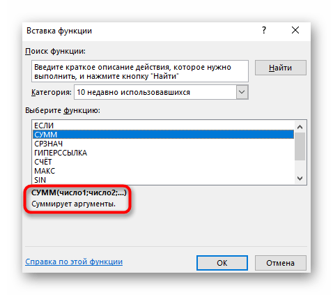
- Посмотрите на список в блоке ниже, чтобы выбрать там ту самую функцию.
- При ее выделении внизу отобразится краткая информация о действии и принцип записи.
- Для получения развернутой информации от разработчиков понадобится нажать по выделенной надписи «Справка по этой функции».
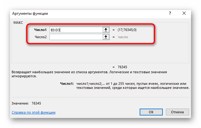
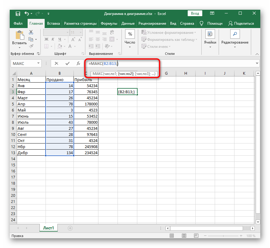
- Как только произойдет выбор функции, отобразится отдельное окно, где заполняются ее аргументы. За пример мы взяли формулу МАКС, показывающую максимальное значение из всего списка аргументов. Поэтому в качестве числа здесь задается перечень ячеек, входящих в диапазон для подсчета.
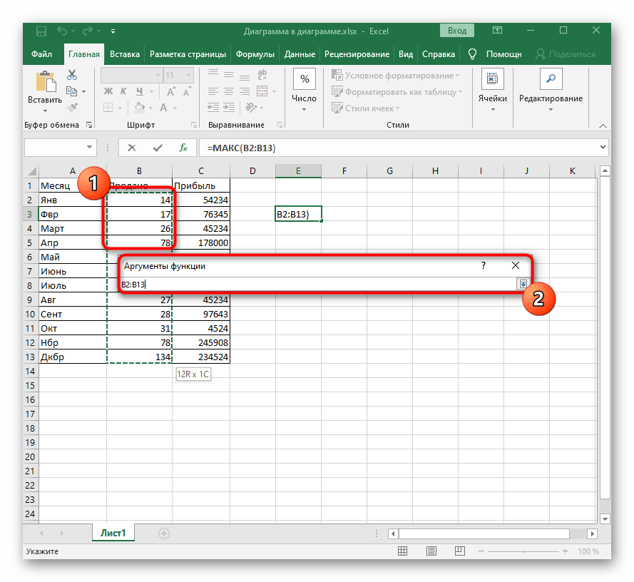
- Вместо ручного заполнения можно нажать по таблице и выделить все ячейки, которые должны попасть в тот самый диапазон.
- МАКС, как и другие функции, например самая распространенная СУММ, может включать в себя несколько списков аргументов и вычислять значения из всех них. Для этого заполняйте в таком же порядке идущие следом блоки «Число2», «Число3» и т. д.
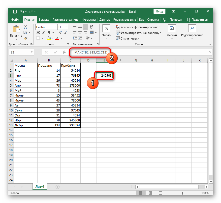
- После нажатия по кнопке «ОК» или клавише Enter формула вставится в выделенную ранее ячейку с уже отобразившимся результатом. При нажатии по ней на верхней панели вы увидите синтаксическую запись формулы и по необходимости сможете ее отредактировать.


Способ 2: Вкладка «Формулы»
Начать работу с инструментов для вставки формул, который был рассмотрен выше, можно не только при помощи нажатия по кнопке создания функции, но и в отдельной вкладке, где есть другие интересные инструменты.
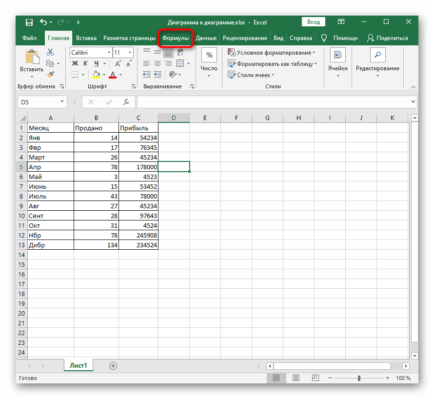
- Перейдите на вкладку «Формулы» через верхнюю панель.
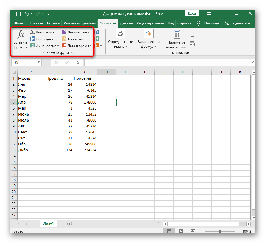
- Отсюда можно открыть упомянутое ранее окно «Вставить функцию», чтобы начать ее создание, выбрать формулу из библиотеки или воспользоваться инструментом «Автосумма», который и предлагаем рассмотреть.
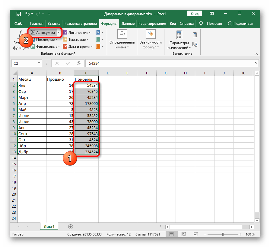
- Потребуется выделить все ячейки, которые должны суммироваться, а затем нажать по строке «Автосумма».
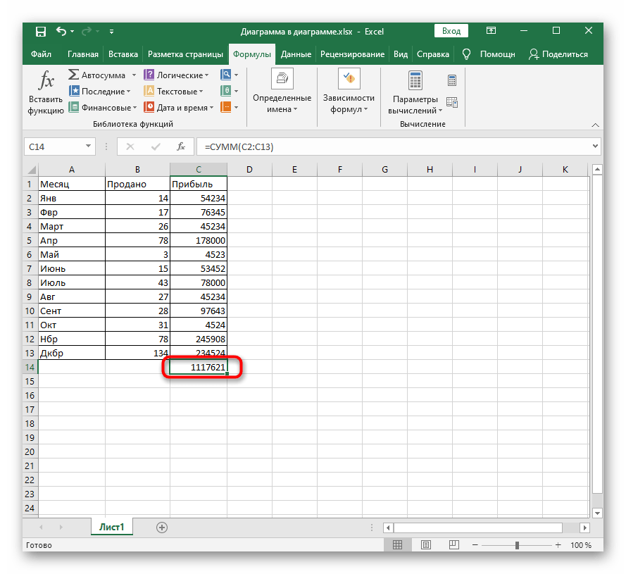
- Формула вставится автоматически со всеми аргументами, а результат отобразится в конце блока ячеек, попавших в диапазон.

Способ 3: Ручное создание формулы
Иногда проще воспользоваться ручным методом вставки формул, поскольку Мастер создания может не справиться с поставленной задачей, например, когда речь идет о большом количестве условий в ЕСЛИ или других распространенных функциях. В таких случаях заполнить ячейку самостоятельно быстрее и легче.
- Как уже было сказано в первом способе, для начала выделите ячейку, где должна располагаться формула.
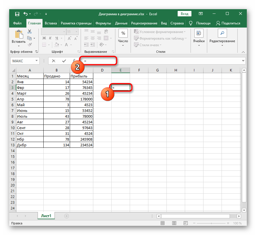
- Напишите знак «=» в поле ввода вверху или в самой ячейке, что и будет означать начало формулы.
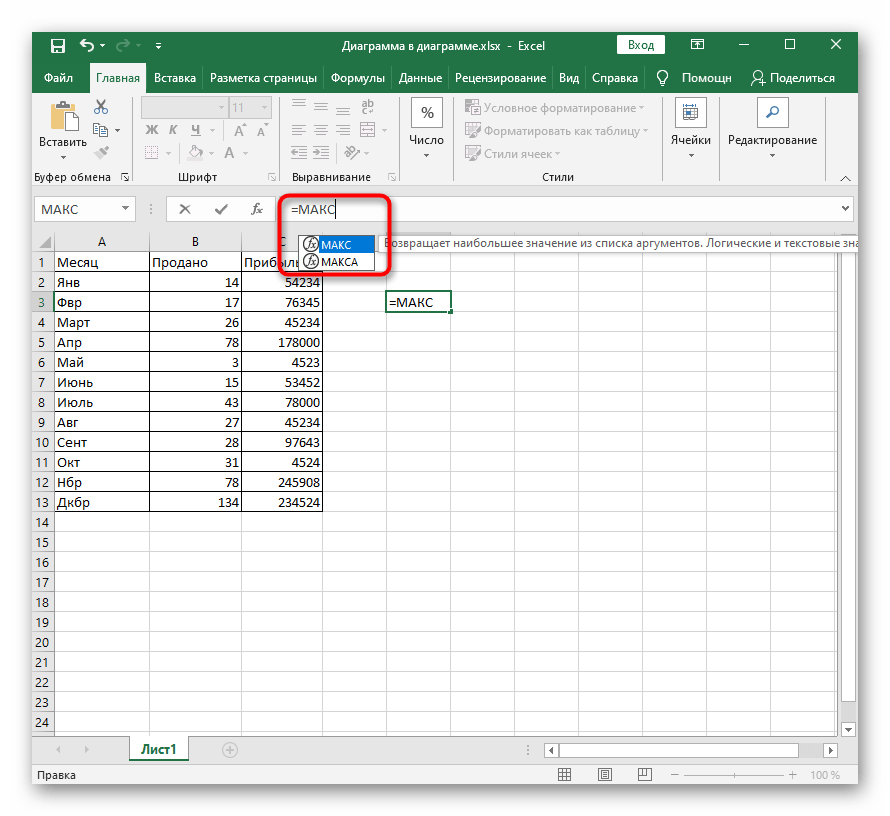
- Затем задайте саму функцию, написав ее название. Используйте подсказки для обеспечения правильности написания, а также ознакомьтесь с появившимися описаниями, чтобы определить назначение функции.
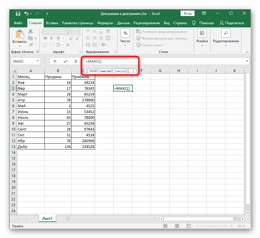
- Поставьте открывающую и закрывающую скобку, внутри которых и будут написаны условия.
- Выделите область значений или запишите ячейки, входящие в аргументы, самостоятельно. При необходимости ставьте знаки равенства или неравенства и сравнительные степени.
- Результат формулы отобразится после нажатия по клавише Enter.
- Если используется несколько рядов или аргументов, ставьте знак «;», а затем вписывайте следующие значения, что и описано в отображающихся на экране подсказках.


В завершение трех методов отметим о наличии отдельной статьи на нашем сайте, где автор разбирает большинство полезных функций, присутствующих в Excel. Если вы только начинаете свое знакомство с этой программой, посмотрите правила использования таких опций.
Подробнее: Полезные функции в Microsoft Excel
Способ 4: Вставка математической формулы
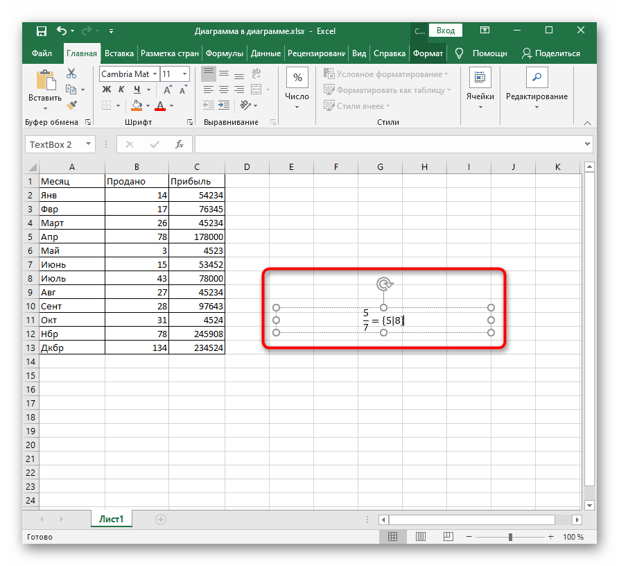
Последний вариант — вставка математической формулы или уравнения, что может пригодится всем тем пользователям, кто нуждается в создании подобных выражений в таблице. Для этого проще всего использовать специальный инструмент.
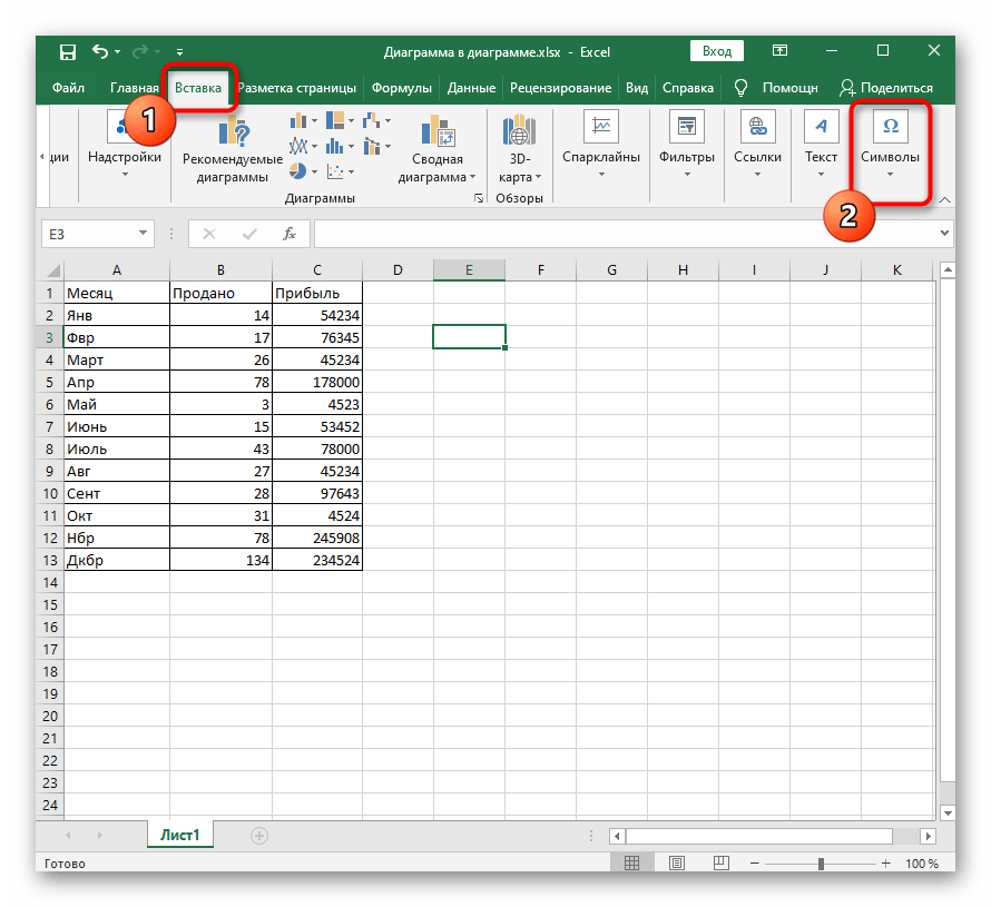
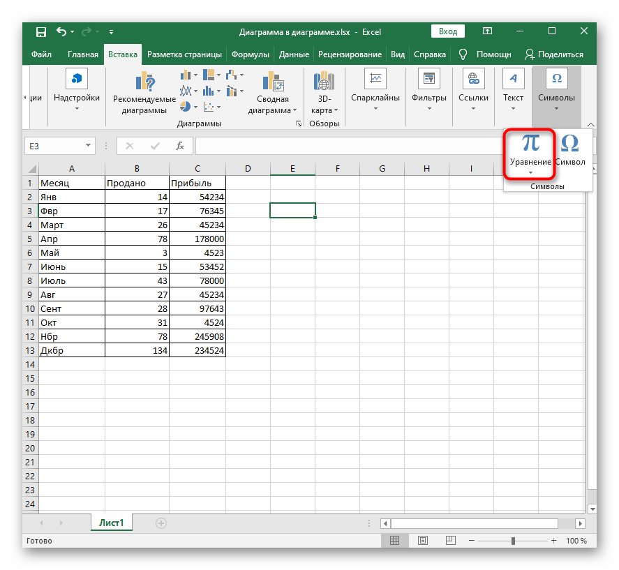
- Откройте вкладку «Вставка» и разверните раздел «Символы».
- Начните создание формулы, щелкнув по кнопке «Уравнение».
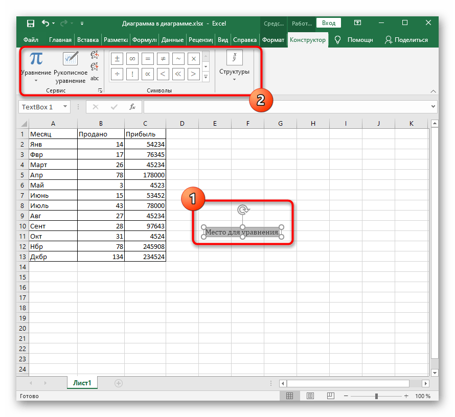
- Активируйте место для уравнения, сразу измените его размер для удобства, а затем используйте символы или готовые структуры, чтобы упростить создание формул.
- По завершении можно перемещать формулу в любое место и изменять ее внешние параметры.
Если по каким-то причинам возникли трудности с вычислением формул, скорее всего, были допущены ошибки при их вводе или появились другие неполадки. Разберитесь с этим при помощи следующей инструкции.
Подробнее: Проблемы с вычислением формул в Microsoft Excel
Еще статьи по данной теме:
Помогла ли Вам статья?

How to Create a Simple Formula in Excel
To create a formula in excel must start with the equal sign “=”. If there is no equals sign, then whatever is typed in the cell will not be regarded as a formula.
Here’s how to create a simple formula, which is a formula for addition, subtraction, multiplication, and division. An addition formula using the plus sign “+”, subtraction formula using the negative sign “-“, a multiplication formula using an asterisk sign “*” and division formula using the slash “/”.
Addition Formula
There are two numbers in cell B1 and B2. How to create a formula in excel to add both of them?

There are several ways of writing a formula. The first way is using the keyboard and the arrow keys, the second way using the keyboard and mouse and a third way to use the keyboard by typing directly the formula and the address of cell involved.
For the above addition, the formula will be used the first way.
- Place the cursor in cell B4 and then type the equals sign “=”

- Press the up arrow button, point to cell B1, the cursor turns into dashed line.

- Type the plus sign “+” for the addition operation

- Press the up arrow button again, point to cell B2

- Press the ENTER key
The result is as shown below

Subtraction Formula
How to write a formula in excel for subtracting number1 by number2?. The reduction formula to use the second way, i.e. using the keyboard and mouse.
- Place the cursor in cell B5 and then type the equals sign “=”
- Click cell B1 using the mouse
- Type the negative sign “-” for the subtraction operation
- Click cell B2 using the mouse
- Press the ENTER key
For more details, you can see the animation below.
Multiplication Formula
How to make a formula in excel to multiply number1 by number2. For the multiplication formula using the third way of using the keyboard by writing directly the formula and the address of the cell involved.
- Place the cursor in cell B6 and then type the equals sign “=”
- Type B1
- Type an asterisk “*” for multiplication operations
- Type B2
- Press the ENTER key
For more details, you can see the animation below.
Division Formula
How to do formulas in excel to divide number1 with number2.
- Place the cursor in cell B7 and then type the equals sign “=”
- Point the cursor to cell B1
- Type a slash mark “/” for the division operation
- Point the cursor to cell B2
- Press the ENTER key
The result is as shown below

How to View Formulas in Excel
The easiest way to see the formula in a cell is to look at the formula bar. Point the cursor to a cell that contains a formula, then the formula bar will display the formula in the cell. The location of the formula bar is below the ribbon menu.

The picture above shows the formula contained in cell B4. To see formulas in other cells just move the cursor to the desired cell and see the formula in the formula bar.
Formula bar can only display formulas in the active cell, meaning only one formula can be shown. To be able to display all the formulas in a worksheet, please read the article below “How to Display Cell Formulas in Excel”
How to Edit Formula in Excel
There are two ways to edit a formula, using the F2 key or using a formula bar.
Editing with the F2 key
Place the cursor in the cell containing the formula, then press the F2 key. The contents of the formula will appear, and the cells involved in the formula will be marked with a colored box.
The picture below shows the existing addition formula in cell B4. There are two cells involved in the formula: cell B1 and B2. The address of the cell B1 light blue colored then the cell B1 will be surrounded with the same colored line, likewise with cell B2, the color of lines around it is same as cell B2 address color.

For example, the formula will be edited by adding the number 2. Type the plus sign “+”, number 2 and then press the ENTER key.
The results are as shown below. The formula in cell B4 has changed.

Editing with the formula bar
Place the cursor in the cell containing the formula, then click on the formula bar section. The formula in the cell will appear automatically. The display will be the same as when pressing the F2 key.
The picture below shows the existing subtraction formula in cell B5. For example, the formula will be edited by subtracting the number 2. Type a negative sign “-” number 2, then press the ENTER key.
How to Copy Formula in Excel
The cell that contains the formula can be copied like any other data. The difference, which is copied is the formula, not the value of the cell and the cell address forming the formula will be changed according to the location.
See image below. Cell B4 contains a formula that adds the value of cell B1 and B2. The formula will be copied and placed in the range C4: F4.

Place the cursor in cell B4. Do a copy (CTRL + C). Select C4: F4 range, then paste it (CTRL + V).
The result is as shown below.

The value of cell C4 to F4 is not equal to the value of cell B4, because excel copied the formula, not the cell value. Cell C4 contains a formula that adds C1 and C2 values, as well as cell D4 until F4; all contain a formula that adds cell values in row 1 and row 2 in the same column.
Another way to copy formula in excel
In addition to using the keyboard, there is another way to copy the formula, which is using the mouse. Eg formula in cell B5 will be copied. Click cell B5, point mouse to bottom right of cell B5 until the cursor change shape become thinner. Click and hold, then drag the cursor until cell F5. The result is as shown below.
Is there any other way to copy the formula with the mouse, of course 😊. For example, the formula in range B6: B7 will be copied. Select range B6: B7, then right click select copy. Select range C6: F7, right click, select Paste. The result as shown below.
How to Paste Special in Excel
If the cell that contains the formula is copied, the formulas are copied, not its value. The question is what if you want to copy the value, not the formulas. The solution is using Paste Special.
For example, there are data like the image above. Range A4:F7 mostly contains the formula, what if the range is copied and placed on the range A9:F11?.
Select range A4:F7. Do a copy (CTRL+C). Place the cursor in cell A9, and then do a paste (CTRL + V). The results are as shown below.

The results are different. If checked, cell B9 contains formula =B6+B7, as well as other cells in range B9:F12, all containing formulas.
For copying its value only. Select range A4:F7. Do a copy (CTRL+C). Place the cursor in cell A9, and then do a paste special (CTRL+ALT+V). A dialog box appears as shown below. Select “Values”, then click OK.

The results are shown below.

The results are equal to the range A4: F7. If rechecked, the content of cell B9 and other cells in the range B9:F12 is not a formula but a number.
How to Display Cell Formulas in Excel
To see the existing formula in a cell already discussed earlier. There is one drawback, only can see the formula in one cell only. If you want to see all the formulas that exist in the worksheet, the only way is to use the “Show Formulas” command.
The location is on Ribbon Menu, Formulas tab, auditing group formula. Click once, then all data generated from formula will show its formula. Click once again; it will return to its original state.
If you want to use the Show Formulas command faster, use the shortcut CTRL + ` (grave accent, in the left position of keyboard 1 and above the left tab)
Excel is full of formulas. Those who master those formulas are pros of Excel. However, at the start of learning Excel, everyone is curious to know how to apply or create formulas in Excel. If you are one of them who is willing to learn how to create formulas in Excel, then this article is best suited for you. This article will have a complete guide from zero to intermediate level formula application in Excel.
Let us create a simple calculator-type formula for adding up numbers to start with Excel formulas.
You can download this Create a Formula Excel Template here – Create a Formula Excel Template
Look at the below data of numbers.
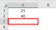
In cell A1, we have 25. The A2 cell has 40, the number.
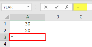
In cell A3, we need the summation of these two numbers.
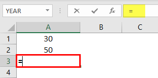
In Excel, to start the formula, always put the equal sign first.
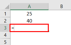
Now, insert 25 + 40 as the equation.
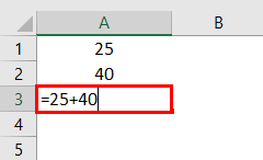
It is very similar to what we do in the calculator.
Press the “Enter” key to get the total of these numbers.

So, 25 + 40 is 65, the same we got in cell A3.
Table of contents
- How to Create a Formula in Excel?
- #1 Create Formula Flexible with Cell References
- #2 Use SUM Function to Add Up Numbers
- #3 Create Formula References to Other Cells Excel
- Recommended Articles
#1 Create Formula Flexible with Cell References
Let us start.
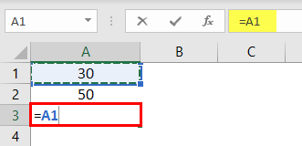
- From the above example, we will change the number from 25 to 30 and 40 to 50.

Even though we have changed numbers in cells A1 and A2, our formula only shows the old result of 65. It is a problem with direct numbers passing to the formula. It does not make the formula flexible enough to update the new result.
- We can give cell reference as the formula reference to overcoming this issue. For example, open the equal sign in cell A3.

- Then, select cell A1.

- Insert plus (+) sign and select cell A2.

- Press the “Enter” key to get the result.


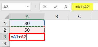
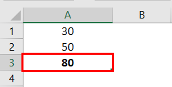
As we can see in the formula bar, it is not showing the result. Rather, it shows the formula itself, and cell A3 shows the result of the formula.
Now, we can change the numbers in A1 and A2 cells to see the immediate impact of the formula.
#2 Use SUM Function to Add Up Numbers
To get used to the formulas in Excel, let us start with the simple SUM function. All the formulas should begin with “+” or “=.” So, open the equal sign in cell A3.
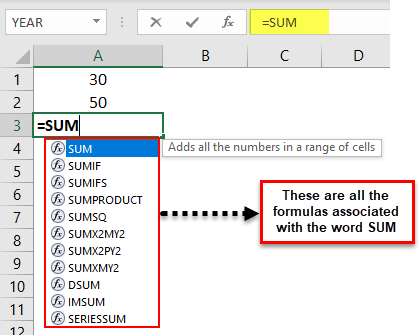
Start typing the SUM to see the intellisense list of Excel functionsExcel functions help the users to save time and maintain extensive worksheets. There are 100+ excel functions categorized as financial, logical, text, date and time, Lookup & Reference, Math, Statistical and Information functions.read more.
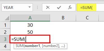
Press the “Tab” key once the SUM formula is selected to open the SUM function in excel.The SUM function in excel adds the numerical values in a range of cells. Being categorized under the Math and Trigonometry function, it is entered by typing “=SUM” followed by the values to be summed. The values supplied to the function can be numbers, cell references or ranges.read more
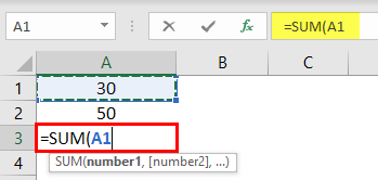
The first argument of the SUM function is Number 1, whichis the first number we need to add. In this example, cell A1. So, we must select cell A1.
The next argument is Number 2, the second number or item we need to add, A2 cell.
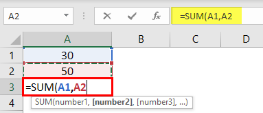
Now, we must close the bracket and press the “Enter” key to see the result of the SUM function.
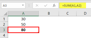
Like this, we can create simple formulas in Excel to do the calculations.
#3 Create Formula References to Other Cells Excel
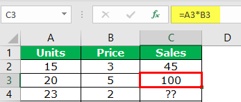
We have seen the basics of creating a formula in Excel. Similarly, we can apply one formula to other related cells as well. For example, look at the below data.
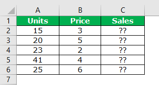
In column A we have “Units.” In column B, we have the “Price Per Unit.”
In the column, C needs to arrive at “Sales Amount.” For arriving at the sales amount, the formula is Units * Price.
- So, we must open an equal sign in cell C2.
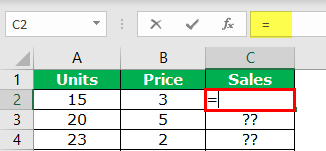
- Select cell A2 (units).
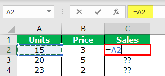
- Enter multiple sign (*) and select the B2 cell (price).
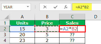
- Press the “Enter” key to get the sales amount.
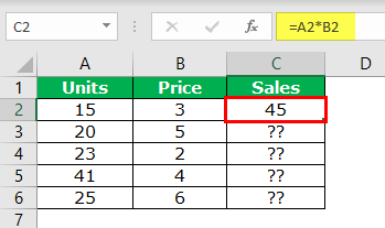
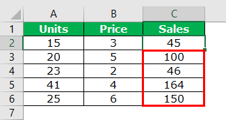
Now, we have applied the formula in cell C2. How about the remaining cells?
Can you enter the same formula for the remaining cells individually?
If you think that way, you will be delighted to hear that the “formula is to be applied to a single cell, then we can copy-paste to other cells.”
Now first, look at the formula we have applied.
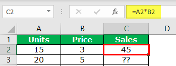
The formula says A2 * B2.
So, when we copy and paste the formula below, cell A2 becomes A3, and B2 becomes B3.
Similarly, row numbers keep changing as we move down, and column letters will also change if we move either left or right.
- Copy and paste the formula to other cells to result in all the cells.
Like this, we can create a simple formula in Excel to start your learning.
Recommended Articles
This article has been a guide to creating a formula in Excel. Here, we learn to create a simple Excel formula and practical examples, and a downloadable template. You may learn more about Excel from the following articles: –
- Write Formula in Excel
- PI in Excel
- Excel Formula Not Working
- List of Basic Excel Formulas