
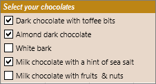
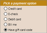
You can insert form controls such as check boxes or option buttons to make data entry easier. Check boxes work well for forms with multiple options. Option buttons are better when your user has just one choice.
To add either a check box or an option button, you’ll need the Developer tab on your Ribbon.
Notes: To enable the Developer tab, follow these instructions:
-
In Excel 2010 and subsequent versions, click File > Options > Customize Ribbon , select the Developer check box, and click OK.
-
In Excel 2007, click the Microsoft Office button
 > Excel Options > Popular > Show Developer tab in the Ribbon.
 > Excel Options > Popular > Show Developer tab in the Ribbon.
-
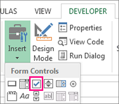
To add a check box, click the Developer tab, click Insert, and under Form Controls, click
.
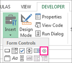
To add an option button, click the Developer tab, click Insert, and under Form Controls, click
.
-
Click in the cell where you want to add the check box or option button control.
Tip: You can only add one checkbox or option button at a time. To speed things up, after you add your first control, right-click it and select Copy > Paste.
-
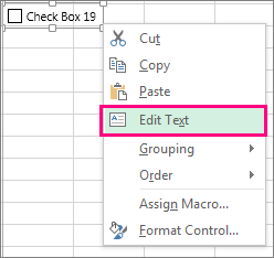
To edit or remove the default text for a control, click the control, and then update the text as needed.
 .
.
 .
.
Tip: If you can’t see all of the text, click and drag one of the control handles until you can read it all. The size of the control and its distance from the text can’t be edited.
Formatting a control
After you insert a check box or option button, you might want to make sure that it works the way you want it to. For example, you might want to customize the appearance or properties.
Note: The size of the option button inside the control and its distance from its associated text cannot be adjusted.
-
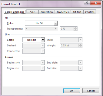
To format a control, right-click the control, and then click Format Control.
-
In the Format Control dialog box, on the Control tab, you can modify any of the available options:
-
Checked: Displays an option button that is selected.
-
Unchecked: Displays an option button that is cleared.
-
In the Cell link box, enter a cell reference that contains the current state of the option button.
The linked cell returns the number of the selected option button in the group of options. Use the same linked cell for all options in a group. The first option button returns a 1, the second option button returns a 2, and so on. If you have two or more option groups on the same worksheet, use a different linked cell for each option group.
Use the returned number in a formula to respond to the selected option.
For example, a personnel form, with a Job type group box, contains two option buttons labeled Full-time and Part-time linked to cell C1. After a user selects one of the two options, the following formula in cell D1 evaluates to «Full-time» if the first option button is selected or «Part-time» if the second option button is selected.
=IF(C1=1,»Full-time»,»Part-time»)
If you have three or more options to evaluate in the same group of options, you can use the CHOOSE or LOOKUP functions in a similar manner.
-
-
Click OK.
Deleting a control
-
Right-click the control, and press DELETE.
Currently, you can’t use check box controls in Excel for the web. If you’re working in Excel for the web and you open a workbook that has check boxes or other controls (objects), you won’t be able to edit the workbook without removing these controls.
Important: If you see an «Edit in the browser?» or «Unsupported features» message and choose to edit the workbook in the browser anyway, all objects such as check boxes, combo boxes will be lost immediately. If this happens and you want these objects back, use Previous Versions to restore an earlier version.
If you have the Excel desktop application, click Open in Excel and add check boxes or option buttons.
When we mention buttons in Excel, anyone who is not a consistent user will wonder what that means. Yes, Microsoft Excel does have Macros buttons which are the most advanced level of Excel. These buttons are commands initiated by a single click. It is easy to add buttons to excel. A user can simplify and save the time that they will take to navigate between different cells looking for specific information. In short, the buttons are inserted to perform specific tasks for us. The three different types of buttons you can place in a worksheet include;
- Shapes
- Form Control Buttons
This article shows how to add a button in Excel and how to assign Macros to them. With those buttons, navigating through your spreadsheet won’t be a nightmare anymore.
Method 1: Using shapes to create Macro buttons to open a particular sheet
You can create a macros button by using shapes. You can easily create a rounded rectangle; add a hyperlink to it for your worksheet. Here is what you can do;
1. On the main menu ribbon, click on the Insert tab.

2. Go to Shapes, click the drop-down arrow, and select the Rounded Rectangle icon.

3. Draw a rounded rectangle on your worksheet.

5. Format the shape by typing text into it-Right-click on the form and select edit text. Or double-click the shape.

6. To Hyperlink the shape, right-click on it and select Hyperlink from the menu. Right-clicking will display an Insert Hyperlink dialogue box.
- Under the ‘Link to’ section, select ‘Place in This Document.
- Under the ‘Type the cell reference’ section, type in the destination cell address.
- Under the ‘Or select a place in this document box, click to choose the particular sheet name. Click the OK button when done.
When you click the rounded rectangle, it will skip to the specified cell of a specified sheet.

7. To assign the macro, right-click on the table and select Assign Macro. Under the ‘Macros in’ drop-down arrow, select ‘This Workbook’. Here, select the macro from the list of macros in This Workbook.

8. Press OK. When you point your mouse on this shape, it will turn to the hand pointer cursor, and clicking the form will run the macro. Remember to set your shape not to resize with cell changes by right-clicking on it and selecting ‘Size and Properties.’
Method 2: Using Developers Form Control Buttons to create buttons in Excel
1. On the main ribbon, click on the Developer tab.
2. Go to the Insert button and click the drop-down arrow.

3. Under Form Control, select the first option called button. Draw a button on your worksheet

4. Next, in the Assign Macro dialogue box, type or select a name for the macro.

5. Click OK when done. You can click on this button to run the macro.

Using ActiveX Controls
Since running a macro in Excel can prove tedious, you can assign a macro to a button to run it faster. In this case, you can follow these steps to add a button in Excel using ActiveX controls easily.
1. Right-click anywhere on the Home ribbon and select Customize the Ribbon option from the pop-up menu.
2. Once the Customize the Ribbon window is open, go to the Main Tabs section and select the Developer option.
3. Click OK. However, if you already have the Developer Tab added to your ribbon, then proceed as follows.
4. Go to the Developer Tab and click on Insert.

5. Next, click on your preferred button under the ActiveX Controls.

You can now drag it anywhere in the Excel worksheet to create a button.
6. Right-click on the newly created button and select the View Code option from the drop-down menu.

7. You can now type this code, which sets the value of cell A6 to Hello:
Range(“A6”).Value = “Hello”

8. If you want to test setting the cell value, ensure the Design Mode option is deselected. You can also click on the button, and the Hello text will be displayed on your screen.

You can further use VBA codes to assign a different task for various operations such as double-clicking, single-clicking, right-clicking, and many more. When you right-click on the button, you can also select the Format Control option. However, the only downside is that the size of the buttons changes every time you make changes on the worksheet or share it.
Adding Macros To Quick Access Toolbar
Adding macros to Quick Access Toolbar also allows you to create buttons in Excel and use them on any sheet in your present workbook. To do this, follow these steps:
1. Right-click on the arrow below the ribbon of the Excel workbook.

2. When the Customize Quick Access Toolbar screen opens, navigate and select More Commands at the bottom.

3. Select Macros in the Choose commands from the section. You can click on the down-facing arrow in the Popular Commands box.

4. Select the HighlightMaxValue option and click on the Add button.

5. You can now click on Modify to customize the symbol of the macro.

6. Select your preferred symbol from the provided list and hit the OK button.

7. Finish by clicking OK to add a button to your Excel workbook. If you want to run the HighlightMaxValue macro, simply click on the icon.
Conclusion
When working with adding buttons to Excel, it is best to keep it easy and straightforward. The above methods portray these as the steps are short and easy to follow. They are not only easy to set up, but they also give you different options for formatting.
Microsoft Excel lets you add two types of buttons to a worksheet: option buttons and toggle buttons. Option buttons, also referred to as radio buttons, let you choose one item from a list. Toggle buttons are either enabled or disabled, allowing you to switch between two states, such as on and off. Once a button is inserted into your worksheet, you then assign it form or ActiveX controls to make it perform an action when clicked.
Option Button
-
Open Excel and Click on «Developer» Tab
-
Open Excel and click on the «Developer» tab. If it’s not visible, click “File,” “Options” and then “Customize Ribbon.” Click the “Developer” check box within the Main Tabs list and click the «OK» button when you’re finished.
-
Select «Insert»
-
Select “Insert” from the Controls group on the Developer tab.
-
Choose the Type of Button
-
Click the type of option button you’d like to insert. Form Control and ActiveX Control are the two main categories. To insert a Form Control option button, click “Option Button” from the list of Form Controls. The names of the buttons appear when you hover the mouse over them. To insert an ActiveX Control option button, click “Option Button” from the list of ActiveX Controls.
-
Click the Cell on Your Worksheet
-
Click the cell on your worksheet where you want your option button displayed.
-
Format the Button
-
Format or edit your button properties to make it do something when clicked. For example, if you inserted a Form Control option button, right-click it and select “Format Control” from the drop-down menu to edit its properties. If you inserted an ActiveX Control button, right click your button and select “Properties» from the drop-down menu.
Toggle Button
-
Click «Insert» in Controls Group
-
Click “Insert” in the Controls group on the Developer tab in Excel.
-
Select «Toggle Button»
-
Select “Toggle Button” from the list of ActiveX Controls.
-
Click where Button Should Appear
-
Click your cursor in worksheet cell where you’d like the toggle button to appear.
-
Select «Properties»
-
Right-click the button and select “Properties” to assign ActiveX controls to it.
Tip
You can also assign macro controls to option buttons. With an option button inserted into your worksheet, right-click it and select “Assign Macro.” Choose the macro you’d like to use from the pop-up dialog box and then press “OK.”
Как сделать кнопку в Excel? Войдите в раздел «Разработчик», откройте меню «Вставить», выберите изображение и назначьте макрос, гиперссылку, переход на другой лист или иную функцию. Ниже подробно рассмотрим все способы создания клавиш в Эксель, а также приведем функции, которые им можно присвоить.
Как создать кнопку: базовые варианты
Перед тем как сделать кнопку в Эксель, убедитесь в наличии режима разработчика. Если такой вкладки нет, сделайте следующие шаги:
- Жмите по ленте правой клавишей мышки (ПКМ).
- В появившемся меню кликните на пункт «Настройка ленты …».
- В окне «Настроить ленту» поставьте флажок возле «Разработчик».
- Кликните «ОК».
После того, как сделана подготовительная работа, можно вставить кнопку в Excel. Для этого можно использовать один из рассмотренных ниже способов.
Через ActiveX
Основной способ, как создать кнопку в Excel — сделать это через ActiveX. Следуйте такому алгоритму:
- Войдите в раздел «Разработчик».
- Жмите на кнопку «Вставить».
- В появившемся меню выберите интересующий элемент ActiveX.
- Нарисуйте его нужного размера.

Через элемент управления
Второй вариант — создание кнопки в Excel через элемент управления. Алгоритм действий такой:
- Перейдите в «Разработчик».
- Откройте панель «Вставить».
- Выберите интересующий рисунок в разделе «Элемент управления формы».
- Нарисуйте нужный элемент.
- Назначьте макрос или другую функцию.

Через раздел фигур
Следующий способ, как добавить кнопку в Excel на лист — сделать это с помощью раздела «Фигуры». Алгоритм действий такой:
- Перейдите в раздел «Вставка».
- Войдите в меню «Иллюстрации», где выберите оптимальную фигуру.
- Нарисуйте изображение необходимой формы и размера.
- Кликните ПКМ по готовой фигуре и измените оформление.

В качестве рисунка
Вставка кнопки Excel доступна также в виде рисунка. Для достижения результата пройдите такие шаги:
- Перейдите во вкладку «Вставка».
- Кликните в категорию «Иллюстрации».
- Выберите «Рисунок».
- Определитесь с типом клавиши, который предлагается программой.

Какие кнопки можно создать
В Excel возможно добавление кнопки двух видов:
- Command Button — срабатывает путем нажатия, запускает определенное действие (указывается индивидуально). Является наиболее востребованным вариантом и может играть роль ссылки на страницу, таблицу, ячейку и т. д.
- Toggle Button — играет роль переключателя / выключателя. Может нести определенные сведения и скрывать в себе два параметра — Faste и True. Это соответствует двум состояниям — нажато и отжато.
Также перед тем как поставить кнопку в Эксель, нужно определиться с ее назначением. От этого напрямую зависят дальнейшие шаги. Рассмотрим разные варианты.
Макрос
Часто бывают ситуации, когда необходимо создать кнопку макроса в Excel, чтобы она выполняла определенные задачи. В обычном режиме для запуска нужно каждый раз переходить в раздел разработчика, что требует потери времени. Проще создать рабочую клавишу и нажимать ее по мере неободимости.
Если вы решили сделать клавишу с помощью ActiveX, алгоритм будет таким:
- Войдите в «Режим конструктора».

- Кликните дважды по ней.
- В режиме Visual Basic между двумя строками впишите команду, необходимую для вызова макроса., к примеру, Call Макрос1.

- Установите назначение для остальных графических объектов, если они есть.
Зная, как назначить кнопку в Excel, вы легко справитесь с задачей. Но можно сделать еще проще — жмите на рисунок ПКМ и в списке внизу перейдите в раздел «Назначить макрос». Здесь уже задайте интересующую команду.

Переход на другой лист / ячейку / документ
При желании можно сделать кнопку в Excel, которая будет отправлять к другому документу, ячейке или листу. Для этого сделайте следующее:
- Подготовьте клавишу по схеме, которая рассмотрена выше.
- Выделите ее.
- На вкладке «Вставка» отыщите «Гиперссылка».

- Выберите подходящий вариант. Это может быть файл, веб-страница, e-mail, новый документ или другое место.
- Укажите путь.

Рассмотренный метод не требует указания макросов и предоставляет расширенные возможности. При желании можно также использовать и макросы.
Существует и другой способ, как сделать кнопку в Excel для перехода к определенному листу. Алгоритм такой:
- Создайте рисунок по рассмотренной выше схеме.
- В окне «Назначить макрос» введите имя макроса, а после жмите на клавишу входа в диалоговое окно Microsoft Visual Basic.
- Вставьте код для перехода к другому листу — ThisWorkbook.Sheets(«Sheet1»).Activate. Здесь вместо Sheet1 укажите путь к листу с учетом запроса.
- Сохраните код и закройте окно.
Сортировка таблиц
При желании можно сделать клавишу для сортировки таблиц Excel. Алгоритм действий такой:
- Создайте текстовую таблицу.
- Вместо заголовков добавьте автофигуры, которые в дальнейшем будут играть роль клавиш-ссылок на столбцах таблицы.

- Войдите в Visual Basic режим, где в папке Modules вставьте модуль Module1.
- Кликните ПКМ по папке и жмите на Insert Module.
- Сделайте двойной клик по Module1 и введите код.
- Назначьте каждой фигуре индивидуальный макрос.

После выполнения этих шагов достаточно нажать по заголовку, чтобы таблица сортировала данные в отношении определенного столбца.
По рассмотренным выше принципам несложно разобраться, как в Экселе сделать кнопки выбора и решения других задач. В комментариях расскажите, какой из приведенных методов вам подошел, и как проще всего самому сделать клавишу в программе.
Отличного Вам дня!
Skip to content
![]()
 You are looking for a simply way to make your Excel table look professional? Hardly known but easy to use: Buttons, for example, Check Boxes or Spin Buttons can change values.
How to easily insert buttons in Excel
Before you start using buttons, you have to display the Developer tools. Right click on any ribbon and click “Customize the Ribbon”. Make sure the box for Developer is ticked on the right hand side.
To insert a Check Box (the numbers are corresponding to the picture above):
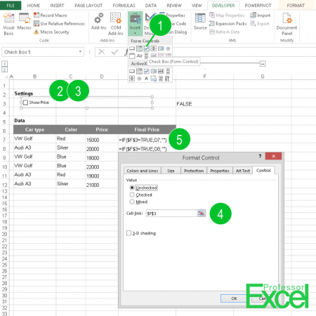
- Select the Check Box under “Insert” on the Developer ribbon.
- Place the Check Box on your Excel sheet.
- Right-click on it and go to “Format Control”.
- The Check Box needs one cell in which it writes “TRUE” or “FALSE”, depending on if it’s checked or not.
- Now you can use the specified cell in your formulas. In the above example, if cell F3 is set to TRUE, the price of the car will be shown in cell E7 (see the IF formula in cell E7).
You can use “Spin Buttons” (next to the Check Box on the Insert menu) more or less the same way. You have to define a cell. By pressing on the arrow up or down the value in that cell will be modified.

Henrik Schiffner is a freelance business consultant and software developer. He lives and works in Hamburg, Germany. Besides being an Excel enthusiast he loves photography and sports.
We use cookies on our website to give you the most relevant experience by remembering your preferences and repeat visits. By clicking “Accept”, you consent to the use of ALL the cookies.
.