How do you use formulas in excel

The Excel Formulas Ultimate Guide 

Introduction to Excel Formulas

In this guide, we are going to cover everything you need to know about Excel Formulas. Learning how to create a formula in Excel is the building block to the exciting journey to become an Excel Expert. So, let’s get started!

What is an Excel Formula?

Excel Formulas are often referred to as Excel Functions and it’s no big deal but there is a difference, a function is a piece of code that executes a predefined calculation, and a formula is an equation created by the user.

A formula is an expression that operates on values in a cell or range of cells. An example of a formula looks like this: = A2 + A3 + A4 + A5. This formula will result in the sum of the range of values from cell A2 to cell A5.

A function is a predetermined formula in Excel. It shows calculations in a particular order defined by its parameters. An example of a function is =SUM (A2, A5). This function will also provide the addition of values in the range of cells from A2 to A5 but here instead of specifying each cell address we are using the SUM function.

How To Write Excel Formulas

Let’s look at how to write a formula on MS Excel. To begin with, a formula always starts with a ‘+’ or ‘=’ sign, if you start writing the formula without any of these two signs, Excel will treat the value in that cell as text and will not perform any function.

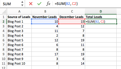
In the screenshot below, you need to calculate the total sales amount by multiplying quantity sold with unit price. Select cell D2, type the formula ‘=B2*C2’ and press Enter. The result will display on cell D2.

Apply A Formula To An Entire Column Or Range

To copy a formula to adjacent cells, you can do the following:

1. Select the cell with the formula and the adjacent cells you want to fill, then drag the fill handle.

1. Select the cell with the formula and the adjacent cells you want to fill, then press Ctrl+D to fill the formula down in a column, or Ctrl+R to fill the formula to the right in a row.
2. Select the cell with the formula and the adjacent cells you want to fill, then Click Home > Fill, and choose either Down, Right, Up, or Left.

How to Copy A Formula And Paste It

Excel allows you to copy the formula entered in a cell and paste it on to another cell, which can save both time and effort. To copy paste a formula:

1. Select the cell whose formula you wish to copy
2. Press Ctrl + C to copy the content
3. Select the cell or cells where you wish to paste the formula. The copied cells will now have a dashed box around them.
4. Press Alt + E + S to open the paste special box and select ‘Formula’ or Press “F’ to paste the formula.

1. The formula will be pasted into the selected cells.

Basic Excel Formulas

Let’s start off with simple Excel Formulas. In the screenshot below, there are two columns containing numbers and we would like to use different operators like addition, subtraction, multiplication, and division on those to get different results. Excel uses standard operators for formulas, such as a plus sign for addition (+), a minus sign for subtraction (-), an asterisk for multiplication (*), a forward slash for division (/).

• Addition– To add values in the two columns, simply type the formula =A2+B2 on cell C2 and then copy paste the same on the cells below.
• Subtraction – To subtract values in Column B from Column A, simply type the formula =B2-A2 on cell C2 and then copy paste the same on the cells below.
• Multiplication – To multiply values in the two columns, simply type the formula =A2*B2 on cell C2 and then copy paste the same on the cells below.
• Division – To divide values in Column a by values in Column B, simply type the formula =A2/B2 on cell C2 and then copy paste the same on the cells below.

We can also calculate the percentage using Excel Formulas. In the image below, we have sales in Year 1 and Year 2 and we would like to know the % growth in sales from Year 1 to Year 2.

To do that, select cell C2 and type the formula = (B2 – A2)/B2*100

Basic Excel Functions

A function is a predefined formula that performs calculations using specific values in a particular order. Excel includes many common functions that can be useful for quickly finding the sum, average, count, maximum value, and minimum value for a range of cells. a function must be written a specific way, which is called the syntax.

The basic syntax for a function is an equals sign (=), the function name, and one or more arguments. A Function is generally comprised of two components:

1) A function name -The name of a function indicates the type of math Excel will perform.

2) An argument – It is the values that a function uses to perform operations or calculations. The type of argument a function uses is specific to the function. Common arguments that are used within functions include numbers, text, cell references, and names

Let’s look at some common Excel Functions:

SUM Function

The SUM formula adds 2 or more numbers together. You can use cell references as well in this formula.

Syntax: =SUM(number1, [number2], …)

Example: =SUM(A2:A8) or SUM(A2:A7, A9, A12:A15)

AUTOSUM Function

The AutoSum command allows you to automatically insert the most common functions into your formula, including SUM, AVERAGE, COUNT, MIN, and MAX.

Select the cell where you want the formula, Go to Home > Click on AutoSum > From the dropdown click on “Sum” > Enter.

COUNT Function

If you wish to how many cells are there in a selected range containing numeric values, you can use the function COUNT. It will only count cells that contain either numbers or dates.

Syntax: =COUNT(value1, [value2], …)

In the example below, you can see that the function skips cell A6 (as it is empty) and cell A11 (as it contains text) and gives you the output 9.

COUNTA Function

Counts the number of non-empty cells in a range. It will include cells that have any character in them and only exclude blank cells.

Syntax: =COUNTA(value1, [value2], …)

In the example below, you can see that only cell A6 is not included, all other 10 cells are

counted.

AVERAGE Function

This function calculates the average of all the values or range of cells included in the parentheses.

Syntax: =AVERAGE(value1, [value2], …)

ROUND Function

This function rounds off a decimal value to the specified number of decimal points. Using the ROUND function, you can round to the right or left of the decimal point.

Syntax: =ROUND(number,num_digit)

This function contains 2 arguments. First, is the number or cell reference containing the number you want to round off and second, number of digits to which the given number should be rounded.

• If the num-digit is greater than 0, then the value will be rounded to the right of the decimal point.
• If the num-digit is less than 0, then the value will be rounded to the left of the decimal point.
• If the num-digit equal to 0, then the value will be rounded to the nearest integer.

MAX Function

 This function returns the highest value in a range of cells provided in the formula.

Syntax: =MAX(value1, [value2], …)

In the example below, we are trying to calculate the maximum value in the dataset from A2 to A13. The formula used is =MAX(A2: A13) and it returns the maximum value i.e. 96.251

MIN Function

This function returns the lowest value in a range of cells provided in the formula.

Syntax: =MIN(value1, [value2], …)

In the example below, we are trying to calculate the minimum value in the dataset from A2 to A13. The formula used is =MIN(A2: A13) and it returns the minimum value i.e. 24.178

TRIM Function

 This function removes all extra spaces in the selected cell. It is very helpful while data cleaning to correct formatting and do further analysis of the data.

Syntax: =trim(cell1)

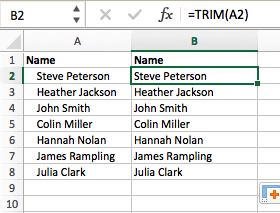
In the example below, you can see the name in cell A2 contains an extra space, in the beginning, =TRIM(A2) would return “Steve Peterson” with no spaces in a new cell.

Advanced Excel Formulas

Here is a list of Excel Formulas that we would feel comfortable referring to as the top 10 Excel Formulas. These formulas can be used for basic problems or highly advanced problems as well, though advanced excel formulas are nothing but a more creative way of using the formulas. Sure, there are legitimate Advanced Excel Formulas such as Array Formulas but in general the more advanced the problem, the more creative you need to be with Formulas.

Currently, Excel has well over 400 formulas and functions but most of them are not that useful for corporate professionals so here is a list that we believe contains the 10 best Excel formulas.

Starting with number 10 – it’s the IFERROR formula

1. IFERROR Function –
2. SUBTOTAL Function –
3. SMALL/LARGE Function –
4. LEFT Function –
5. RIGHT Function –
6. SUMIF Function –
7. MATCH Function –
8. INDEX Function –
9. VLOOKUP Function –
10. IF Function –

IFERROR Function –

You ever have presented a worksheet that you thought was perfect but were surprised with a “#DIV /0!” error or an “#N/A” error message (See the screenshot below), then this function is perfect for you. Excel has an “IFERROR” function that can automatically replace error messages with a message of your choice.

The IFERROR function has two parameters, the first parameter is typically a formula and the second parameter, value_if_error, is what you want Excel to do if value, the first parameter, results in an error. Value_if_error can be a number, a formula, a reference to another cell, or it can be text if the text is contained in quotes.

That means you can put formula or an expression in the first part of the IFERROR function and Excel will show the result of that formula unless the formula results in an error. If the formula results in an error, Excel will follow the instructions in the second half of the IFERROR formula.

This function cleans up your sheet and it will visually make things look a lot better and more professional.

Let’s see an example to make the concept clearer.

In this example, we have two lists – one contains the names of all people (Column A) and the second list contains the name of award winners only (Column F).

We have used a simple Vlookup function to see if the name is an award winner. The Vlookup function (it is covered later in details) will search the list on the right, if the name is present in the award winner list, it will show the name or else it will show an error.

The N/A error makes the worksheet look dirty and unprofessional. Now we will add iferror function here to remedy the same.

=IFERROR(VLOOKUP(A5,$F$5:$F$10,1,0),””)

IFERROR function will recognize the error and instead of displaying the error message will display the text, say a blank, or you can show any other message that you desire.

IFERROR is a great way to replace Excel-generated error messages with explanations, additional information, or simply leave the cell blank.

SUBTOTAL Function –

The SUBTOTAL function returns the aggregate value of the data provided. You can select any of the 11 functions that SUBTOTAL can calculate like SUM, COUNT, AVERAGE, MAX, MIN, etc. SUBTOTAL Function can also include or exclude values in hidden rows based on the input provided in the function.

Excel’s traditional formulas do not work on filtered data since the function will be performed on both the hidden and visible cells. To perform functions on filtered data one must use the subtotal function.

Syntax: SUBTOTAL(function_num,ref1,…)The first parameter is the name of the function to be used within the subtotal function and the second parameter is the range of cells that should be subtotalled

The list of functions that can be used in given below. If the data is filtered manually, the numbers from 1 – 11 will include the hidden cells and number from 101 – 111 will exclude them.

Let’s understand this function with an example.

Here we have a list of name of person, with their country and the total sales they have achieved in Q1. We will use the subtotal function to calculate the total sales in cell C26. We will also select the function in such a way that it works on filtered data as well.

The formula will be =SUBTOTAL (109,C5:C24)

This will display the total sales. Now, we filter the data to see the sales made by people in US only. You will see the value in the cell containing the SUBTOTAL function updates and it filters the dataset and displays the total sales made by US only.

Here is another benefit of using a SUBTOTAL function:

When you’re creating an information summary, especially like a profit and loss statement where you’ve got lots of subtotals, what you can do is you can use the subtotal formula, and then at the end, you can put a big old formula right at the end and it will just ignore your subtotal.

Here we have 4 different tables for sales in 4 different countries.

We can add individual SUBTOTAL functions for each table and then a grand total function in the end. The SUBTOTAL function in the end will ignore all the other SUBTOTAL functions above it and will provide you the total sales.

SMALL/LARGE Function –

Here, we have two formulas and they’re two sides of the same coin – the small formula and the large function. So, imagine you’ve got a list of, let’s say, sales data or cost data and what SMALL Function will do is provide you with the smallest value in the data set. You can also specify if you want the first smallest or second smallest. Similarly, with the large formula, you can extract the largest value in this dataset, the second largest and so on.

Syntax: =LARGE(array,k); SMALL(array,k)

The first parameter is the range of data for which you want to determine the k-th largest value and the second is the position (from the largest/smallest) in the cell range of the value to return.

Now, in the dataset above if you want to know the person who has achieved the highest sales, you can use the LARGE function – =LARGE($C$4:$C$23,E5). We have used E5 for the second parameter as it contains the value 1. If we copy paste the formula in the cells below, you will get the 1^st, 2^nd, 3^rd, 4^th and 5^th largest value in the dataset. Similarly, we have used the function SMALL to get the value for lowest sales.

LEFT & RIGHT Function –

A lot of people work on text manipulation with functions like text to columns or even do it manually but being able to extract the exact number of characters that you want from the left or the right side of a string is absolutely invaluable. This is what the LEFT and RIGHT function does – it extracts a given number of characters from the left/right side of a supplied text string.

Syntax: =LEFT (text, [num_chars]) and RIGHT(text,num_chars)

The first parameter is the text string containing the characters you want to extract and the second parameter specifies how many characters you want LEFT/RIGHT to extract; 1 if omitted.

In the example given below, we have full names of people and we would like to extract the first name. We can surely do it using text to column, but using the LEFT function will give us a more automated result. So, let’s see how it can be done.

When you look at the data, you can see that a character is common in all names and it separates the first name and last name – it is a “space”. If we can find out the position of space in each cell, we can easily extract the first name.

Does Excel have a formula for this as well? Off course! SEARCH is the function that will come to your rescue.

SEARCH function provides the position of the first occurrence of the specified character.SEARCH (find_text, within_text, start_num) has three parameters – first is the character you want to find, second is the text in which you want to search and third is the character number in Within_text, counting from the left, at which you want to start searching. If omitted, 1 is used.

So, going back to our example, we use the formula SEARCH to find the position of the character – space in Column A. We will need to subtract “1” from the position to get the desired result. The formula will be =SEARCH (“ “,A5)-1 and copy paste it down.

Now we will use the LEFT Function to get the first name. =LEFT(A5,B5) – A5 contains the full name and B5 contains the number of characters from left that contains the first name.

SUMIF(S) Function –

This function is used to conditionally sum up a range of values. It returns the summation of selected range of cells if it satisfies the given criteria. It is like the SUM function because it adds stuff up. But, it allows us to specify conditions for what to include in the result. Criteria can be applied to dates, numbers, and text using logical operators (>,<,<>,=) and wildcards (*,?) for partial matching. For example, SUMIF function can add up the quantity column, but only include those rows where the SKU is equal to, say A200.

Syntax: =SUMIF (range, criteria, [sum_range])

The first argument is the range of values to be tested against the given criteria, second argument is the condition to be tested against each of the values and the last argument is the range of numeric values if the criteria is satisfied. The last argument is optional and if it is omitted then values from the range argument are used instead.

SUMIF can handle one criterion only. For multiple conditional summing – we can use SUMIFS.

The Syntax of this function is =SUMIFS( sum_range, criteria_range1, criteria1, [criteria_range2, criteria2], … ); where sum_range is the range of values to add, criteria_range1 is the range that contains the values to evaluate and criteria1 is the value that criteria_range1 must meet to be included in the sum. You can add additional pairs of criteria range and criteria if further conditions are to be met.

It is advisable to use SUMIFS even if you have only one criteria to evaluate as it will help you to easily modify the function if additional conditions come up over time.

Let’s dive into an example. Below we have data containing name, country in which sales were made, and the different quarterly sales data.

Using SUMIFS function, we would like to calculate the sum of sales in Q1 for the different countries. Now, to get the total sales in UK in Q1, we select the cell I4 and type the formula =SUMIFS(C4:C23,B4:B23,H4). We will then copy paste the formula below to get the result for each country.

INDEX & MATCH Function –

The MATCH function is used to search for an item and return the relative position of that item in a horizontal or vertical list.

Syntax: MATCH(lookup_value, lookup_array, [match_type])

The first argument is the value you want to look up, second is the range of cells being searched and the last argument, which is optimal, tells the MATCH function what sort of lookup to do.

The three acceptable values for match type are 1, 0 and -1. The default value for this argument is 1.

• If the input is 1. MATCH finds the largest value that is less than or equal to the lookup_value. The values in the lookup_array argument must be placed in ascending order.
• If the input is 0. MATCH finds the first value that is exactly equal to the lookup_value. The values in the lookup_array argument can be in any order.
• If the input is -1. MATCH finds the smallest value that is greater than or equal to the lookup_value. The values in the lookup_array argument must be placed in descending order.

For example, if the range A1:A5 contains the values Evelyn Greer, Randy Mueller, Maverick Cooper, Eesha Bevan and Nancie Velez, then the formula =MATCH(“Maverick Cooper”,A1:A5,0) returns the number 3, because Maverick Cooper is the third item in the range.

INDEX

function is used to return the value in the cell based on the row number and column number provided. It can do two-way lookup: where we are retrieving an item from a table at the intersection of a row header and column header.

Syntax: =INDEX (array, row_num, [col_num])

The first argument is the range/array containing the values you want to look up, second is the row number; the row number from which the value is to be fetched (if omitted, Column_num is required) and third is the column number from which the value is to be fetched.

For Example: =INDEX(A1:B6,3,2)

This function will look in the range A1 to B6, and It will return whatever value is housed in Row 3 and Column 2. The answer here will be “India” in cell B3.

As you have seen, Index and Match on their own are effective and powerful formulas but together they are absolutely incredible. Let’s look at it.

Remember that you must tell INDEX Function which row and column number to go to. In the examples above, we hard coded it to a specific number. But instead, we can drop this MATCH function into that space in our formula and make the formula dynamic.

Let’s dive into an example.

Here we have two dropdowns in cell H9 and H11 containing names and quarters. What we want is that, once we select a name in cell H9 and a quarter in cell H11, the corresponding sales for the specified person and quarter appears in cell H14. We will be using INDEX & MATCH to accomplish this.The formula will be: =INDEX($A$3:$F$23,MATCH(H9,$A$3:$A$23,0),MATCH(H11,$A$3:$F$3,0))

This function will take A3:F23 as the range and the first match will use the name mentioned in cell H9 (here, Eesha Bevan) and obtain the position of it in the Name column (A3:A23). This becomes the row number from which the data needs to be taken. Similarly, the second match will use the quarter mentioned in cell H11 (here, Q2 Total Sales) and obtain the position of it in the Quarter’s row (A3:F3). This becomes the column number from which the data needs to be taken. Now, based on the row and column number provided by the Match functions, index function will now provide the required value, i.e. 18,250.

This formula is now dynamic, i.e. if you change the name or quarter in cells H9 or H11 the formula will still work and provide the correct value.

VLOOKUP Function –

This function is not as flexible or powerful as the combination of Index and Match that we talked about just now, however, the reason this is number 2 on the list is simply because it’s quick, flexible, easy to implement and doesn’t put a whole lot of strain on your CPU while calculating.

Vlookup is a vertical lookup function that tries to match a value in the first column of a lookup table and then return an item from a subsequent column.

Syntax: VLOOKUP ( lookup_value , table_array , col_index_num , [range_lookup] )

• Lookup_value:  Is the value to be found in the first column of the table, and can be a value, a reference, or a text string.
• Table_array: This is the lookup table and the first column in this range must contain the lookup_value.
• Col_index_num: This is the column number in table_array from which the matching value should be returned.
• Range_lookup: is a logical value that tells you the type of lookup you want to do. To find the closest match in the first column (sorted in ascending order) use TRUE; to find an exact match use FALSE (if omitted, TRUE is used as default).

In the example above, the first table contains name, country and quarterly sales and the second table contains the country name and nationality.

Now, we have an empty column (Column G) in the first table and we want to use Vlookup to extract the nationality of a person based on the country name mentioned in Column B.

The function will be: =VLOOKUP(B4,$K$3:$L$7,2,0). This function will lookup the value in cell B4 (i.e. UK) in the first column of the range K3:L7 and will return the corresponding value from the second column of the range i.e. British.

IF Function

So, why is this formula so important? Simply because this function gives you the flexibility to control your outcomes. When you can understand and model your outcomes, you can create logic and thus create a business model.

IF function is a logical test that evaluates a condition and returns a value if the condition is met, and another value if it is not met.

Syntax: =IF(logical_test,[value_if_true],[value_if_false])

• Logical test – It is condition that needs to be evaluated. The logical operators that can be used are = (equal to), > (greater than), >= (greater than or equal to), < (less than), <= (less than or equal to) and <> (not equal to).
• Value_if_true – Is the value that is returned if Logical_test is TRUE. If omitted, TRUE is returned.
• Value_if_false – Is the value that is returned if Logical_test is FALSE. If omitted, FALSE is returned.

You can also use OR and AND functions along with IF to test multiple conditions. Example: =IF(AND(logical_test1, logical_test2),[value_if_true],[value_if_false]).

IF functions can also be nested, the FALSE value being replaced by another IF function to make a further test. Example:  =IF(logical_test,[value_if_true,IF(logical_test,[value_if_true],[value_if_false])).

Let’s go through the IF function with an example to discuss it in detail.

In the screenshot above, we have a table that contains the name, country and quarterly sales achieved by different persons. Now, we want to see which persons have been promoted based on the criteria that the total sales achieved by that person is greater than £250,000. In the column for Promotions (Column G), we want the formula to test whether the total sales are greater than £250,000, if it is true then we want the text “Promoted” to be displayed, else a blank.

The formula to be used will be: =IF(C4+D4+E4+F4>250000,”Promoted”,””)

So, this completes our Top 10 Excel formulas. As we have already mentioned there are 400+ Excel formulas available and these 10 best Excel formulas will cover about 70% to 75% of your needs, but if you want to go a little bit more we have a book about the 27 best Excel formulas that will cover pretty much all of your formula requirements. The best thing about this is – it contains info-graphics and is completely free!

Excel Formulas Not Working: Troubleshooting Formulas

Continuing our series on Excel Formulas, this part is all about troubleshooting Excel Formulas. Let’s look at the major issues.

How To Refresh Excel Formulas

If Your Excel Formulas are Not Calculating, then start off by refreshing them. Do either of the following methods to refresh formulas:

• Press F2 and then Enter to refresh the formula of a particular cell.
• Press Shift + F9 to recalculate all formulas in the active sheet or you can go to the Formula Tab > Under Calculation Group > Select “Calculate Sheet”.

• Press F9 to recalculate all formulas in the workbook or you can go to the Formula Tab > Under Calculation Group > Select “Calculate Now”.

• Press Ctrl + Alt + F9 to recalculate formulas in open worksheets of all open workbooks.
• Press Ctrl + Alt + Shift + F9 to recalculate formulas in all sheets in all open workbooks.

How To Show Formulas In Excel

Usually when you type a formula in Excel and press Enter, Excel displays a calculated value in the cell. If you wish to see the formula that you have typed in the cell, you can do either of the following methods:

• Go to Formula Tab > Under Formula Auditingsection > Click on “Show Formulas”.

• Press Ctrl + ` to show formulas in the cell.

How To Audit Your Formula

Formula Auditing is used in Excel to display the relationship between formulas and cells. There are different ways in which you can do that. Let’s cover each one in detail:

• Trace Precedents

Trace Precedents shows all the cells that affect the formula in the selected cell. When you click this button, Excel draws arrows to the cells that are referred to in the formula inside the selected cell.

In the example below, we have a cost table that contains totals and grand total. We will now use trace precedents to check how the cells are linked to each other.Click on the cell containing grand total (Cell C15) > Go to Formula Tab > Click on “Trace Precedents”.

To see the next level of precedents, click the Trace Precedents command again.

To remove arrows, simply go to Formula Tab > Click on “Remove Arrows”.

• Trace Dependents

Trace Dependents show all the cells that are affected by the formula in the selected cell. When you click this button, Excel draws arrows from the selected cell to the cells that use, or depend on, the results of the formula in the selected cell.

In the example below, we have a cost table that contains totals and grand total. We will now use trace dependents to check how the cells are linked to each other.Click on the cell containing Property Cost (Cell C3) > Go to Formula Tab > Click on “Trace Dependents”.

To see the next level of dependents, click the Trace Dependents command again

• Evaluate Formula

This function is used to evaluate each part of the formula in the current cell. The Evaluate Formula feature can be quite useful in formulas that nest many functions within them and helps in debugging an error.

To evaluate the calculation in cell C15 (Grand Total), Click on the cell > Go to Formula Tab > Click on “Evaluate Formula”.

A dialog box will appear that will enable you to evaluate parts of the formula.

This will help you to debug an error as it provides you with the value calculated at each step of evaluation done by Excel.

• Error Checking

This function is helpful as it is used to understand the nature of an error in a cell and to enable you to trace its precedents.

To check for the errors shown in the screenshot below, click on cell C18 > Click on Formula Tab > Under Formula Auditing group > Click on “Error Checking”.

Once you click on Error Checking button, a dialog box will appear. It will describe the reason for the error and will guide you on what to do next. You can either trace the error or ignore the error or go to the formula bar and edit it. You can choose either of these options by clicking on the button shown in the Error Checking Dialog box.

These top formulas and functions of Excel will surely help and guide you in every step of your Excel Journey.

For most marketers, trying to organize and analyze spreadsheets in Microsoft Excel can feel like walking into a brick wall repeatedly if you’e unfamiliar with Excel formulas. You’re manually replicating columns and scribbling down long-form math on a scrap of paper, all while thinking to yourself, «There has to be a better way to do this.»

Truth be told, there is — you just don’t know it yet.

Excel can be tricky that way. On the one hand, it’s an exceptionally powerful tool for reporting and analyzing marketing data. It can even help you visualize data with charts and pivot tables. On the other, without the proper training, it’s easy to feel like it’s working against you. For starters, there are more than a dozen critical formulas Excel can automatically run for you so you’re not combing through hundreds of cells with a calculator on your desk.

What are excel formulas?

Excel formulas help you identify relationships between values in the cells of your spreadsheet, perform mathematical calculations using those values, and return the resulting value in the cell of your choice. Formulas you can automatically perform include sum, subtraction, percentage, division, average, and even dates/times.

We’ll go over all of these, and many more, in this blog post.

How to Insert Formulas in Excel

You might wonder what the «Formulas» tab on the top navigation toolbar in Excel means. In more recent versions of Excel, this horizontal menu — shown below — allows you to find and insert Excel formulas into specific cells of your spreadsheet. 

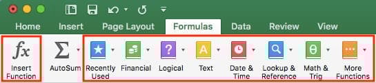
The more you use various formulas in Excel, the easier it’ll be to remember them and perform them manually. Nonetheless, the suite of icons above is a handy catalog of formulas you can browse and refer back to as you hone your spreadsheet skills.

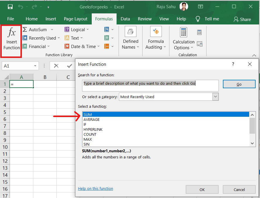
Excel formulas are also called «functions.» To insert one into your spreadsheet, highlight a cell in which you want to run a formula, then click the far-left icon, «Insert Function,» to browse popular formulas and what they do. That browsing window will look like this:

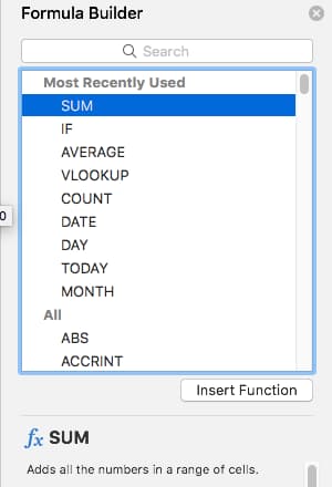Want a more sorted browsing experience? Use any of the icons we’ve highlighted (inside the long red rectangle in the first screenshot above) to find formulas related to a variety of common subjects — such as finance, logic, and more. Once you’ve found the formula that suits your needs, click «Insert Function,» as shown in the window above.

Now, let’s do a deeper dive into some of the most crucial Excel formulas and how to perform each one in typical situations.

To help you use Excel more effectively (and save a ton of time), we’ve compiled a list of essential formulas, keyboard shortcuts, and other small tricks and functions you should know.

NOTE: The following formulas apply to the latest version of Excel. If you’re using a slightly older version of Excel, the location of each feature mentioned below might be slightly different.

1. SUM  

All Excel formulas begin with the equals sign, =, followed by a specific text tag denoting the formula you’d like Excel to perform. 

The SUM formula in Excel is one of the most basic formulas you can enter into a spreadsheet, allowing you to find the sum (or total) of two or more values. To perform the SUM formula, enter the values you’d like to add together using the format, =SUM(value 1, value 2, etc).

The values you enter into the SUM formula can either be actual numbers or equal to the number in a specific cell of your spreadsheet. 

• To find the SUM of 30 and 80, for example, type the following formula into a cell of your spreadsheet: =SUM(30, 80). Press «Enter,» and the cell will produce the total of both numbers: 110. 
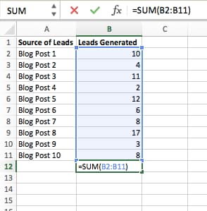
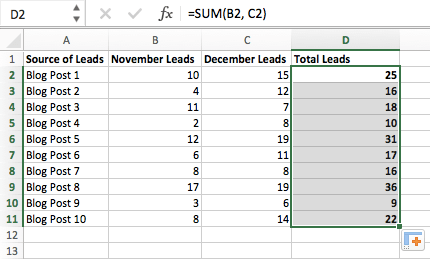
• To find the SUM of the values in cells B2 and B11, for example, type the following formula into a cell of your spreadsheet: =SUM(B2, B11). Press «Enter,» and the cell will produce the total of the numbers currently filled in cells B2 and B11. If there are no numbers in either cell, the formula will return 0. 

Keep in mind you can also find the total value of a list of numbers in Excel. To find the SUM of the values in cells B2 through B11, type the following formula into a cell of your spreadsheet: =SUM(B2:B11). Note the colon between both cells, rather than a comma. See how this might look in an Excel spreadsheet for a content marketer, below:

2. IF

The IF formula in Excel is denoted =IF(logical_test, value_if_true, value_if_false). This allows you to enter a text value into the cell «if» something else in your spreadsheet is true or false. For example, =IF(D2=»Gryffindor»,»10″,»0″) would award 10 points to cell D2 if that cell contained the word «Gryffindor.»

There are times when we want to know how many times a value appears in our spreadsheets. But there are also those times when we want to find the cells that contain those values, and input specific data next to it.

We’ll go back to Sprung’s example for this one. If we want to award 10 points to everyone who belongs in the Gryffindor house, instead of manually typing in 10’s next to each Gryffindor student’s name, we’ll use the IF-THEN formula to say: If the student is in Gryffindor, then he or she should get ten points.

• The formula: IF(logical_test, value_if_true, value_if_false)
  • Logical_Test: The logical test is the «IF» part of the statement. In this case, the logic is D2=»Gryffindor.» Make sure your Logical_Test value is in quotation marks.
  • Value_if_True: If the value is true — that is, if the student lives in Gryffindor — this value is the one that we want to be displayed. In this case, we want it to be the number 10, to indicate that the student was awarded the 10 points. Note: Only use quotation marks if you want the result to be text instead of a number.
  • Value_if_False: If the value is false — and the student does not live in Gryffindor — we want the cell to show «0,» for 0 points.
• Formula in below example: =IF(D2=»Gryffindor»,»10″,»0″)

3. Percentage

To perform the percentage formula in Excel, enter the cells you’re finding a percentage for in the format, =A1/B1. To convert the resulting decimal value to a percentage, highlight the cell, click the Home tab, and select «Percentage» from the numbers dropdown.

There isn’t an Excel «formula» for percentages per se, but Excel makes it easy to convert the value of any cell into a percentage so you’re not stuck calculating and reentering the numbers yourself.

The basic setting to convert a cell’s value into a percentage is under Excel’s Home tab. Select this tab, highlight the cell(s) you’d like to convert to a percentage, and click into the dropdown menu next to Conditional Formatting (this menu button might say «General» at first). Then, select «Percentage» from the list of options that appears. This will convert the value of each cell you’ve highlighted into a percentage. See this feature below.

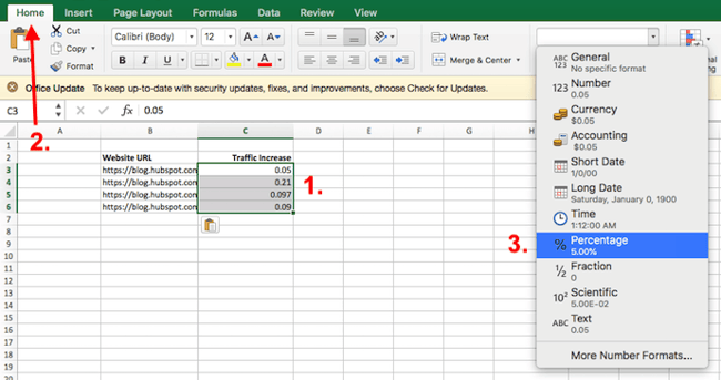
Keep in mind if you’re using other formulas, such as the division formula (denoted =A1/B1), to return new values, your values might show up as decimals by default. Simply highlight your cells before or after you perform this formula, and set these cells’ format to «Percentage» from the Home tab — as shown above.

4. Subtraction

To perform the subtraction formula in Excel, enter the cells you’re subtracting in the format, =SUM(A1, -B1). This will subtract a cell using the SUM formula by adding a negative sign before the cell you’re subtracting. For example, if A1 was 10 and B1 was 6, =SUM(A1, -B1) would perform 10 + -6, returning a value of 4.

Like percentages, subtracting doesn’t have its own formula in Excel either, but that doesn’t mean it can’t be done. You can subtract any values (or those values inside cells) two different ways.

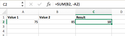
• Using the =SUM formula. To subtract multiple values from one another, enter the cells you’d like to subtract in the format =SUM(A1, -B1), with a negative sign (denoted with a hyphen) before the cell whose value you’re subtracting. Press enter to return the difference between both cells included in the parentheses. See how this looks in the screenshot above.
• Using the format, =A1-B1. To subtract multiple values from one another, simply type an equals sign followed by your first value or cell, a hyphen, and the value or cell you’re subtracting. Press Enter to return the difference between both values.

5. Multiplication

To perform the multiplication formula in Excel, enter the cells you’re multiplying in the format, =A1*B1. This formula uses an asterisk to multiply cell A1 by cell B1. For example, if A1 was 10 and B1 was 6, =A1*B1 would return a value of 60.

You might think multiplying values in Excel has its own formula or uses the «x» character to denote multiplication between multiple values. Actually, it’s as easy as an asterisk — *.

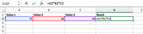
To multiply two or more values in an Excel spreadsheet, highlight an empty cell. Then, enter the values or cells you want to multiply together in the format, =A1*B1*C1 … etc. The asterisk will effectively multiply each value included in the formula.

Press Enter to return your desired product. See how this looks in the screenshot above.

6. Division

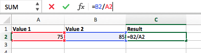
To perform the division formula in Excel, enter the cells you’re dividing in the format, =A1/B1. This formula uses a forward slash, «/,» to divide cell A1 by cell B1. For example, if A1 was 5 and B1 was 10, =A1/B1 would return a decimal value of 0.5.

Division in Excel is one of the simplest functions you can perform. To do so, highlight an empty cell, enter an equals sign, «=,» and follow it up with the two (or more) values you’d like to divide with a forward slash, «/,» in between. The result should be in the following format: =B2/A2, as shown in the screenshot below.

Hit Enter, and your desired quotient should appear in the cell you initially highlighted.

7. DATE

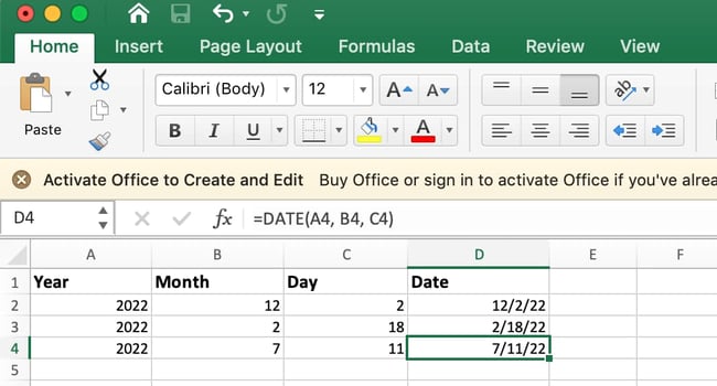
The Excel DATE formula is denoted =DATE(year, month, day). This formula will return a date that corresponds to the values entered in the parentheses — even values referred from other cells. For example, if A1 was 2018, B1 was 7, and C1 was 11, =DATE(A1,B1,C1) would return 7/11/2018.

Creating dates in the cells of an Excel spreadsheet can be a fickle task every now and then. Luckily, there’s a handy formula to make formatting your dates easy. There are two ways to use this formula:

• Create dates from a series of cell values. To do this, highlight an empty cell, enter «=DATE,» and in parentheses, enter the cells whose values create your desired date — starting with the year, then the month number, then the day. The final format should look like this: =DATE(year, month, day). See how this looks in the screenshot below.
• Automatically set today’s date. To do this, highlight an empty cell and enter the following string of text: =DATE(YEAR(TODAY()), MONTH(TODAY()), DAY(TODAY())). Pressing enter will return the current date you’re working in your Excel spreadsheet.

In either usage of Excel’s date formula, your returned date should be in the form of «mm/dd/yy» — unless your Excel program is formatted differently.

8. Array

An array formula in Excel surrounds a simple formula in brace characters using the format, {=(Start Value 1:End Value 1)*(Start Value 2:End Value 2)}. By pressing ctrl+shift+center, this will calculate and return value from multiple ranges, rather than just individual cells added to or multiplied by one another.

Calculating the sum, product, or quotient of individual cells is easy — just use the =SUM formula and enter the cells, values, or range of cells you want to perform that arithmetic on. But what about multiple ranges? How do you find the combined value of a large group of cells?

Numerical arrays are a useful way to perform more than one formula at the same time in a single cell so you can see one final sum, difference, product, or quotient. If you’re looking to find total sales revenue from several sold units, for example, the array formula in Excel is perfect for you. Here’s how you’d do it:

1. To start using the array formula, type «=SUM,» and in parentheses, enter the first of two (or three, or four) ranges of cells you’d like to multiply together. Here’s what your progress might look like: =SUM(C2:C5
2. Next, add an asterisk after the last cell of the first range you included in your formula. This stands for multiplication. Following this asterisk, enter your second range of cells. You’ll be multiplying this second range of cells by the first. Your progress in this formula should now look like this: =SUM(C2:C5*D2:D5)
3. Ready to press Enter? Not so fast … Because this formula is so complicated, Excel reserves a different keyboard command for arrays. Once you’ve closed the parentheses on your array formula, press Ctrl+Shift+Enter. This will recognize your formula as an array, wrapping your formula in brace characters and successfully returning your product of both ranges combined.

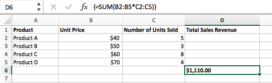
In revenue calculations, this can cut down on your time and effort significantly. See the final formula in the screenshot above.

9. COUNT

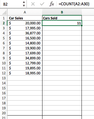
The COUNT formula in Excel is denoted =COUNT(Start Cell:End Cell). This formula will return a value that is equal to the number of entries found within your desired range of cells. For example, if there are eight cells with entered values between A1 and A10, =COUNT(A1:A10) will return a value of 8.

The COUNT formula in Excel is particularly useful for large spreadsheets, wherein you want to see how many cells contain actual entries. Don’t be fooled: This formula won’t do any math on the values of the cells themselves. This formula is simply to find out how many cells in a selected range are occupied with something.

Using the formula in bold above, you can easily run a count of active cells in your spreadsheet. The result will look a little something like this:

10. AVERAGE

To perform the average formula in Excel, enter the values, cells, or range of cells of which you’re calculating the average in the format, =AVERAGE(number1, number2, etc.) or =AVERAGE(Start Value:End Value). This will calculate the average of all the values or range of cells included in the parentheses.

Finding the average of a range of cells in Excel keeps you from having to find individual sums and then performing a separate division equation on your total. Using =AVERAGE as your initial text entry, you can let Excel do all the work for you.

For reference, the average of a group of numbers is equal to the sum of those numbers, divided by the number of items in that group.

11. SUMIF

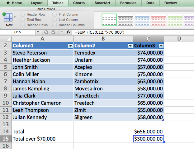
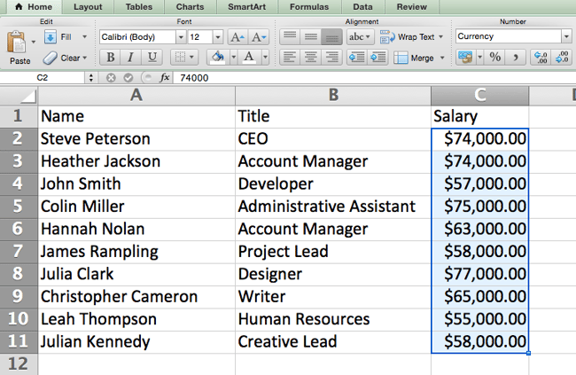
The SUMIF formula in Excel is denoted =SUMIF(range, criteria, [sum range]). This will return the sum of the values within a desired range of cells that all meet one criterion. For example, =SUMIF(C3:C12,»>70,000″) would return the sum of values between cells C3 and C12 from only the cells that are greater than 70,000.

Let’s say you want to determine the profit you generated from a list of leads who are associated with specific area codes, or calculate the sum of certain employees’ salaries — but only if they fall above a particular amount. Doing that manually sounds a bit time-consuming, to say the least.

With the SUMIF function, it doesn’t have to be — you can easily add up the sum of cells that meet certain criteria, like in the salary example above.

• The formula: =SUMIF(range, criteria, [sum_range])
  • Range: The range that is being tested using your criteria.
  • Criteria: The criteria that determine which cells in Criteria_range1 will be added together
  • [Sum_range]: An optional range of cells you’re going to add up in addition to the first Range entered. This field may be omitted.

In the example below, we wanted to calculate the sum of the salaries that were greater than $70,000. The SUMIF function added up the dollar amounts that exceeded that number in the cells C3 through C12, with the formula =SUMIF(C3:C12,»>70,000″).

12. TRIM

The TRIM formula in Excel is denoted =TRIM(text). This formula will remove any spaces entered before and after the text entered in the cell. For example, if A2 includes the name » Steve Peterson» with unwanted spaces before the first name, =TRIM(A2) would return «Steve Peterson» with no spaces in a new cell.

Email and file sharing are wonderful tools in today’s workplace. That is, until one of your colleagues sends you a worksheet with some really funky spacing. Not only can those rogue spaces make it difficult to search for data, but they also affect the results when you try to add up columns of numbers.

Rather than painstakingly removing and adding spaces as needed, you can clean up any irregular spacing using the TRIM function, which is used to remove extra spaces from data (except for single spaces between words).

• The formula: =TRIM(text).
  • Text: The text or cell from which you want to remove spaces.

Here’s an example of how we used the TRIM function to remove extra spaces before a list of names. To do so, we entered =TRIM(«A2») into the Formula Bar, and replicated this for each name below it in a new column next to the column with unwanted spaces.

Below are some other Excel formulas you might find useful as your data management needs grow.

13. LEFT, MID, and RIGHT

Let’s say you have a line of text within a cell that you want to break down into a few different segments. Rather than manually retyping each piece of the code into its respective column, users can leverage a series of string functions to deconstruct the sequence as needed: LEFT, MID, or RIGHT.

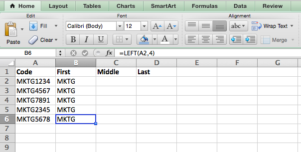
LEFT

• Purpose: Used to extract the first X numbers or characters in a cell.
• The formula: =LEFT(text, number_of_characters)
  • Text: The string that you wish to extract from.
  • Number_of_characters: The number of characters that you wish to extract starting from the left-most character.

In the example below, we entered =LEFT(A2,4) into cell B2, and copied it into B3:B6. That allowed us to extract the first 4 characters of the code.

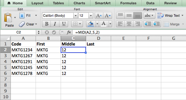
MID

• Purpose: Used to extract characters or numbers in the middle based on position.
• The formula: =MID(text, start_position, number_of_characters)
  • Text: The string that you wish to extract from.
  • Start_position: The position in the string that you want to begin extracting from. For example, the first position in the string is 1.
  • Number_of_characters: The number of characters that you wish to extract.

In this example, we entered =MID(A2,5,2) into cell B2, and copied it into B3:B6. That allowed us to extract the two numbers starting in the fifth position of the code.

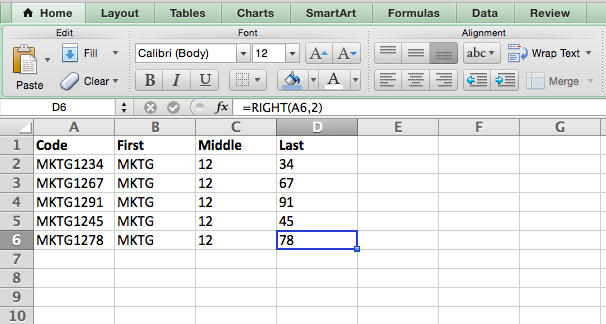
RIGHT

• Purpose: Used to extract the last X numbers or characters in a cell.
• The formula: =RIGHT(text, number_of_characters)
  • Text: The string that you wish to extract from.
  • Number_of_characters: The number of characters that you want to extract starting from the right-most character.

For the sake of this example, we entered =RIGHT(A2,2) into cell B2, and copied it into B3:B6. That allowed us to extract the last two numbers of the code.

14. VLOOKUP

This one is an oldie, but a goodie — and it’s a bit more in depth than some of the other formulas we’ve listed here. But it’s especially helpful for those times when you have two sets of data on two different spreadsheets, and want to combine them into a single spreadsheet.

My colleague, Rachel Sprung — whose «How to Use Excel» tutorial is a must-read for anyone who wants to learn — uses a list of names, email addresses, and companies as an example. If you have a list of people’s names next to their email addresses in one spreadsheet, and a list of those same people’s email addresses next to their company names in the other, but you want the names, email addresses, and company names of those people to appear in one place — that’s where VLOOKUP comes in.

Note: When using this formula, you must be certain that at least one column appears identically in both spreadsheets. Scour your data sets to make sure the column of data you’re using to combine your information is exactly the same, including no extra spaces.

• The formula: VLOOKUP(lookup value, table array, column number, [range lookup])
  • Lookup Value: The identical value you have in both spreadsheets. Choose the first value in your first spreadsheet. In Sprung’s example that follows, this means the first email address on the list, or cell 2 (C2).
  • Table Array: The range of columns on Sheet 2 you’re going to pull your data from, including the column of data identical to your lookup value (in our example, email addresses) in Sheet 1 as well as the column of data you’re trying to copy to Sheet 1. In our example, this is «Sheet2!A:B.» «A» means Column A in Sheet 2, which is the column in Sheet 2 where the data identical to our lookup value (email) in Sheet 1 is listed. The «B» means Column B, which contains the information that’s only available in Sheet 2 that you want to translate to Sheet 1.
  • Column Number: The table array tells Excel where (which column) the new data you want to copy to Sheet 1 is located. In our example, this would be the «House» column, the second one in our table array, making it column number 2.
  • Range Lookup: Use FALSE to ensure you pull in only exact value matches.
• The formula with variables from Sprung’s example below: =VLOOKUP(C2,Sheet2!A:B,2,FALSE)

In this example, Sheet 1 and Sheet 2 contain lists describing different information about the same people, and the common thread between the two is their email addresses. Let’s say we want to combine both datasets so that all the house information from Sheet 2 translates over to Sheet 1. Here’s how that would work:

15. RANDOMIZE

There’s a great article that likens Excel’s RANDOMIZE formula to shuffling a deck of cards. The entire deck is a column, and each card — 52 in a deck — is a row. «To shuffle the deck,» writes Steve McDonnell, «you can compute a new column of data, populate each cell in the column with a random number, and sort the workbook based on the random number field.»

In marketing, you might use this feature when you want to assign a random number to a list of contacts — like if you wanted to experiment with a new email campaign and had to use blind criteria to select who would receive it. By assigning numbers to said contacts, you could apply the rule, “Any contact with a figure of 6 or above will be added to the new campaign.”

• The formula: RAND()
  • Start with a single column of contacts. Then, in the column adjacent to it, type “RAND()” — without the quotation marks — starting with the top contact’s row.
• • RANDBETWEEN allows you to dictate the range of numbers that you want to be assigned. In the case of this example, I wanted to use one through 10.
  • bottom: The lowest number in the range.
  • top: The highest number in the range,For the example below: RANDBETWEEN(bottom,top)
  • Formula in below example: =RANDBETWEEN(1,10)

Helpful stuff, right? Now for the icing on the cake: Once you’ve mastered the Excel formula you need, you’ll want to replicate it for other cells without rewriting the formula. And luckily, there’s an Excel function for that, too. Check it out below.

Sometimes, you might want to run the same formula across an entire row or column of your spreadsheet. Let’s say, for example, you have a list of numbers in columns A and B of a spreadsheet and want to enter individual totals of each row into column C.

Obviously, it would be too tedious to adjust the values of the formula for each cell so you’re finding the total of each row’s respective numbers. Luckily, Excel allows you to automatically complete the column; all you have to do is enter the formula in the first row. Check out the following steps: 

1. Type your formula into an empty cell and press «Enter» to run the formula.
2. Hover your cursor over the bottom-right corner of the cell containing the formula. You’ll see a small, bold «+» symbol appear.
3. While you can double-click this symbol to automatically fill the entire column with your formula, you can also click and drag your cursor down manually to fill only a specific length of the column.Once you’ve reached the last cell in the column you’d like to enter your formula, release your mouse to copy the formula. Then, simply check each new value to ensure it corresponds to the correct cells.

Excel Keyboard Shortcuts

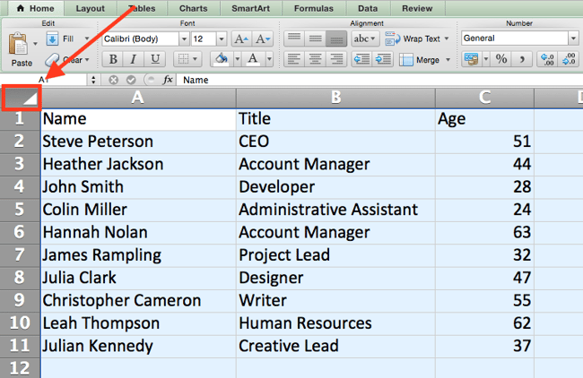
1. Quickly select rows, columns, or the whole spreadsheet.

Perhaps you’re crunched for time. I mean, who isn’t? No time, no problem. You can select your entire spreadsheet in just one click. All you have to do is simply click the tab in the top-left corner of your sheet to highlight everything all at once.

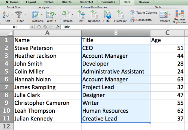
Just want to select everything in a particular column or row? That’s just as easy with these shortcuts:

For Mac:

• Select Column = Command + Shift + Down/Up
• Select Row = Command + Shift + Right/Left

For PC:

• Select Column = Control + Shift + Down/Up
• Select Row = Control + Shift + Right/Left

This shortcut is especially helpful when you’re working with larger data sets, but only need to select a specific piece of it.

2. Quickly open, close, or create a workbook.

Need to open, close, or create a workbook on the fly? The following keyboard shortcuts will enable you to complete any of the above actions in less than a minute’s time.

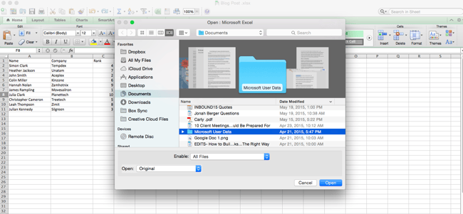
For Mac:

• Open = Command + O
• Close = Command + W
• Create New = Command + N

For PC:

• Open = Control + O
• Close = Control + F4
• Create New = Control + N

3. Format numbers into currency.

Have raw data that you want to turn into currency? Whether it be salary figures, marketing budgets, or ticket sales for an event, the solution is simple. Just highlight the cells you wish to reformat, and select Control + Shift + $.

The numbers will automatically translate into dollar amounts — complete with dollar signs, commas, and decimal points.

Note: This shortcut also works with percentages. If you want to label a column of numerical values as «percent» figures, replace «$» with «%».

4. Insert current date and time into a cell.

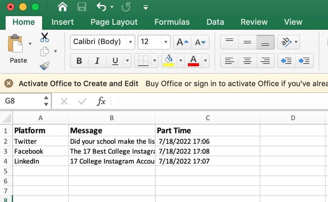
Whether you’re logging social media posts, or keeping track of tasks you’re checking off your to-do list, you might want to add a date and time stamp to your worksheet. Start by selecting the cell to which you want to add this information.

Then, depending on what you want to insert, do one of the following:

• Insert current date = Control + ; (semi-colon)
• Insert current time = Control + Shift + ; (semi-colon)
• Insert current date and time = Control + ; (semi-colon), SPACE, and then Control + Shift + ; (semi-colon).

Other Excel Tricks

1. Customize the color of your tabs.

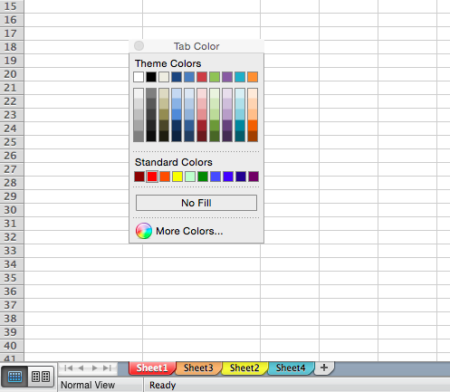
If you’ve got a ton of different sheets in one workbook — which happens to the best of us — make it easier to identify where you need to go by color-coding the tabs. For example, you might label last month’s marketing reports with red, and this month’s with orange.

Simply right click a tab and select «Tab Color.» A popup will appear that allows you to choose a color from an existing theme, or customize one to meet your needs.

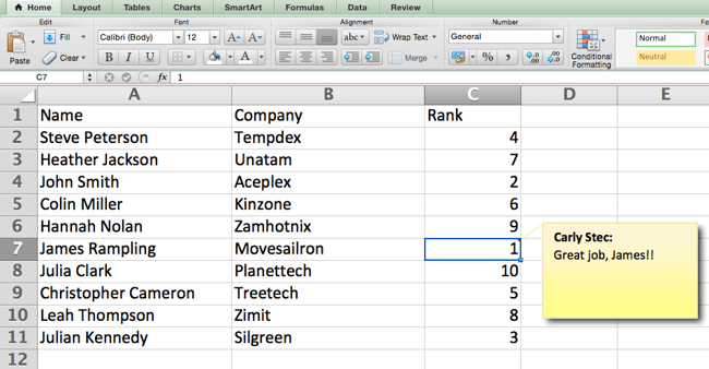
2. Add a comment to a cell.

When you want to make a note or add a comment to a specific cell within a worksheet, simply right-click the cell you want to comment on, then click Insert Comment. Type your comment into the text box, and click outside the comment box to save it.

Cells that contain comments display a small, red triangle in the corner. To view the comment, hover over it.

3. Copy and duplicate formatting.

If you’ve ever spent some time formatting a sheet to your liking, you probably agree that it’s not exactly the most enjoyable activity. In fact, it’s pretty tedious.

For that reason, it’s likely that you don’t want to repeat the process next time — nor do you have to. Thanks to Excel’s Format Painter, you can easily copy the formatting from one area of a worksheet to another.

Select what you’d like to replicate, then select the Format Painter option — the paintbrush icon — from the dashboard. The pointer will then display a paintbrush, prompting you to select the cell, text, or entire worksheet to which you want to apply that formatting, as shown below:

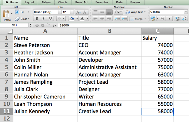
4. Identify duplicate values.

In many instances, duplicate values — like duplicate content when managing SEO — can be troublesome if gone uncorrected. In some cases, though, you simply need to be aware of it.

Whatever the situation may be, it’s easy to surface any existing duplicate values within your worksheet in just a few quick steps. To do so, click into the Conditional Formatting option, and select Highlight Cell Rules > Duplicate Values

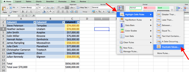
Using the popup, create the desired formatting rule to specify which type of duplicate content you wish to bring forward.

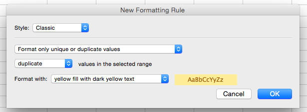
In the example above, we were looking to identify any duplicate salaries within the selected range, and formatted the duplicate cells in yellow.

5. Correcting a ### value error.

If the column isn’t wide enough to display the contents in the cell, Excel may display ### instead. To fix and make the column wider, simply double-click the top right corner of the column header and drag it to the size you want. 

Alternatively, you could also shrink the contents to fit the cell by going: 

 Home > Alignment and then check the Shrink to fit box in the Format Cells dialog box.

Excel Shortcuts Save You Time

In marketing, the use of Excel is pretty inevitable — but with these tricks, it doesn’t have to be so daunting. As they say, practice makes perfect. The more you use these formulas, shortcuts, and tricks, the more they’ll become second nature.

Editor’s note: This post was originally published in January 2019 and has been updated for comprehensiveness.

Excel formulas allow you to identify relationships between values in your spreadsheet’s cells, perform mathematical calculations with those values, and return the resulting value in the cell of your choice. Sum, subtraction, percentage, division, average, and even dates/times are among the formulas that can be performed automatically. For example, =A1+A2+A3+A4+A5, which finds the sum of the range of values from cell A1 to cell A5.

Excel Functions: A formula is a mathematical expression that computes the value of a cell. Functions are predefined formulas that are already in Excel. Functions carry out specific calculations in a specific order based on the values specified as arguments or parameters. For example, =SUM (A1:A10). This function adds up all the values in cells A1 through A10.

How to Insert Formulas in Excel?

This horizontal menu, shown below, in more recent versions of Excel allows you to find and insert Excel formulas into specific cells of your spreadsheet. On the Formulas tab, you can find all available Excel functions in the Function Library:

The more you use Excel formulas, the easier it will be to remember and perform them manually. Excel has over 400 functions, and the number is increasing from version to version. The formulas can be inserted into Excel using the following method:

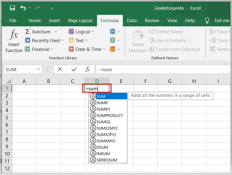
1. Simple insertion of the formula(Typing a formula in the cell):

Typing a formula into a cell or the formula bar is the simplest way to insert basic Excel formulas. Typically, the process begins with typing an equal sign followed by the name of an Excel function. Excel is quite intelligent in that it displays a pop-up function hint when you begin typing the name of the function.

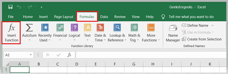
2. Using the Insert Function option on the Formulas Tab:

If you want complete control over your function insertion, use the Excel Insert Function dialogue box. To do so, go to the Formulas tab and select the first menu, Insert Function. All the functions will be available in the dialogue box.

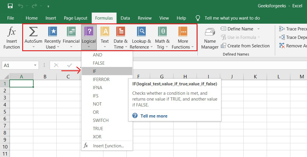
3. Choosing a Formula from One of the Formula Groups in the Formula Tab:

This option is for those who want to quickly dive into their favorite functions. Navigate to the Formulas tab and select your preferred group to access this menu. Click to reveal a sub-menu containing a list of functions. You can then choose your preference. If your preferred group isn’t on the tab, click the More Functions option — it’s most likely hidden there.

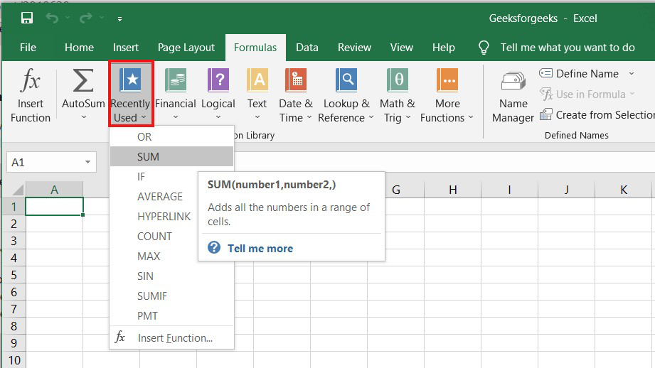
4. Use Recently Used Tabs for Quick Insertion:

If retyping your most recent formula becomes tedious, use the Recently Used menu. It’s on the Formulas tab, the third menu option after AutoSum.

Basic Excel Formulas and Functions:

1. SUM:

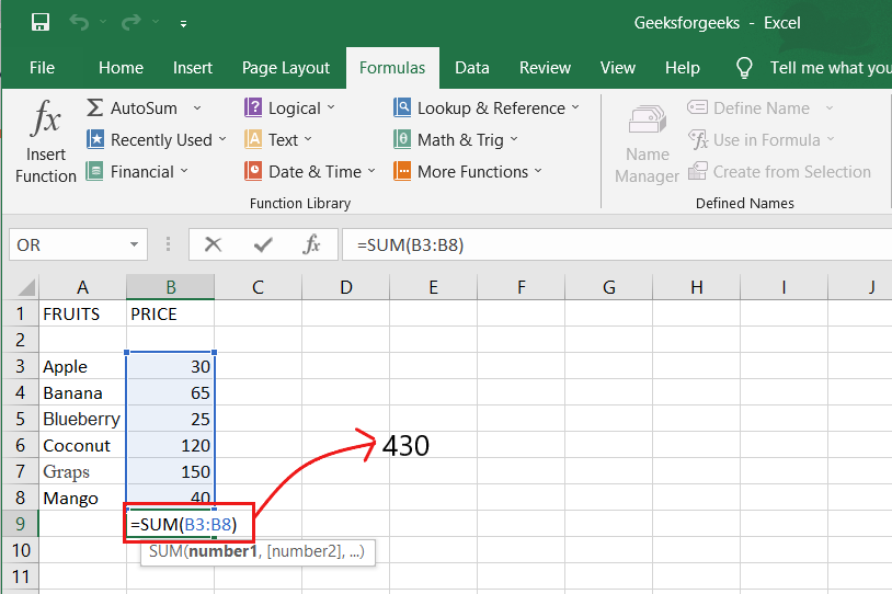
The SUM formula in Excel is one of the most fundamental formulas you can use in a spreadsheet, allowing you to calculate the sum (or total) of two or more values. To use the SUM formula, enter the values you want to add together in the following format: =SUM(value 1, value 2,…..).

Example: In the below example to calculate the sum of price of all the fruits, in B9 cell type =SUM(B3:B8). this will calculate the sum of B3, B4, B5, B6, B7, B8 Press “Enter,” and the cell will produce the sum: 430. 

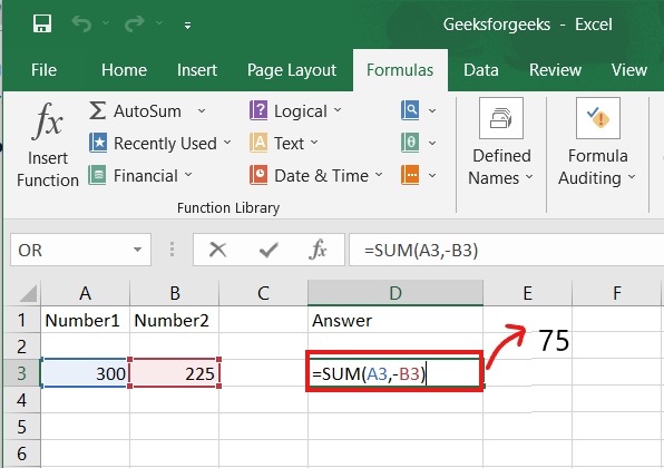
2. SUBTRACTION:

To use the subtraction formula in Excel, enter the cells you want to subtract in the format =SUM (A1, -B1). This will subtract a cell from the SUM formula by appending a negative sign before the cell being subtracted.

For example, if A3 was 300 and B3 was 225, =SUM(A1, -B1) would perform 300 + -225, returning a value of 75 in D3 cell.

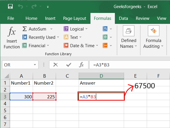
3. MULTIPLICATION:

In Excel, enter the cells to be multiplied in the format =A3*B3 to perform the multiplication formula. An asterisk is used in this formula to multiply cell A3 by cell B3.

For example, if A3 was 300 and B3 was 225, =A1*B1 would return a value of 67500.

Highlight an empty cell in an Excel spreadsheet to multiply two or more values. Then, in the format =A1*B1…, enter the values or cells you want to multiply together. The asterisk effectively multiplies each value in the formula.

To return your desired product, press Enter. Take a look at the screenshot above to see how this looks.

4. DIVISION:

To use the division formula in Excel, enter the dividing cells in the format =A3/B3. This formula divides cell A3 by cell B3 with a forward slash, “/.”

For example, if A3 was 300 and B3 was 225, =A3/B3 would return a decimal value of 1.333333333.

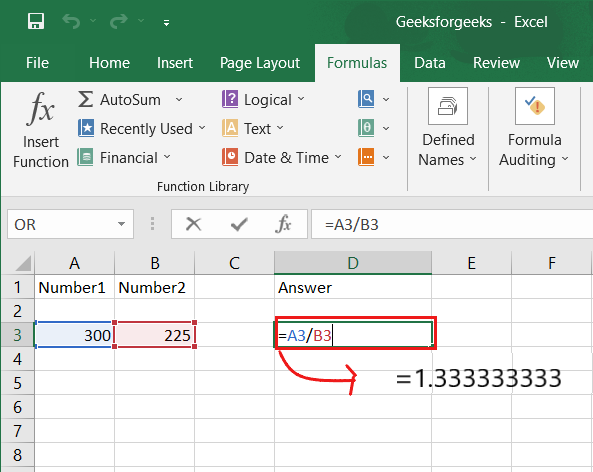
Division in Excel is one of the most basic functions available. To do so, highlight an empty cell, enter an equals sign, “=,” and then the two (or more) values you want to divide, separated by a forward slash, “/.” The output should look like this: =A3/B3, as shown in the screenshot above.

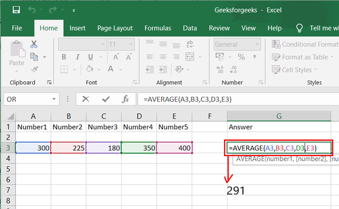
5. AVERAGE:

The AVERAGE function finds an average or arithmetic mean of numbers. to find the average of the numbers type = AVERAGE(A3.B3,C3….) and press ‘Enter’ it will produce average of the numbers in the cell.

For example, if A3 was 300, B3 was 225, C3 was 180, D3 was 350, E3 is 400 then =AVERAGE(A3,B3,C3,D3,E3) will produce 291.

6. IF formula:

In Excel, the IF formula is denoted as =IF(logical test, value if true, value if false). This lets you enter a text value into a cell “if” something else in your spreadsheet is true or false.

For example, You may need to know which values in column A are greater than three. Using the =IF formula, you can quickly have Excel auto-populate a “yes” for each cell with a value greater than 3 and a “no” for each cell with a value less than 3.

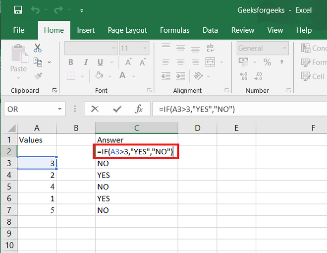
7. PERCENTAGE:

To use the percentage formula in Excel, enter the cells you want to calculate the percentage for in the format =A1/B1. To convert the decimal value to a percentage, select the cell, click the Home tab, and then select “Percentage” from the numbers dropdown.

There isn’t a specific Excel “formula” for percentages, but Excel makes it simple to convert the value of any cell into a percentage so you don’t have to calculate and reenter the numbers yourself.

The basic setting for converting a cell’s value to a percentage is found on the Home tab of Excel. Select this tab, highlight the cell(s) you want to convert to a percentage, and then select Conditional Formatting from the dropdown menu (this menu button might say “General” at first). Then, from the list of options that appears, choose “Percentage.” This will convert the value of each highlighted cell into a percentage. This feature can be found further down.

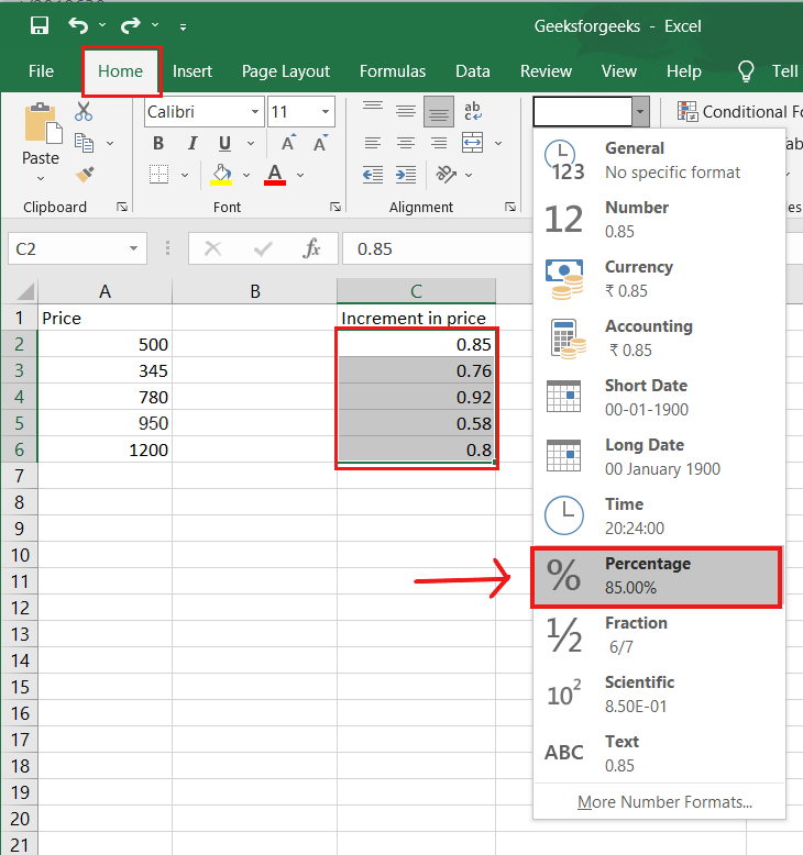
8. CONCATENATE:

CONCATENATE is a useful formula that combines values from multiple cells into the same cell.

For example , =CONCATENATE(A3,B3) will combine Red and Apple to produce RedApple. 

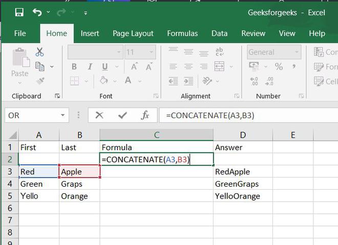
9. DATE:

DATE is the Excel DATE formula =DATE(year, month, day). This formula will return a date corresponding to the values entered in the parentheses, including values referred to from other cells.. For example, if A2 was 2019, B2 was 8, and C1 was 15, =DATE(A1,B1,C1) would return 15-08-2019.

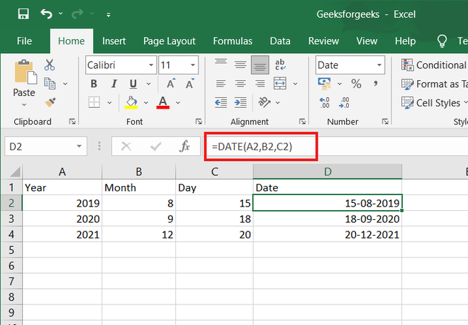
10. TRIM:

The TRIM formula in Excel is denoted =TRIM(text). This formula will remove any spaces that have been entered before and after the text in the cell. For example, if A2 includes the name ” Virat Kohli” with unwanted spaces before the first name, =TRIM(A2) would return “Virat Kohli” with no spaces in a new cell.

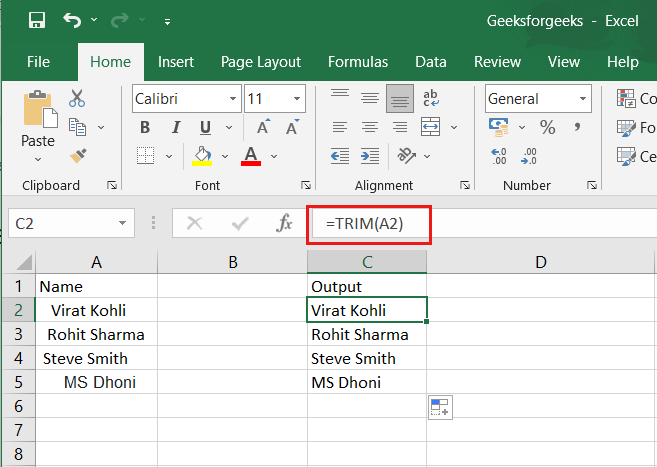
11. LEN:

LEN is the function to count the number of characters in a specific cell when you want to know the number of characters in that cell. =LEN(text) is the formula for this. Please keep in mind that the LEN function in Excel counts all characters, including spaces:

For example,=LEN(A2), returns the total length of the character in cell A2 including spaces.

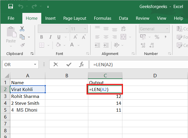
It’s hard to get excited about learning math. It’s something that most of us spend our lives avoiding. It’s also one of the best reasons to use Microsoft Excel for perfect calculations, every time.

Don’t think of these Excel formulas as math for math’s sake. Instead, imagine how these formulas can help you automate your life and skip the trouble of making manual calculations. At the end of this tutorial, you’ll have the skills you need to do all of the following, for example:

• Calculate the average score of your exams.
• Quickly subtotal the invoices you’ve issued to clients.
• Use basic statistics to review a set of data for trends and indicators.

You don’t have to be an accountant to master math in Excel, however. To follow along with this tutorial, make sure to download the example Excel workbook here or click on the blue Download Attachment button on the right side of this tutorial—in either case it’s free to use. 

The Excel workbook has comments and instructions for how to use these formulas. As you follow along in this tutorial, I’ll teach you some of the essential «math» skills. Let’s get started.

Basic Excel Math Formulas Video (Watch and Learn)

If learning from a screencast video is your style, check out the video below to walk through the tutorial. Otherwise, keep reading for a detailed description of how to work with each Excel math formula.

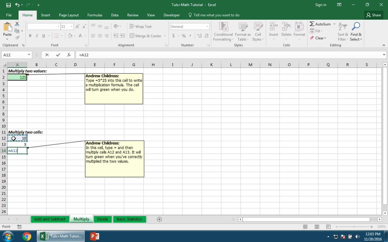
Formula Basics

Before we get started, let’s look at how to use any formula in Microsoft Excel. Whether you’re working with the math formulas in this tutorial or any others, these tips will help you master Excel.

1. Each Formula in Excel Starts with «=»

To type a formula, click in any cell in Microsoft Excel and type the equals sign on your keyboard. This starts a formula.

After the equals sign, you can put an incredible variety of things into the cell. Try typing =4+4 as your very first formula, and press enter to return the result. Excel will output 8, but the formula is still behind the scenes in the spreadsheet.

2. Formulas are Shown in Excel’s Formula Bar

When you’re typing a formula into a cell, you can see the results of the cell once you press enter. But when you select a cell, you can see the formula for that cell in the formula bar.

To use the example from above, the cell will show «8» , but when we click on that cell, the formula bar will show that the cell is adding 4 and 4.

3. How to Build a Formula

In the example above, we typed a simple addition formula to add two numbers. But, you don’t have to type numbers, you can also reference other cells. 

Excel is a grid of cells, with the columns running left to right, each assigned a letter, while the rows are numbered. Each cell is an intersection of a row and a column. The cell where column A and row 3 intersect is called A3, for example.

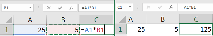
Let’s say that I have two cells with simple numbers, like 1 and 2, and they are in cells A2 and A3. When I type a formula, I can start the formula with «=» as always. Then, I can type:

=A2+A3

…to add those two numbers together. It’s very common to have a sheet with values, and then a separate sheet where calculations are performed. Keep all of these tips in mind while working with this tutorial. For each of the formulas, you can reference cells, or directly type numerical values into the formula. 

If you need to change a formula that you’ve already typed, double click on the cell. You’ll be able to adjust the values in the formula.

Arithmetic in Excel

Now we’ll cover Excel math formulas and walk through how to use them. Let’s start off by exploring the basic arithmetic formula. These are the foundation of math operations.

1. Add and Subtract

Addition and subtraction are two essential math formulas in Excel. Whether you’re adding up your list of business expenses for the month or balancing your checkbook digitally, the addition and subtraction operators are incredibly useful.

Use the tab titled «Add and Subtract» in the workbook for practice.

Add Values

Example:

=24+48

or, reference values in cells with:

=A2+A3

Tip: try adding five or six values to see what happens. Separate each item with a plus sign.

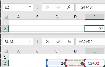
Subtract Values

Example:

=75-25-10

or, reference values in cells with:

=A3-A2

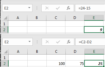
2. Multiplication

To multiply values, use the * operator. Use multiplication instead of adding the same item over and over.

Use the tab titled «Multiply» in the workbook for practice.

Example:

=5*4

or, reference values in cells with:

=A2*A3

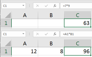
3. Division

Division is helpful when splitting items into groups, for example. Use the «/» operator to divide numbers or the values in cells in your spreadsheet.

Use the tab titled «Divide» in the workbook for practice.

Example:

=20/10

or, reference values in cells with:

=A5/B2

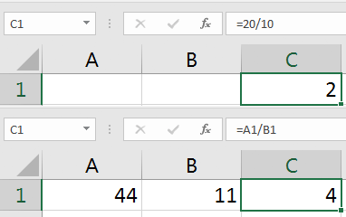
Basic Statistics

Use the tab titled «Basic Statistics» in the workbook for practice.

Now that you know the basic math operators, let’s move onto something more advanced. Basic statistics are helpful to review a set of data and to make informed judgments about it. Let’s cover several popular, simple statistic formulas.

1. Average

To use an average formula in Excel, open your formula with =AVERAGE( and then input your values. Separate each number with a comma. When you press enter, Excel will calculate and output the average.

=AVERAGE(1,3,5,7,10)

The best way to calculate an average is to input your values into separate cells in a single column.

=AVERAGE(A2:A5)

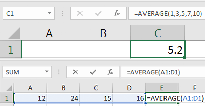
2. Median

The median of a data set is the value that’s in the middle. If you took the numerical values and ordered them from smallest to largest, the median would be smack dab in the middle of that list.

=MEDIAN(1,3,5,7,10)

I’d recommend typing your values into a list of cells, and then using the median formula over a list of cells with values typed in them.

=MEDIAN(A2:A5)

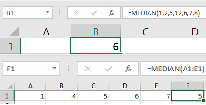
3. Min

If you have a set of data and want to keep your eye on the smallest value, the MIN formula in Excel is useful. You can use the MIN formula with a list of numbers, separated by commas, to find the lowest value in a set. This is very useful when working with large datasets.

=MIN(1,3,5,7,9)

You might want to find the minimum value in a list of data, which is totally possible with a formula such as:

=MIN(A1:E1)

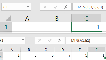
4. Max

The MAX formula in Excel is the polar opposite of MIN; it tells you which value in a set is the largest. You can use it with a list of numbers, separated by commas:

=MAX(1,3,5,7,9)

Or, you can select a list of values in cells, and have Excel return the largest in the set, with a formula like this:

=MAX(A1:E1)

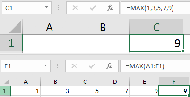
Recap and Keep Learning

I hope this Excel math formulas tutorial helped you think more about what Excel can do for you. With enough practice, your Excel skills will soon seem more natural than grabbing a calculator or doing math on paper. Spreadsheets capture data, and formulas help us understand or modify that data. The operations can be basic, but are at the foundation of important spreadsheets in every company.

It’s always a great idea to use one tutorial to launch more learning. Here are some suggestions

• For more advanced math in equation-like formats, Microsoft’s official documentation has a page titled «Insert or edit an equation or expression.»
• Tuts+ instructor Bob Flisser has a nice tutorial on calculating percentages in Excel.

What are some other math skills that you use in Excel? Leave a reply in the comments if you know a great formula that I don’t.