
Excel for Microsoft 365 Excel for the web Excel 2021 Excel 2019 Excel 2016 Excel 2013 Excel 2010 Excel 2007 More…Less
Let’s say you want to round a number to the nearest whole number because decimal values are not significant to you. Or, you want to round a number to multiples of 10 to simplify an approximation of amounts. There are several ways to round a number.
Change the number of decimal places displayed without changing the number
On a worksheet
-
Select the cells that you want to format.
-
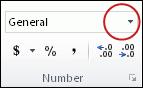
To display more or fewer digits after the decimal point, on the Home tab, in the Number group, click Increase Decimal
 or Decrease Decimal .
 or Decrease Decimal
  .
.In a built-in number format
-
On the Home tab, in the Number group, click the arrow next to the list of number formats, and then click More Number Formats.
-
In the Category list, depending on the data type of your numbers, click Currency, Accounting, Percentage, or Scientific.
-
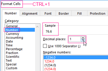
In the Decimal places box, enter the number of decimal places that you want to display.
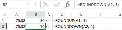
Round a number up
Use the ROUNDUP function. In some cases, you may want to use the EVEN and the ODD functions to round up to the nearest even or odd number.
Round a number down
Use the ROUNDDOWNfunction.
Round a number to the nearest number
Use the ROUND function.
Round a number to a near fraction
Use the ROUND function.
Round a number to a significant digit
Significant digits are digits that contribute to the accuracy of a number.
The examples in this section use the ROUND, ROUNDUP, and ROUNDDOWN functions. They cover rounding methods for positive, negative, whole, and fractional numbers, but the examples shown represent only a very small list of possible scenarios.
The following list contains some general rules to keep in mind when you round numbers to significant digits. You can experiment with the rounding functions and substitute your own numbers and parameters to return the number of significant digits that you want.
-
When rounding a negative number, that number is first converted to its absolute value (its value without the negative sign). The rounding operation then occurs, and then the negative sign is reapplied. Although this may seem to defy logic, it is the way rounding works. For example, using the ROUNDDOWN function to round -889 to two significant digits results in -880. First, -889 is converted to its absolute value of 889. Next, it is rounded down to two significant digits results (880). Finally, the negative sign is reapplied, for a result of -880.
-
Using the ROUNDDOWN function on a positive number always rounds a number down, and ROUNDUP always rounds a number up.
-
The ROUND function rounds a number containing a fraction as follows: If the fractional part is 0.5 or greater, the number is rounded up. If the fractional part is less than 0.5, the number is rounded down.
-
The ROUND function rounds a whole number up or down by following a similar rule to that for fractional numbers; substituting multiples of 5 for 0.5.
-
As a general rule, when you round a number that has no fractional part (a whole number), you subtract the length from the number of significant digits to which you want to round. For example, to round 2345678 down to 3 significant digits, you use the ROUNDDOWN function with the parameter -4, as follows: = ROUNDDOWN(2345678,-4). This rounds the number down to 2340000, with the «234» portion as the significant digits.
Round a number to a specified multiple
There may be times when you want to round to a multiple of a number that you specify. For example, suppose your company ships a product in crates of 18 items. You can use the MROUND function to find out how many crates you will need to ship 204 items. In this case, the answer is 12, because 204 divided by 18 is 11.333, and you will need to round up. The 12th crate will contain only 6 items.
There may also be times where you need to round a negative number to a negative multiple or a number that contains decimal places to a multiple that contains decimal places. You can also use the MROUND function in these cases.
Need more help?
Want more options?
Explore subscription benefits, browse training courses, learn how to secure your device, and more.
Communities help you ask and answer questions, give feedback, and hear from experts with rich knowledge.
На чтение 1 мин
Функция ОКРУГЛ (ROUND) используется в Excel для округления числа до заданного количества десятичных разрядов.
Содержание
- Что возвращает функция
- Синтаксис
- Аргументы функции
- Дополнительная информация
- Примеры использования функции ОКРУГЛ в Excel
Что возвращает функция
Число, округленное, до заданного количества десятичных разрядов.
 Больше лайфхаков в нашем Telegram Подписаться
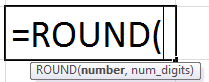
Синтаксис
=ROUND(number, num_digits) — английская версия
=ОКРУГЛ(число;число_разрядов) — русская версия
Аргументы функции
- number (число) — число, которое вы хотите округлить;
- num_digits (число_разрядов) — значение десятичного разряда, до которого вы хотите округлить первый аргумент функции.
Дополнительная информация
- если аргумент num_digits (число_разрядов) больше “0”, то число округляется до указанного количества десятичных знаков. Например, =ROUND(500.51,1) или =ОКРУГЛ(500.51;1) вернет “500.5”;
- если аргумент num_digits (число_разрядов) равен “0”, то число округляется до ближайшего целого числа. Например, =ROUND(500.51,0) или =ОКРУГЛ(500.51;0) вернет “501”;
- если аргумент num_digits (число_разрядов) меньше “0”, то число округляется влево от десятичного значения. Например, =ROUND(500.51,-1) или =ОКРУГЛ(500.51;-1) вернет “501”.
Примеры использования функции ОКРУГЛ в Excel
You can round numbers in Excel in several ways: with helping the format of cells and with the help of functions. These two methods should be distinguished: the first only to display or print output, and the second one — for computations and calculations.
With helping functions you can accurate rounding — up or down to the user-specified discharge. And the values obtained computationally, can be used in other formulas and functions. At the same time the rounding by using the format cells does not give the desired result, and the results of calculations with these values will be erroneous. Because the format of the cells, in fact, the value does not change, the only change it its display method. To quickly and easily understand and to avoid mistakes, there are some examples.
How to round the number by the format of the cell
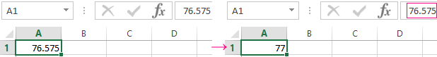
You need to put in the cell A1 the value 76. 575. Clicking with the right mouse button, we called the menu «Format of the cells» to do the same you can through the instrument of «Number» on the main page of the Book. You can also press the hot key combination CTRL+1 for this purpose.
Choose the number format and set decimal places to 0.
The result of rounding:
To assign the number of decimal places we can in the «Accounting» format, «Currency», «Percentage».
Assign the number of decimal places in the «cash» format, «financial», «interest».
As we can see, the rounding occurs according to mathematical laws. The last figure which you need to keep will be increased by one, if it is followed by a figure greater than or equal to «5».
The feature of this option: the more decimal places we leave, the better the result will be got.
How to round a number in Excel
Using the function ROUND (round to user required number of decimal places). To call the «Wizards» we use the fx button. The desired function is in the category of «Mathematical».
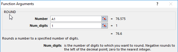
The arguments:
- «Number» — is a reference to a cell with the desired value (A1).
- «Number_digits» — is the value of decimal places to which you want to round (0 – to round to a whole number, 1 – it`ll be left a single decimal place, 2 – is two, etc.).
We are rounding to an integer (not a decimal) now. We use the ROUND function:
- the first argument of the function – is a reference to the cell;
- the second argument is negative «-» (up to tens – is «-1», to hundreds – is «-2», to round a number to thousands – is «-3», etc.).
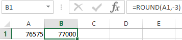
How to round a number in Excel to thousands?
The example rounding of a number to thousands:
The formula: =ROUND(A1,-3)
You can round up not only the number but also the value of the expression.
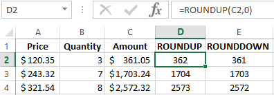
For example, there are findings on price and quantity of good. You need to find a value accurate to ruble (round up to the nearest whole number).
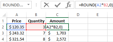
The function’s first argument — is a numeric expression for finding the value.
How to round in large and smaller side in Excel
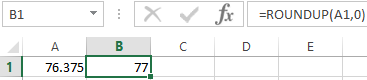
For rounding off in a big way – is the function «ROUNDUP».
The first argument we fill in on the familiar principle – is a reference to a data cell.
The second argument: «0» — round of a decimal to an integer, «1» — the function rounds, leaving one decimal place after the decimal point, etc.
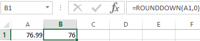
Formula: =ROUNDDOWN(A1,0)
The result:
To round down in Excel, apply the function «ROUNDDOWN».
The example of the formula: =ROUNDDOWN(A1,0).
The result:
The formulas «ROUNDUP» and «ROUNDDOWN» are used for rounding the values of the expressions (product, sum, difference, etc.).
How to round to the nearest whole number in Excel?
To round to the nearest whole in a big way we use the function «ROUNDUP». To round to an integer value in the smaller side we use the function «ROUNDDOWN». The function «ROUND» and format of cells as well allow you to round it to integer, setting the value of digits – is «0» (see above).
In Excel for rounding to the nearest whole number we also apply the function «TRUNC». It just drops the decimal places. In fact, there is no rounding applied. The formula cuts off the numbers to the assigned category.
Compare:
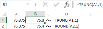
The second argument is «0» — the function cuts off to the nearest whole number; «1» — to the tenth; «2» — to the decimal places, etc.
The special Excel function, which will return only an integer – is «INT». It has the single argument. You can specify a numeric value or a cell reference.
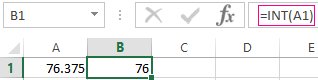
The disadvantage of using function «INT» only rounds down.
Be rounded to an integer in Excel you may using the functions «ROUNDUP» and «ROUNDDOWN». Rounding occurs up or down to the nearest of whole value.
The example of using functions:
The second argument indicates the category to which should be rounded (10 — to tens, 100 — to hundreds, etc.).
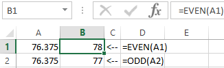
Rounding to the nearest even integer performs the function of «EVEN», to the nearest odd value — is «ODD».
The example of their using:
Why Excel rounds up large numbers?
If cells in a spreadsheet are introduced large numbers (for example, 78568435923100756), the default Excel automatically rounds down them here: 7, 85684 E + 16 – this is a feature of the format cells to «General». To avoid the display of large numbers you need to change the format of the cell with a large number of «Numerical» (the fastest way to press the hot key combination CTRL+SHIFT+1). Then the cell value will display like this: 78 568 435 923 100 756, 00. If you wish, the digit of levels can be reduced: «HOME» — «Decrease Decimal».
In this tutorial, we will learn to round numbers in multiple ways in Microsoft Excel. We can round numbers either via the Home tab or by using different formulas like the ROUND, ROUNDUP, and ROUNDDOWN functions in Excel.
Also read: How to Stop Excel from Rounding?
To directly round numbers without using a formula, here’s what you can do.

- Type a decimal number in a cell with more than 2 or 3 digits after the decimal point.
- Go to the Home tab.
- Under the Number section, select the Increase Decimal or Decrease Decimal icon to round up that number.

You can see that the number has been rounded up after selecting the Decrease Decimal option in Excel.

Using the ROUND function in Excel
The ROUND function is created to round numbers in Excel. Let’s see how we can round numbers with this function.
- Type a decimal number in a cell.
- Type =ROUND( in another blank cell.
- Select the decimal number.
- Put a comma and type the number of digits you want to have after the decimal point.
- Close brackets and press ENTER.


You can see that the ROUND formula has rounded up the number in the cell. Let us try another example by putting 0 digits to be shown.

You can see that the ROUND function has rounded up the two numbers into whole numbers.
Note – Any decimal number that has a number equal to or greater than 0.5 after decimals, then that number gets rounded up to the nearest highest whole number if 0 digits have been applied in the ROUND function.
Using the ROUNDUP function in Excel
The ROUNDUP function is used to round up decimal numbers to the nearest highest decimal point in Excel. Let’s see how we can round up numbers with this function.
- Type a decimal number in a cell.
- Type =ROUNDUP( in another blank cell.
- Select the decimal number.
- Put a comma and type the number of digits you want to have after the decimal point.
- Close brackets and press ENTER.


We can see that the two numbers have been rounded up by the ROUNDUP function in Excel to the nearest highest decimal point.
Let’s now see what results do we get after applying 0 digits to be seen after the decimal point

You can see that both numbers irrespective of any number after the decimal point, get rounded up to the nearest highest whole number by the ROUNDUP function.
You can clearly figure out the difference between the ROUND and the ROUNDUP function when it comes to applying 0 digits in the num_digits argument. The ROUND function will not round up to the nearest whole number until any number equal to greater than 0.5 is entered after the decimal point.
Using the ROUNDDOWN function in Excel
The ROUNDDOWN function, as the name suggests, is contrary to the ROUNDUP function in Excel. It is used to round down decimal numbers to the nearest lowest decimal point. Let’s see how we can round down numbers with this function.
- Type a decimal number in a cell.
- Type =ROUNDDOWN( in another blank cell.
- Select the decimal number.
- Put a comma and type the number of digits you want to have after the decimal point.
- Close brackets and press ENTER.


You can see that the ROUNDDOWN function has rounded down the two numbers in Excel. There is little to no difference in the numbers except that there are only 2 digits to be seen after the decimal point now.
Let’s see the result after putting 0 digits in the num_digits argument.

You can see that both numbers have been rounded down to the nearest lowest whole number regardless of the number being greater or less than 0.5 after the decimal point.
Conclusion
This was all about the round functions in Excel and a step-by-step guide on using and applying them. Feel free to comment your doubts below regarding rounding numbers in Excel, if you have any! Stay tuned for more informative tutorials like this!
References: Microsoft
The ROUND Excel function is a built-in function in Excel that calculates the round number of a given number with the number of digits to be provided as an argument. This formula takes two arguments: the number itself and the number of digits to which we want the number to be rounded up.
For example, suppose cell D1 contains 22.5863. Then, if we want to round that value to two decimal places, we can use the following formula: =ROUND(D1,2). As a result, this function may provide 22.59.
Table of contents
- ROUND in Excel
- ROUND Formula in Excel
- Usage Notes
- Explanation
- How to Open the ROUND Function in Excel?
- How to Use ROUND Function in Excel with Examples
- Example #1
- Example #2
- Example #3
- Example #4
- Example #5
- Other Rounding Functions in Excel
- Things to Remember
- ROUND Excel Function Video
- Recommended Articles
ROUND Formula in Excel
The ROUND Formula in Excel accepts the following parameters and arguments:
Number – The number which has to be rounded.
Num_Digits – The total number of digits to round the number to.
Return Value: The ROUND function returns a numeric value.
Usage Notes
- The ROUND formula in Excel works by rounding the numbers 1-4 down and 5-9 up.
- You can use the ROUND function in Excel for rounding numbers to a specified level of precision. We can use the ROUND function in Excel for rounding to the right or left of the decimal point.
- If num_digits is greater than 0, the number will be rounded to the specified decimal places to the right of the decimal point. For example, =ROUND (16.55, 1) will round 16.55 to 16.6.
- If num_digits is less than 0, the number will be rounded to the left of the decimal point (to the nearest 10, 100, 1000, and so on). For example, =ROUND (16.55, -1) will round 16.55 to the nearest 10 and return 20 as the return value or result.
- If num_digits = 0, the number will be rounded to the nearest integer (no decimal places). For example, =ROUND (16.55, 0) will round 16.55 to 17.
Explanation
The ROUND in Excel follows the general math rules for rounding the numbers. In this ROUND function, the number to the right of the rounding digit will determine whether the number should be rounded upwards or downwards. The rounding digit is considered the least significant after the number is rounded. It also gets changed, depending on whether the digit following it is less or greater than 5.
- If the digit to the right of the rounding digit is 0,1,2,3, or 4, it will not change the rounding digit, and the number will be rounded down.
- If the rounding digit is followed by 5,6,7,8 or 9, the rounding digit will be increased by one, and the number will be rounded up.
Consider the following table to understand the above theory more deeply. In this ROUND in Excel example, we are taking the number 106.864. The position is cell number A2 in the spreadsheet.
| Formula | Result | Description |
|---|---|---|
| =ROUND (A2,2) | 106.86 | The number in A2 is rounded to 2 decimal places. |
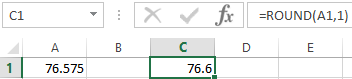
| =ROUND (A2,1) | 106.9 | The number is A2 is rounded to 1 decimal place. |
| =ROUND (A2,0) | 107 | The number in A2 is rounded to the nearest integer. |
| =ROUND (A2,-1) | 110 | The number in A2 is rounded to the nearest multiple of 10. |
| =ROUND (A2-2) | 100 | The number in A2 is rounded to the nearest multiple of 100. |
How to Open the ROUND Function in Excel?
You can download this ROUND Function Excel Template here – ROUND Function Excel Template
- You can insert the desired ROUND formula in the required cell to attain a return value on the argument.
- You can manually open the ROUND formula in the Excel dialog box in the spreadsheet and insert the logical values to attain a return value.
- The spreadsheet below shows the “Formulas” section in the “Menu” bar. Under the “Formulas” section, Click on the “Math & Trig.”
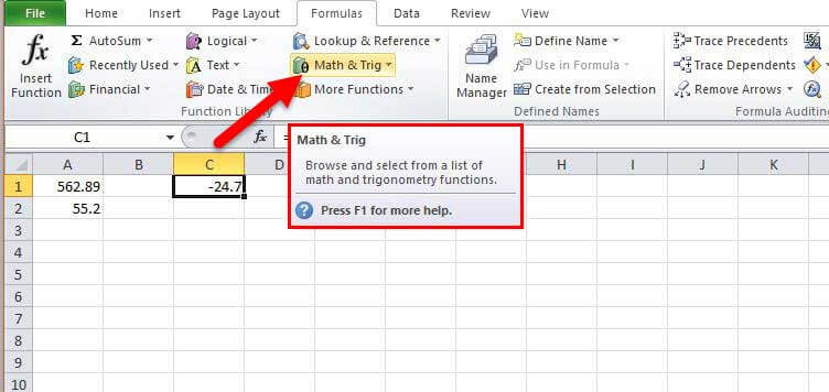
- After clicking the “Math & Trig option,” select “ROUND.” The ROUND formula in the Excel dialog box will open, as shown below.
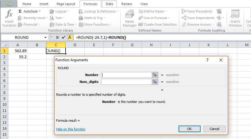
- Now, you can easily put the arguments and attain a return value. Just put the required values on Number and Num_digits. You will get the return value.
How to Use ROUND Function in Excel with Examples
Let us look below at some examples of the ROUND formula in Excel. These examples will help you in exploring the use of the ROUND function.
Based on the above Excel spreadsheet, let’s consider three examples and see the ROUND function return based on the syntax of the function.
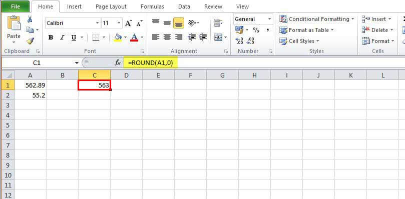
Example #1
When the ROUND formula for Excel written is =ROUND (A1, 0)
Result: 563
You can see the excel spreadsheet below –
Example #2
When the ROUND formula for Excel written is =ROUND (A1, 1)
Result: 562.9
Consider the Excel spreadsheet below-

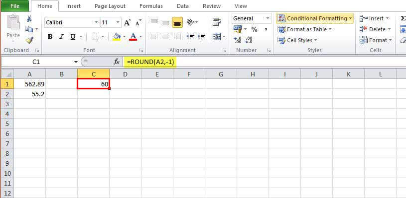
Example #3
When the ROUND formula for Excel written is =ROUND (A2, -1)
Result: 60
Consider the Excel spreadsheet below –
Example #4
When the ROUND formula for Excel is written =ROUND (52.2, -1)
Result: 50
You can consider the excel spreadsheet below –

Example #5
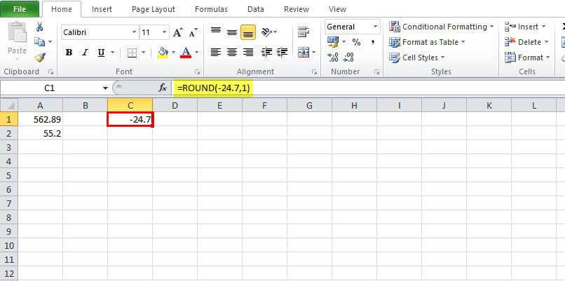
When the ROUND formula for Excel is written =ROUND (-24.57, 1)
Result: -24.7
You can see the excel spreadsheet below –
Other Rounding Functions in Excel
You can also force Excel to always round a number up (away from zero) with the help of the ROUNDUP functionThe ROUNDUP excel function calculates the rounded value of the number to the upward side or the higher side. In other words, it rounds the number away from zero. Being an inbuilt function of Excel, it accepts two arguments–the “number” and the “num_of _digits.” For example, “=ROUNDUP(0.40,1)” returns 0.4.
read more. If you want Excel to always round a number down (towards zero), use the ROUNDDOWN function in Excel. For specifying the multiple (example 0.5) that Excel uses to round, use the MROUND function in excelMROUND is the MATH & TRIGNOMETRY function in Excel, and it is used to round a number to the nearest multiple numbers. For example, =MROUND(50,7), will round the number 50 to 49.read more.
Things to Remember
- The ROUND function returns a number rounded to a specific number of digits.
- The ROUND function is a Math & Trig function.
- The ROUND function works by rounding the numbers 1-4 down and 5-9 up.
- We can round a number up (away from zero) with the help of the ROUNDUP function.
- We can round a number down (towards zero) using the ROUNDDOWN functionROUNDDOWN function is a built-in function in Microsoft Excel. It is used to round off the given number.read more.
ROUND Excel Function Video
Recommended Articles
This article is a guide to ROUND Function in Excel. Here, we discuss the ROUND formula in Excel and how to use the Excel ROUND function, along with Excel examples and downloadable Excel templates. You may also look at these useful functions in Excel: –
- VBA ROUNDUPThe roundup function in VBA decrease the decimal point, and the syntax to use it is: Roundup (Number, Number of Digits After Decimal).read more
- How to use RAND in Excel?The RAND function in Excel, also known as the random function, generates a random value greater than 0 but less than 1, with an even distribution among those numbers when used on multiple cells. read more
- Use INDEX Function in ExcelThe INDEX function in Excel helps extract the value of a cell, which is within a specified array (range) and, at the intersection of the stated row and column numbers.read more
- Concatenate in ExcelThe CONCATENATE function in Excel helps the user concatenate or join two or more cell values which may be in the form of characters, strings or numbers.read more