
Содержание
- Convert numbers stored as text to numbers
- 1. Select a column
- 2. Click this button
- 3. Click Apply
- 4. Set the format
- Other ways to convert:
- 1. Insert a new column
- 2. Use the VALUE function
- 3. Rest your cursor here
- 4. Click and drag down
- Available number formats in Excel
- Number formats
- Need more help?
- Convert Text to Numbers in Excel – A Step By Step Tutorial
- Convert Text to Numbers in Excel
- Convert Text to Numbers Using ‘Convert to Number’ Option
- Convert Text to Numbers by Changing Cell Format
- Convert Text to Numbers Using Paste Special Option
- Convert Text to Numbers Using Text to Column
- Convert Text to Numbers Using the VALUE Function
Convert numbers stored as text to numbers
Numbers that are stored as text can cause unexpected results, like an uncalculated formula showing instead of a result. Most of the time, Excel will recognize this and you’ll see an alert next to the cell where numbers are being stored as text. If you see the alert, select the cells, and then click  to choose a convert option.
Check out Format numbers to learn more about formatting numbers and text in Excel.

If the alert button is not available, do the following:
1. Select a column
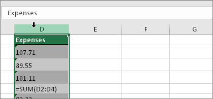
Select a column with this problem. If you don’t want to convert the whole column, you can select one or more cells instead. Just be sure the cells you select are in the same column, otherwise this process won’t work. (See «Other ways to convert» below if you have this problem in more than one column.)
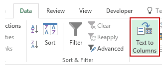
2. Click this button
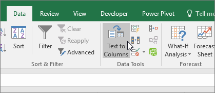
The Text to Columns button is typically used for splitting a column, but it can also be used to convert a single column of text to numbers. On the Data tab, click Text to Columns.
3. Click Apply
The rest of the Text to Columns wizard steps are best for splitting a column. Since you’re just converting text in a column, you can click Finish right away, and Excel will convert the cells.
4. Set the format

Press CTRL + 1 (or  + 1 on the Mac). Then select any format.
Note: If you still see formulas that are not showing as numeric results, then you may have Show Formulas turned on. Go to the Formulas tab and make sure Show Formulas is turned off.
Other ways to convert:
You can use the VALUE function to return just the numeric value of the text.
1. Insert a new column
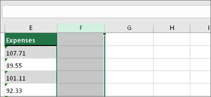
Insert a new column next to the cells with text. In this example, column E contains the text stored as numbers. Column F is the new column.
2. Use the VALUE function
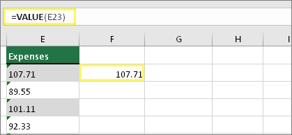
In one of the cells of the new column, type =VALUE() and inside the parentheses, type a cell reference that contains text stored as numbers. In this example it’s cell E23.
3. Rest your cursor here
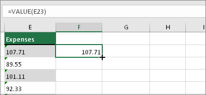
Now you’ll fill the cell’s formula down, into the other cells. If you’ve never done this before, here’s how to do it: Rest your cursor on the lower-right corner of the cell until it changes to a plus sign.
4. Click and drag down
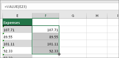
Click and drag down to fill the formula to the other cells. After that’s done, you can use this new column, or you can copy and paste these new values to the original column. Here’s how to do that: Select the cells with the new formula. Press CTRL + C. Click the first cell of the original column. Then on the Home tab, click the arrow below Paste, and then click Paste Special > Values.
If the steps above didn’t work, you can use this method, which can be used if you’re trying to convert more than one column of text.
Select a blank cell that doesn’t have this problem, type the number 1 into it, and then press Enter.
Press CTRL + C to copy the cell.
Select the cells that have numbers stored as text.
On the Home tab, click Paste > Paste Special.
Click Multiply, and then click OK. Excel multiplies each cell by 1, and in doing so, converts the text to numbers.
Press CTRL + 1 (or + 1 on the Mac). Then select any format.
Источник
Available number formats in Excel
In Excel, you can format numbers in cells for things like currency, percentages, decimals, dates, phone numbers, or social security numbers.

Select a cell or a cell range.
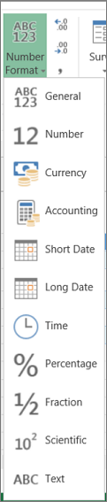
On the Home tab, select Number from the drop-down.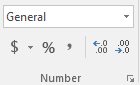
Or, you can choose one of these options:
Press CTRL + 1 and select Number.
Right-click the cell or cell range, select Format Cells… , and select Number.
Select the small arrow, dialog box launcher, and then select Number.
Select the format you want.
Number formats
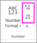
To see all available number formats, click the Dialog Box Launcher next to Number on the Home tab in the Number group.

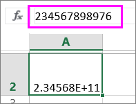
The default number format that Excel applies when you type a number. For the most part, numbers that are formatted with the General format are displayed just the way you type them. However, if the cell is not wide enough to show the entire number, the General format rounds the numbers with decimals. The General number format also uses scientific (exponential) notation for large numbers (12 or more digits).
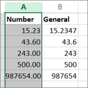
Used for the general display of numbers. You can specify the number of decimal places that you want to use, whether you want to use a thousands separator, and how you want to display negative numbers.
Used for general monetary values and displays the default currency symbol with numbers. You can specify the number of decimal places that you want to use, whether you want to use a thousands separator, and how you want to display negative numbers.
Also used for monetary values, but it aligns the currency symbols and decimal points of numbers in a column.
Displays date and time serial numbers as date values, according to the type and locale (location) that you specify. Date formats that begin with an asterisk ( *) respond to changes in regional date and time settings that are specified in Control Panel. Formats without an asterisk are not affected by Control Panel settings.
Displays date and time serial numbers as time values, according to the type and locale (location) that you specify. Time formats that begin with an asterisk ( *) respond to changes in regional date and time settings that are specified in Control Panel. Formats without an asterisk are not affected by Control Panel settings.
Multiplies the cell value by 100 and displays the result with a percent ( %) symbol. You can specify the number of decimal places that you want to use.
Displays a number as a fraction, according to the type of fraction that you specify.
Displays a number in exponential notation, replacing part of the number with E+n, where E (which stands for Exponent) multiplies the preceding number by 10 to the nth power. For example, a 2-decimal Scientific format displays 12345678901 as 1.23E+10, which is 1.23 times 10 to the 10th power. You can specify the number of decimal places that you want to use.
Treats the content of a cell as text and displays the content exactly as you type it, even when you type numbers.
Displays a number as a postal code (ZIP Code), phone number, or Social Security number.
Allows you to modify a copy of an existing number format code. Use this format to create a custom number format that is added to the list of number format codes. You can add between 200 and 250 custom number formats, depending on the language version of Excel that is installed on your computer. For more information about custom formats, see Create or delete a custom number format.
You can apply different formats to numbers to change how they appear. The formats only change how the numbers are displayed and don’t affect the values. For example, if you want a number to show as currency, you’d click the cell with the number value > Currency.
Applying a number format only changes how the number is displayed and doesn’t affect cell values that’s used to perform calculations. You can see the actual value in the formula bar.

Here’s a list of available number formats and how you can use them in Excel for the web:
Default number format. If the cell isn’t wide enough to show the entire number, this format rounds the number. For example, 25.76 shows as 26.
Also, if the number is 12 or more digits, General format displays the value with scientific (exponential) notation.
Works very much like the General format but varies how it shows numbers with decimal place separators and negative numbers. Here are some examples of how both formats display numbers:
Shows a monetary symbol with numbers. You can specify the number of decimal places with Increase Decimal or Decrease Decimal.
Also used for monetary values, but aligns the currency symbols and decimal points of numbers in a column.
Shows date in this format:
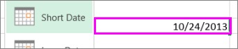
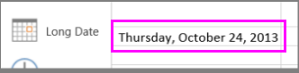
Shows month, day and year in this format:
Shows number date and time serial numbers as time values.
Multiplies the cell value by 100 and displays the result with a percent ( %) symbol.
Use Increase Decimal or Decrease Decimal to specify the number of decimal places you want.
Shows the number as a fraction. For example, 0.5 displays as ½.
Displays numbers in exponential notation, replacing part of the number with E+ n, where E (Exponent) multiplies the preceding number by 10 to the nth power. For example, a 2-decimal Scientific format displays 12345678901 as 1.23E+10, which is 1.23 times 10 to the 10th power. To specify the number of decimal places you want to use, apply Increase Decimal or Decrease Decimal.
Treats the cell value as text and displays it exactly as you type it, even when you type numbers. Learn more about formatting numbers as text.
Need more help?
You can always ask an expert in the Excel Tech Community or get support in the Answers community.
Источник
Convert Text to Numbers in Excel – A Step By Step Tutorial
It’s common to find numbers stored as text in Excel. This leads to incorrect calculations when you use these cells in Excel functions such as SUM and AVERAGE (as these functions ignore cells that have text values in it). In such cases, you need to convert cells that contain numbers as text back to numbers.
Now before we move forward, let’s first look at a few reasons why you may end up with a workbook that has numbers stored as text.
- Using ‘ (apostrophe) before a number.
- A lot of people enter apostrophe before a number to make it text. Sometimes, it’s also the case when you download data from a database. While this makes the numbers show up without the apostrophe, it impacts the cell by forcing it to treat the numbers as text.
- Getting numbers as a result of a formula (such as LEFT, RIGHT, or MID)
- If you extract the numerical part of a text string (or even a part of a number) using the TEXT functions, the result is a number in the text format.
Now, let’s see how to tackle such cases.
Convert Text to Numbers in Excel
In this tutorial, you’ll learn how to convert text to numbers in Excel.
The method you need to use depends on how the number has been converted into text. Here are the ones that are covered in this tutorial.
- Using the ‘Convert to Number’ option.
- Change the format from Text to General/Number.
- Using Paste Special.
- Using Text to Columns.
- Using a Combination of VALUE, TRIM, and CLEAN function.
Convert Text to Numbers Using ‘Convert to Number’ Option
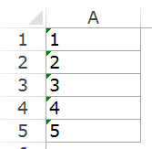
When an apostrophe is added to a number, it changes the number format to text format. In such cases, you’ll notice that there is a green triangle at the top left part of the cell.
In this case, you can easily convert numbers to text by following these steps:
- Select all the cells that you want to convert from text to numbers.

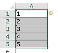
- Click on the yellow diamond shape icon that appears at the top right. From the menu that appears, select ‘Convert to Number’ option.
This would instantly convert all the numbers stored as text back to numbers. You would notice that the numbers get aligned to the right after the conversion (while these were aligned to the left when stored as text).
Convert Text to Numbers by Changing Cell Format
When the numbers are formatted as text, you can easily convert it back to numbers by changing the format of the cells.
Here are the steps:
- Select all the cells that you want to convert from text to numbers.
- Go to Home –> Number. In the Number Format drop-down, select General.
This would instantly change the format of the selected cells to General and the numbers would get aligned to the right. If you want, you can select any of the other formats (such as Number, Currency, Accounting) which will also lead to the value in cells being considered as numbers.
Convert Text to Numbers Using Paste Special Option
To convert text to numbers using Paste Special option:
Convert Text to Numbers Using Text to Column
This method is suitable in cases where you have the data in a single column.
Here are the steps:
- Select all the cells that you want to convert from text to numbers.
- Go to Data –> Data Tools –> Text to Columns.
- In the Text to Column Wizard:
While you may still find the resulting cells to be in the text format, and the numbers still aligned to the left, now it would work in functions such as SUM and AVERAGE.
Convert Text to Numbers Using the VALUE Function
You can use a combination of VALUE, TRIM and CLEAN function to convert text to numbers.
- VALUE function converts any text that represents a number back to a number.
- TRIM function removes any leading or trailing spaces.
- CLEAN function removes extra spaces and non-printing characters that might sneak in if you import the data or download from a database.
Suppose you want convert cell A1 from text to numbers, here is the formula:
If you want to apply this to other cells as well, you can copy and use the formula.
You May Also Like the Following Excel Tutorials:
Источник
In Excel, you can format numbers in cells for things like currency, percentages, decimals, dates, phone numbers, or social security numbers.
-
Select a cell or a cell range.
-
On the Home tab, select Number from the drop-down.
Or, you can choose one of these options:-
Press CTRL + 1 and select Number.
-
Right-click the cell or cell range, select Format Cells… , and select Number.
-
Select the small arrow, dialog box launcher, and then select Number.
-
-
Select the format you want.
Number formats
To see all available number formats, click the Dialog Box Launcher next to Number on the Home tab in the Number group.
|
Format |
Description |
|---|---|
|
General |
The default number format that Excel applies when you type a number. For the most part, numbers that are formatted with the General format are displayed just the way you type them. However, if the cell is not wide enough to show the entire number, the General format rounds the numbers with decimals. The General number format also uses scientific (exponential) notation for large numbers (12 or more digits). |
|
Number |
Used for the general display of numbers. You can specify the number of decimal places that you want to use, whether you want to use a thousands separator, and how you want to display negative numbers. |
|
Currency |
Used for general monetary values and displays the default currency symbol with numbers. You can specify the number of decimal places that you want to use, whether you want to use a thousands separator, and how you want to display negative numbers. |
|
Accounting |
Also used for monetary values, but it aligns the currency symbols and decimal points of numbers in a column. |
|
Date |
Displays date and time serial numbers as date values, according to the type and locale (location) that you specify. Date formats that begin with an asterisk (*) respond to changes in regional date and time settings that are specified in Control Panel. Formats without an asterisk are not affected by Control Panel settings. |
|
Time |
Displays date and time serial numbers as time values, according to the type and locale (location) that you specify. Time formats that begin with an asterisk (*) respond to changes in regional date and time settings that are specified in Control Panel. Formats without an asterisk are not affected by Control Panel settings. |
|
Percentage |
Multiplies the cell value by 100 and displays the result with a percent (%) symbol. You can specify the number of decimal places that you want to use. |
|
Fraction |
Displays a number as a fraction, according to the type of fraction that you specify. |
|
Scientific |
Displays a number in exponential notation, replacing part of the number with E+n, where E (which stands for Exponent) multiplies the preceding number by 10 to the nth power. For example, a 2-decimal Scientific format displays 12345678901 as 1.23E+10, which is 1.23 times 10 to the 10th power. You can specify the number of decimal places that you want to use. |
|
Text |
Treats the content of a cell as text and displays the content exactly as you type it, even when you type numbers. |
|
Special |
Displays a number as a postal code (ZIP Code), phone number, or Social Security number. |
|
Custom |
Allows you to modify a copy of an existing number format code. Use this format to create a custom number format that is added to the list of number format codes. You can add between 200 and 250 custom number formats, depending on the language version of Excel that is installed on your computer. For more information about custom formats, see Create or delete a custom number format. |
You can apply different formats to numbers to change how they appear. The formats only change how the numbers are displayed and don’t affect the values. For example, if you want a number to show as currency, you’d click the cell with the number value > Currency.
Applying a number format only changes how the number is displayed and doesn’t affect cell values that’s used to perform calculations. You can see the actual value in the formula bar.
Here’s a list of available number formats and how you can use them in Excel for the web:
|
Number format |
Description |
|---|---|
|
General |
Default number format. If the cell isn’t wide enough to show the entire number, this format rounds the number. For example, 25.76 shows as 26. Also, if the number is 12 or more digits, General format displays the value with scientific (exponential) notation.
|
|
Number |
Works very much like the General format but varies how it shows numbers with decimal place separators and negative numbers. Here are some examples of how both formats display numbers:
|
|
Currency |
Shows a monetary symbol with numbers. You can specify the number of decimal places with Increase Decimal or Decrease Decimal.
|
|
Accounting |
Also used for monetary values, but aligns the currency symbols and decimal points of numbers in a column. |
|
Short Date |
Shows date in this format:
|
|
Long Date |
Shows month, day and year in this format:
|
|
Time |
Shows number date and time serial numbers as time values. |
|
Percentage |
Multiplies the cell value by 100 and displays the result with a percent (%) symbol. Use Increase Decimal or Decrease Decimal to specify the number of decimal places you want.
|
|
Fraction |
Shows the number as a fraction. For example, 0.5 displays as ½. |
|
Scientific |
Displays numbers in exponential notation, replacing part of the number with E+n, where E (Exponent) multiplies the preceding number by 10 to the nth power. For example, a 2-decimal Scientific format displays 12345678901 as 1.23E+10, which is 1.23 times 10 to the 10th power. To specify the number of decimal places you want to use, apply Increase Decimal or Decrease Decimal. |
|
Text |
Treats the cell value as text and displays it exactly as you type it, even when you type numbers. Learn more about formatting numbers as text. |
It’s common to find numbers stored as text in Excel. This leads to incorrect calculations when you use these cells in Excel functions such as SUM and AVERAGE (as these functions ignore cells that have text values in it). In such cases, you need to convert cells that contain numbers as text back to numbers.
Now before we move forward, let’s first look at a few reasons why you may end up with a workbook that has numbers stored as text.
- Using ‘ (apostrophe) before a number.
- A lot of people enter apostrophe before a number to make it text. Sometimes, it’s also the case when you download data from a database. While this makes the numbers show up without the apostrophe, it impacts the cell by forcing it to treat the numbers as text.
- Getting numbers as a result of a formula (such as LEFT, RIGHT, or MID)
- If you extract the numerical part of a text string (or even a part of a number) using the TEXT functions, the result is a number in the text format.
Now, let’s see how to tackle such cases.
Convert Text to Numbers in Excel
In this tutorial, you’ll learn how to convert text to numbers in Excel.
The method you need to use depends on how the number has been converted into text. Here are the ones that are covered in this tutorial.
- Using the ‘Convert to Number’ option.
- Change the format from Text to General/Number.
- Using Paste Special.
- Using Text to Columns.
- Using a Combination of VALUE, TRIM, and CLEAN function.
Convert Text to Numbers Using ‘Convert to Number’ Option
When an apostrophe is added to a number, it changes the number format to text format. In such cases, you’ll notice that there is a green triangle at the top left part of the cell.
In this case, you can easily convert numbers to text by following these steps:
- Select all the cells that you want to convert from text to numbers.

- Click on the yellow diamond shape icon that appears at the top right. From the menu that appears, select ‘Convert to Number’ option.
This would instantly convert all the numbers stored as text back to numbers. You would notice that the numbers get aligned to the right after the conversion (while these were aligned to the left when stored as text).
Convert Text to Numbers by Changing Cell Format
When the numbers are formatted as text, you can easily convert it back to numbers by changing the format of the cells.
Here are the steps:
- Select all the cells that you want to convert from text to numbers.
- Go to Home –> Number. In the Number Format drop-down, select General.
This would instantly change the format of the selected cells to General and the numbers would get aligned to the right. If you want, you can select any of the other formats (such as Number, Currency, Accounting) which will also lead to the value in cells being considered as numbers.
Also read: How to Convert Serial Numbers to Dates in Excel
Convert Text to Numbers Using Paste Special Option
To convert text to numbers using Paste Special option:
Convert Text to Numbers Using Text to Column
This method is suitable in cases where you have the data in a single column.
Here are the steps:
- Select all the cells that you want to convert from text to numbers.
- Go to Data –> Data Tools –> Text to Columns.

- In the Text to Column Wizard:
While you may still find the resulting cells to be in the text format, and the numbers still aligned to the left, now it would work in functions such as SUM and AVERAGE.
Convert Text to Numbers Using the VALUE Function
You can use a combination of VALUE, TRIM and CLEAN function to convert text to numbers.
- VALUE function converts any text that represents a number back to a number.
- TRIM function removes any leading or trailing spaces.
- CLEAN function removes extra spaces and non-printing characters that might sneak in if you import the data or download from a database.
Suppose you want convert cell A1 from text to numbers, here is the formula:
=VALUE(TRIM(CLEAN(A1)))
If you want to apply this to other cells as well, you can copy and use the formula.
Finally, you can convert the formula to value using paste special.
You May Also Like the Following Excel Tutorials:
- Multiply in Excel Using Paste Special.
- How to Convert Text to Date in Excel (8 Easy Ways)
- How to Convert Numbers to Text in Excel
- Convert Formula to Values Using Paste Special.
- Excel Custom Number Formatting.
- Convert Time to Decimal Number in Excel
- Change Negative Number to Positive in Excel
- How to Capitalize First Letter of a Text String in Excel
- Convert Scientific Notation to Number or Text in Excel
- How To Convert Date To Serial Number In Excel?
This post is going to show you all the ways you can convert text to numbers in Microsoft Excel.
An issue that comes up quite often in Excel is numbers that have been entered or formatted as text values.
This can cause many headaches when trying to troubleshoot why a formula like a SUM is not giving the correct answer.
Even though the data looks like a number, it can actually be a text value and will be ignored from any numerical calculations like a sum.
In this post, I will show you how you can identify such numbers which are stored as text values, and 7 ways you can use to convert the text into a proper number value.
How to Indentify Numbers Entered as Text
How can you tell if your number data has been entered as text?
There are quite a few easy ways to tell!
Left Aligned
The first way you might be able to tell if you have text values instead of numerical values is the way the data is aligned in the cell.
By default text is left aligned and numbers are right aligned.
Unless the alignment formatting has been changed from the default, this will be an easy way to spot numbers that have been formatted as text.
Green Triangle Error Checking
If you don’t realize you have numbers entered as text values, it can potentially cause some serious errors. This is why it’s flagged by Excel’s built-in error checker.
Any cells that are flagged with an error will show a small green triangle in the left of the cell to visually indicate an error.
When you select such a cell a small warning icon will appear.
When you click on this, it will show you what the error is. In this case, you can see the error is Number Stored as Text.
You can turn off this error checking entirely, or customize which errors are flagged.
Go to the File tab and then select Options at the bottom. This will open up the Excel Options menu.
In the Formula section of the Excel Options menu ➜ Error Checking.
Uncheck the Enable background error checking option to disable this feature. You can also customize the color used to indicate errors here.
Text Format Applied
One way that numbers get entered as text is when the cell has been formatted as text. This causes values to be entered as text values regardless of whether they are numerical.
There is a quick way to determine whether or not a cell has had text formatting applied.
Select the cell and go to the Home tab. You will be able to see if Text is the selected formatting in the dropdown menu found in the Number section of the ribbon.
Preceding Apostrophe
Another way that numbers can be entered as text is by using a preceding apostrophe.
When you enter an apostrophe ' as the first character in a cell, anything after will be regarded as a text value by Excel.
This means if you see a leading apostrophe in the formula bar, you know the data is a text value.
Use the ISTEXT Function
Excel has a function you can use to test if a value is a text value or not.
ISTEXT ( input )- input is the value, cell or range which you want to test if it is text.
The ISTEXT function will return TRUE if the value is text and FALSE otherwise.
= ISTEXT ( B3 )Here you can see the ISTEXT function being used to determine if the cells contain text. The function returns TRUE when it finds a text value.
ISNUMBER ( input )- input is the value, cell or range which you want to test if it is a number.
Similarly, you can test if a value is a number using the ISNUMBER function. It takes a single input and returns TRUE when the value is a number and FALSE otherwise.
Here the same data is tested using the ISNUMBER function. The function returns FALSE when it does not find a number.
Status Bar Only Shows a Count
Another way to quickly test a range of cells to see if they are all text is by using the status bar.
When you select a range of numerical values, Excel will show you some basic statistics like the sum, min, max, and average in the status bar.
If they are all numbers entered as text values, then these basic statistics won’t be calculated. Instead, you will only see the count of the cells in the status bar.
Note: If just one of the cells is a numerical value, you will see the full set of statistics in the status bar.
Convert Text to Number with Error Checking
You have already seen that you can use error checking to spot numbers entered as text.
The error checking will also allow you to convert these text values into proper numbers.
Click on the Error icon and choose Convert to Number from the options. Excel will then convert each cell in the selected range into a number.
Note: This option can be very slow when you have a large number of cells to convert.
Convert Text to Number with Text to Column
Usually, Text to Columns is for splitting data into multiple columns. But with this trick, you can use it to convert text format into the general format.
Text to Column will let you choose a delimiter character to split your data based on. If you deselect this option and don’t pick any delimiter then it won’t split your data.
You are then able to choose how to format the results, and this is where you can choose a general format for the output.
Follow these steps to use the text to column feature to convert text to numbers.
- Select the cells that contain the text which you want to convert into number.
- Go to the Data tab.
- Click on the Text to Column command found in the Data Tools tab.
- Select Delimited in the Original data type options.
- Press the Next button.
- Press the Next button again in step 2 of the Convert Text to Columns wizard. You can keep the default options.
- Select General from the Column data format option.
- Select a Destination if you want to place the converted values in a new location. Otherwise you can keep the default value which should be the active cell, this will replace the text with numeric values.
- Press the Finish button.
This will convert your text values into numerical values.
The Text to Column command is usually used to split comma-separated or other delimiter separated data into multiple columns.
Any delimited data will be text data, so when Excel splits the data into multiple columns it also converts numerical data into numbers for added convenience.
This is also true even if there is nothing to split!
So the Text to Column wizard can be used to converts numerical text values to numbers.
Convert Text to Number with Multiply by 1
Even when values are stored as text you can still perform certain numerical calculations with them and the results of these calculations will also be numerical values.
You can use this to convert the text into numbers by multiplying them by 1. Since you are multiplying by 1, it won’t change the numbers but it will convert them.
= B3 * 1You can use the above formula in an adjacent cell and copy and paste it down to convert an entire column.
If you want to remove the formula after, you can copy and paste them as values.
Convert Text to Number with Paste Special Multiply
Multiplying by 1 is a great trick for converting text to values, but you might not want to use a formula for this.
The great news is there is an easy way to multiply your text by 1 without using a formula.
This means you can convert your text in place and you don’t need to copy and paste formulas as values in an additional step.
You can use Paste Special Multiply to convert your text values. Follow these steps to multiply by 1 using Paste Special.
- Enter 1 into a cell elsewhere in the sheet. The 1 doesn’t even need to be a number value and can be a text value.
- Copy the cell which contains 1 using Ctrl + C on your keyboard or right click and choose Copy.
- Select the cells with the text values to convert.
- Press Ctrl + Alt + V on your keyboard or right click and choose Paste Special. This will open up the Paste Special menu.
- Select Values under the Paste options and select Multiply under the Operation options.
- Press the OK button.
This will multiply all the values by 1 which was the value in the copied cell. As a result, the text is converted into values, but since you are multiplying by 1 the numbers won’t change.
Convert Text to Number with VALUE Function
There is actually a dedicated function you can use for converting text to numerical values.
The VALUE function takes a text value and returns the text value as a number.
= VALUE ( text )- text is the text value you want to convert into a numerical value.
If the text contains any non-numerical characters, then the VALUE function will return a #VALUE! error. It doesn’t extract numbers from text, it can only convert numbers entered as text into numbers.
= VALUE ( B3 )You can use the above formula to convert the text in cell B3 into a number and then copy and paste the formula to convert the entire column.
Convert Text to Number with Power Query
Power Query is an amazing tool for any type of data transformation required. It can certainly be used to convert text into numbers as well.
Power Query is strongly typed. This means calculations with incompatible data types will result in an error. So you won’t be able to multiply text values by 1 to convert them into numbers.
But Power Query does come with an easy way to convert data types, including text to numbers.
Follow these steps once your data has been imported into Power Query.
Click on the data type icon to the left side of the column heading for the values you want to convert.
Each column in the Power Query editor has a data type icon that displays the current data type of the column. If the column has not been assigned a data type, then the icon shown will be ABC123.
There are several numeric data types available in Power Query and which one you choose will depend on the level of decimal precision you need.
In this case, you can select the Whole Number option from the menu.
Notice the values in the column are now right-aligned and the data type icon has changed? These are visual indicators that the data type is now whole numbers instead of text.
= Table.TransformColumnTypes(Source,{{"Text", Int64.Type}})You will see a new Changed Type step has been applied to the query and it will use the above M code formula.
You can then press the Close & Load button in the Home tab to save the results and load the data into Excel.
You might not even need to apply this data type conversion step to your query. When you first import data into Power Query, it will usually guess the data type and apply the conversion for you!
Convert Text to Number with Power Pivot
If you want to analyze or summarize your data after you convert it from text to numbers, then you might want to do the conversion in Power Pivot.
Power Pivot is an add-in that allows you to efficiently analyze millions of rows in the data model with Pivot Tables.
With Power Pivot, you can build row-level calculations using the DAX formula language to create new columns in your datasets. You can then access these new columns in your pivot tables connected to the data model.
In this case, the DAX formula you can use to convert text to numbers is the exact same as the formula in the grid.
Follow these steps inside the Power Pivot add-in to create a new calculated column that converts the text to numbers.
Select any cell under the Add Column heading.
=VALUE(TextNumbers[Text])Insert the above formula. TextNumbers is the name of the table of data in Power Pivot and Text is the name of the column you want to convert.
Double click on the column heading to change the name.
Press the Save icon and close the Power Pivot add-in.
Now you can create a pivot table from the data model and this new column will be available for use inside the pivot table just like any other field.
- Go to the Insert tab.
- Click on the PivotTable button.
- Choose From Data Model in the available options.
The calculated column will be available in your pivot table fields list and you will be able to use it like any other number field.
Conclusions
There are many reasons why you might have data that contains numbers formatted as text.
If you want to freely use these values in your calculations, you will need to convert them into numbers.
Thankfully, there are many easy options to convert text to numbers such as error checking, paste special, basic multiplication, and the VALUE function. These are all easy ways to convert text inside the grid.
If you’re importing your data using Power Query or Power Pivot, you can perform the conversion inside each of these tools. Both have methods available to convert text to numbers.
Do you use any of these methods to change your text values to numbers? Do you know any other interesting ways to perform this action? Let me know in the comments below!
About the Author
John is a Microsoft MVP and qualified actuary with over 15 years of experience. He has worked in a variety of industries, including insurance, ad tech, and most recently Power Platform consulting. He is a keen problem solver and has a passion for using technology to make businesses more efficient.
Numbering in Excel means providing a cell with numbers like serial numbers to some table. We can also do it manually by filling the first two cells with numbers and dragging them down to the end of the table, which Excel will automatically load the series. Else, we can use the =ROW() formula to insert a row number as the serial number in the data or table.
When working with Excel, some small tasks need to be done repeatedly. However, if we know the right way to do it, they can save a lot of time. For example, generating the numbers in Excel is a task that is often used while working. Serial numbers play a very important role in Excel. It defines a unique identity for each record of your data.
One of the ways is to add the serial numbers manually in Excel. But it can be a pain if you have the data of hundreds or thousands of rows and must enter the row number for them.
This article will cover the different ways to do it.
Table of contents
- Numbering in Excel
- How to Add Serial Number in Excel Automatically?
- #1 – Using Fill Handle
- #2 – Using Fill Series
- #3 – Using the ROW Function
- Things to Remember about Numbering in Excel
- Recommended Articles
How to Add Serial Number in Excel Automatically?
There are many ways to generate the number of rows in Excel.
You can download this Numbering in Excel Template here – Numbering in Excel Template
- Using Fill Handle
- Using Fill Series
- Using ROW Function
#1 – Using Fill Handle
It identifies a pattern from a few already filled cells and then quickly uses that pattern to fill the entire column.
For example, let us take the below dataset.
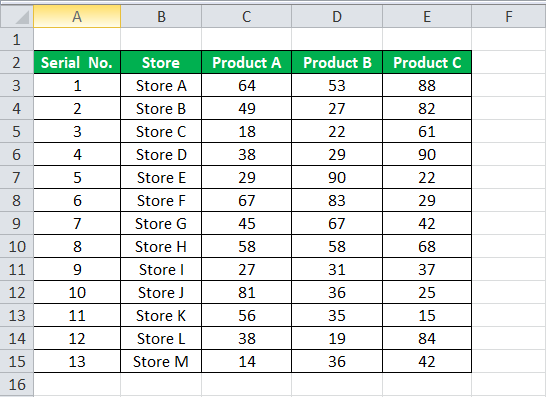
For the above dataset, we have to fill the serial no record-wise. Follow the below steps:
- First, we must enter 1 in cell A3 and insert 2 in cell A4.
- Then, select both the cells as per the below screenshot.

As we can see, a small square is shown in the above screenshot, which is rounded by a red color called “Fill Handle” in Excel.
Place the mouse cursor on this square and double-click on the fill handle.
- It will automatically fill all the cells until the end of the dataset. For example, refer to the below screenshot.

As the fill handle identifies the pattern, fill the individual cells with that pattern.
If you have any blank row in the dataset, the fill handle would only work until the last contiguous non-blank row.

#2 – Using Fill Series
It gives more control over data on how the serial numbers are entered into Excel.
For example, suppose you have below the score of students subject-wise.

Follow the below steps to fill series in the Excel:
- We must first insert 1 in cell A3.
- Then, go to the “HOME” tab. Next, click on the “Fill” option under the “Editing” section, as shown in the below screenshot.

- Click on the “Fill” dropdown. It has many options. Click on “Series,” as shown in the below screenshot.

- It will open a dialog box, as shown below screenshot.

- Click on “Columns” under the “Series in” section. Then, refer to the below screenshot.

- Insert the value under the “Stop value” field. In this case, we have 10 records; enter 10. If we skip this value, the Fill “Series” option may not work.
- Enter “OK.” It will fill rows with serial numbers from 1 to 10. Refer to the below screenshot.

#3 – Using the ROW Function
Excel has a built-in function, which also can be used to number the rows in Excel. To get the Excel row numbering, we must enter the following formula in the first cell shown below:

- The ROW function gives the Excel row number of the current row. We have subtracted 3 from it as we started the data from the 4th. If the data starts from the 2nd row, we must remove 1 from it.
- See the below screenshot. Using =ROW()-3 formula.

Drag this formula for the rest of the rows. The final result is shown below.
Using this formula for numbering will not damage the numbers if we delete a record in the dataset. Furthermore, since the ROW function does not reference cell addresses, it will automatically adjust to give the correct row number.
Things to Remember about Numbering in Excel
- The “Fill Handle” and “Fill Series” options are static. Therefore, if we move or delete any record or row in the dataset, the row number will not change accordingly.
- The ROW function gives the exact numbering if we cut and copy the data in Excel.
Recommended Articles
This article is a guide to Numbering in Excel. We discuss how to automatically add serial numbers in Excel using the fill handle, fill series, and ROW function, along with examples and downloadable templates. You may learn more about Excel functions from the following articles: –
- Auto Numbering in ExcelThere are two approaches for auto numbering. To begin, fill the first two cells with the series you wish to insert and drag it to the table’s end. Second, use the =ROW() formula to get the number, and then drag it to the table’s end.read more
- Row Limit in Excel
- Excel Negative NumberIn Excel, negative numbers, i.e. numbers less than 0 in value, are displayed with minus symbols by default.read more
- IsNumber FunctionISNUMBER function in excel is an information function that checks if the referred cell value is numeric or non-numeric.read more
- Null in ExcelNull is a type of error in Excel that occurs when two or more cell references provided in formulas are wrong, or when their position is incorrect. Using space in formulas between two cell references, for example, will result in a null error.read more
Reader Interactions