
Excel for Microsoft 365 Excel 2021 Excel 2019 Excel 2016 Excel 2013 Excel 2010 Excel 2007 More…Less
Unlike other Microsoft Office programs, such as Word, Excel does not provide a button that you can use to highlight all or individual portions of data in a cell.
However, you can mimic highlights on a cell in a worksheet by filling the cells with a highlighting color. For a fast way to mimic a highlight, you can create a custom cell style that you can apply to fill cells with a highlighting color. Then, after you apply that cell style to highlight cells, you can quickly copy the highlighting to other cells by using Format Painter.
If you want to make specific data in a cell stand out, you can display that data in a different font color or format.
Create a cell style to highlight cells
-
Click Home > New Cell Styles.
Notes:
-
If you don’t see Cell Style, click the More
 button next to the cell style gallery.
 -
-
-
In the Style name box, type an appropriate name for the new cell style.
Tip: For example, type Highlight.
-
Click Format.
-
In the Format Cells dialog box, on the Fill tab, select the color that you want to use for the highlight, and then click OK.
-
Click OK to close the Style dialog box.
The new style will be added under Custom in the cell styles box.
-
On the worksheet, select the cells or ranges of cells that you want to highlight. How to select cells?
-
On the Home tab, in the Styles group, click the new custom cell style you created.
Note: Custom cell styles are displayed at the top of the list of cell styles. If you see the cell styles box in the Styles group, and the new cell style is one of the first six cell styles on the list, you can click that cell style directly in the Styles group.
Use Format Painter to apply a highlight to other cells
-
Select a cell that is formatted with the highlight that you want to use.
-
On the Home tab, in the Clipboard group, double-click Format Painter
, and then drag the mouse pointer across as many cells or ranges of cells that you want to highlight. -
When you’re done, click Format Painter again or press ESC to turn it off.
Display specific data in a different font color or format
-
In a cell, select the data that you want to display in a different color or format.
How to select data in a cell
To select the contents of a cell
Do this
In the cell
Double-click the cell, and then drag across the contents of the cell that you want to select.
In the formula bar
Click the cell, and then drag across the contents of the cell that you want to select in the formula bar.
By using the keyboard
Press F2 to edit the cell, use the arrow keys to position the insertion point, and then press SHIFT+ARROW key to select the contents.
-
On the Home tab, in the Font group, do one of the following:
-
To change the text color, click the arrow next to Font Color
and then, under Theme Colors or Standard Colors, click the color that you want to use. -
To apply the most recently selected text color, click Font Color
. -
To apply a color other than the available theme colors and standard colors, click More Colors, and then define the color that you want to use on the Standard tab or Custom tab of the Colors dialog box.
-
To change the format, click Bold
, Italic , or Underline .Keyboard shortcut You can also press CTRL+B, CTRL+I, or CTRL+U.
-
Need more help?
Colorize your data for maximum impact
Updated on November 11, 2021
What to Know
- To highlight: Select a cell or group of cells > Home > Cell Styles, and select the color to use as the highlight.
- To highlight text: Select the text > Font Color and choose a color.
- To create a highlight style: Home > Cell Styles > New Cell Style. Enter a name, select Format > Fill, choose color > OK.
This article explains how to highlight in Excel. Additional instructions cover how to create a customized highlight style. Instructions apply to Excel 2019, 2016, and Excel for Microsoft 365.
Why Highlight?
Choosing to highlight cells in Excel can be a great way to make sure data or words stand out or increase readability within a file with a lot of information. You can select both cells and text as a highlight in Excel, and you can also customize the colors to suit your needs. Here’s how to highlight in Excel.
How to Highlight Cells in Excel
Spreadsheet cells are the boxes that contain text within a Microsoft Excel document, though many are also completely empty. Both empty and filled Excel cells can be customized in a variety of different ways, including being given a colored highlight.
-
Open the Microsoft Excel document on your device.
-
Select a cell you want to highlight.
To select a group of cells in Excel, select one, press Shift, then select another. Alternatively, you can select individual cells that are separate from each other by holding down Ctrl while you select them.
-
From the top menu, select Home, followed by Cell Styles.
-
A menu with a variety of cell color options pops up. Hover your mouse cursor over each color to see a live preview of the cell color change in the Excel file.
-
When you find a highlight color that you like, select it to apply the change.
If you change your mind, press Ctrl+Z to undo the cell highlight.
-
Repeat for any other cells that you want to apply a highlight to.
To select all of the cells in a column or row, select the numbers on the side of the document or the letters at the top.
How to Highlight Text in Excel
If you just want to highlight text in Excel instead of the entire cell, you can do that too. Here’s how to highlight in Excel when you just want to change the color of the words in the cell.
-
Open your Microsoft Excel document.
-
Double-click the cell containing text you want to format.
-
Press the left mouse button and drag it across the words you want to colorize to highlight them. A small menu appears.
-
Select the Font Color icon in the small menu to use the default color option or select the arrow next to it to choose a custom color.
You can also use this menu to apply bold or italics style options as you would in Microsoft Word and other text editor programs.
-
Select a text color from the pop-up color palette.
-
The color is applied to the selected text. Select elsewhere in the Excel document to deselect the cell.
How to Create a Microsoft Excel Highlight Style
There are a lot of default cell style options in Microsoft Excel. However, if you don’t like any of the available choices, you can create your own personal style.
-
Open a Microsoft Excel document.
-
Select Home, followed by Cell Styles.
-
Select New Cell Style.
-
Enter a name for the new cell style and then select Format.
-
Select Fill in the Format Cells window.
-
Choose a fill color from the palette. Choose the Alignment, Font or Border tabs to make other changes to the new style and then select OK to save it.
You should now see your custom cell style at the top of the Cell Styles menu.
Thanks for letting us know!
Get the Latest Tech News Delivered Every Day
Subscribe
In a cell select the data that you want to display in a different color or format. Double-click the cell and then drag across the contents of the cell that you want to select. Click the cell and then drag across the contents of the cell that you want to select in the formula bar.
How do you highlight specific data in Excel?
Select the range of cells the table or the whole sheet that you want to apply conditional formatting to. On the Home tab click Conditional Formatting point to Highlight Cells Rules and then click Text that Contains. In the box next to containing type the text that you want to highlight and then click OK.
How do you quickly highlight in Excel?
Press and hold the Shift key on the keyboard. Press and release the Spacebar key on the keyboard. Release the Shift key. All cells in the selected row are highlighted including the row header.
How do I highlight a cell in Excel?
- Press F5 key then a searching box pops out for you to type the specified value you search.
- Click OK the matched results have been highlighted with a background color. …
- If there is no matched value found a dialog pops out to remind you.
How do you highlight text in an Excel cell?
Apply conditional formatting based on text in a cell
- Select the cells you want to apply conditional formatting to. Click the first cell in the range and then drag to the last cell.
- Click HOME > Conditional Formatting > Highlight Cells Rules > Text that Contains. …
- Select the color format for the text and click OK.
See also what factors affect the rate of erosion
What is the shortcut key for highlight?
Adding highlighting: Select the text you want to highlight then press Ctrl+Alt+H. Removing highlighting: Select the highlighted text then press Ctrl+Alt+H.
Is there a shortcut key for highlighting in Excel?
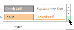
With the cells selected press Alt+H+H. Use the arrow keys on the keyboard to select the color you want. The arrow keys will move a small orange box around the selected color.
How do I highlight in Excel without a mouse?
If you hold down the shift key and then press an arrow key you can extend this selection in any direction without using the mouse. To select an entire column press control-spacebar. Once you have the column selected you can press shift and extend the selection to the right or the left using the arrow keys.
How do I highlight all the values in a column in Excel?
Select the letter at the top to select the entire column. Or click on any cell in the column and then press Ctrl + Space.
How do you highlight cells based on a list?
Highlight Items From a List
- Create a list of items you want to highlight. …
- Select range A2:A7.
- On the Ribbon’s Home tab click Conditional Formatting then click New Rule.
- Click Use a Formula to Determine Which Cells to Format. …
- For the formula enter. …
- Click the Format button.
- Select a font colour for highlighting.
How do I highlight a column in Excel?
Let’s see how easy is selecting columns in excel.
- Select any cell in any column.
- Press Ctrl + Space shortcut keys on the keyboard. The whole column will be highlighted in excel to show the selected column as shown below in the picture. You can also say that this is a shortcut to highlight column in excel.
How do I automatically color a cell in Excel?
In the menu choose Format – Conditional Formatting. In the Conditional Formatting box choose Formula Is. In the text box enter the cell reference of the FIRST table (eg C4=”4+”) do not enter any $ symbols. Click the Format button and select the background fill to match the one in the first table.
How do you highlight yellow in Excel?
Create a cell style to highlight cells
Click Format. In the Format Cells dialog box on the Fill tab select the color that you want to use for the highlight and then click OK. Click OK to close the Style dialog box. The new style will be added under Custom in the cell styles box.
How do you highlight using Ctrl?
If you want to highlight one word at a time press Ctrl while holding down Shift and then press the Left arrow or Right arrow . If you want to highlight a whole line of text move your cursor to the start of the line hold the Shift key and then press the Down arrow .
What are the 20 shortcut keys?
Basic Windows keyboard shortcuts
- Ctrl+Z: Undo. No matter what program you’re running Ctrl+Z will roll back your last action. …
- Ctrl+W: Close. …
- Ctrl+A: Select all. …
- Alt+Tab: Switch apps. …
- Alt+F4: Close apps. …
- Win+D: Show or hide the desktop. …
- Win+left arrow or Win+right arrow: Snap windows. …
- Win+Tab: Open the Task view.
See also how to learn cherokee
What is Ctrl R in Excel?
Ctrl+R in Excel and other spreadsheet programs
In Microsoft Excel and other spreadsheet programs pressing Ctrl+R fills the row cell to the right with the contents of the selected cell. To fill more than one cell select the source cell and press Ctrl+Shift+Right arrow to select multiple cells.
Why is Excel not letting me highlight cells?
To work around this issue use one of the following methods: Do not clear the Select Locked Cells check box when you protect a worksheet: Start Excel open your workbook and then select the range that you want to allow access to. … Click Protect Sheet leave the Select Locked Cells check box selected and then click OK.
How do you highlight a large amount of cells in Excel?
Select a Large Range of Cells With the Shift Key
Click the first cell in the range you want to select. Scroll your sheet until you find the last cell in the range you want to select. Hold down your Shift key and then click that cell. All the cells in the range are now selected.
How do I automatically highlight rows in Excel?
In the format cells window switch to the fill tab and choose the color you want to use as the color to highlight the active row. Then click OK on the Format Cells window and OK on the New Formatting Rule window. At this point Row 1 should be highlighted with the color you selected.
How do I color code in Excel based on value?
Choose a range of numbers and then select Home Conditional Formatting Color Scale. Choose one of the built-in three-color choices. Using a color scale the numbers are assigned various shades of red yellow and green based on the number selected.
How do you highlight cells in Excel that match a list?
On the Home tab click Conditional Formatting in the Styles group. Choose Highlight Cells Rules and then select Duplicates Values in the subsequent menu (Figure A). In the resulting dialog select an appropriate format and click OK.
How do you highlight 3 columns in Excel?
What is the shortcut key to highlight the entire columns?
Ctrl+Space is the keyboard shortcut to select an entire column.
How do I color a cell in Excel formula?
Re: RE: How do I make excel change the colour of a cell depending on a different cells date?
- Select cell A2.
- click Conditional Formatting on the Home ribbon.
- click New Rule.
- click Use a formula to determine which cells to format.
- click into the formula box and enter the formula. …
- click the Format button and select a red color.
Where is the highlighter tool in Excel?
You find Excel’s highlight function under the “Conditional Formatting” button in the Styles section under the Home tab. When you click it a drop-down menu appears with a “Highlight Cell Rules” option.
How do you highlight text?
Highlight selected text
- Select the text that you want to highlight.
- Go to Home and select the arrow next to Text Highlight Color.
- Select the color that you want. Note: Use a light highlight color if you plan to print the document by using a monochrome palette or printer.
See also What Is A Single Celled Organism?
What are the 10 shortcut keys?
Below are the top 10 keyboard shortcuts we recommend everyone memorize and use.
- Ctrl+C or Ctrl+Insert and Ctrl+X. Both Ctrl + C and Ctrl + Insert will copy highlighted text or a selected item. …
- Ctrl+V or Shift+Insert. …
- Ctrl+Z and Ctrl+Y. …
- Ctrl+F and Ctrl+G. …
- Alt+Tab or Ctrl+Tab. …
- Ctrl+S. …
- Ctrl+Home or Ctrl+End. …
- Ctrl+P.
How do you highlight text that Cannot be highlighted?
Place the cursor near the text you need to copy. Then press the Windows key + Q and drag the cursor. You should see a blue box that you can now highlight the text by dragging the cursor.
What is Alt F4?
The main function of Alt+F4 is to close the application while Ctrl+F4 just closes the current window. If an application uses a full window for each document then both the shortcuts will function in the same way. … However Alt+F4 will exit Microsoft Word all together after closing all open documents.
What is function of F1 to F12 keys?
The function keys or F keys are lined across the top of the keyboard and labeled F1 through F12. These keys act as shortcuts performing certain functions like saving files printing data or refreshing a page. For example the F1 key is often used as the default help key in many programs.
What are all the Ctrl commands?
Word shortcut keys
- Ctrl + A — Select all contents of the page.
- Ctrl + B — Bold highlighted selection.
- Ctrl + C — Copy selected text.
- Ctrl + X — Cut selected text.
- Ctrl + N — Open new/blank document.
- Ctrl + O — Open options.
- Ctrl + P — Open the print window.
- Ctrl + F — Open find box.
What is Ctrl M in Excel?
In Microsoft Word and other word processor programs pressing Ctrl + M indents the paragraph. If you press this keyboard shortcut more than once it continues to indent further. For example you could hold down the Ctrl and press M three times to indent the paragraph by three units. Tip.
What is Ctrl h in Excel?
Ctrl+H in Excel and other spreadsheet programs
In Microsoft Excel and other spreadsheet programs Ctrl+H opens the find and replace feature that allows you to find any text and replace it with any other text.
What does Alt do in Excel?
Excel Alt key shortcuts
- ALT + = Inserts the SUM function in the current cell(s). …
- ALT + Enter. When editing in a cell this inserts a line break (line feed) in the current cell. …
- ALT + numbers. Inserts symbols. …
- ALT + graphics. …
- ALT + SHIFT + Right Arrow. …
- ALT + …
- ALT + Down Arrow. …
- ALT + 1 through 9.
Excel Highlight rows and records
Highlight Cells that Match with Conditional Formatting
Search and HIghlight Data in Excel Using Conditional Formatting
Highlighting Cells in Excel Quickly – My Excel University Quick Tip #1
Highlight the Active Row and Column in Excel
- Select the data set in which you to highlight the active row/column.
- Go to the Home tab.
- Click on Conditional Formatting and then click on New Rule.
- In the New Formatting Rule dialog box, select “Use a formula to determine which cells to format”.
Contents
- 1 How do you highlight a whole row in Excel?
- 2 Is there a way to highlight a row in Excel when selected?
- 3 How do you highlight a row?
- 4 How do you highlight lines?
- 5 How do I highlight a row and column of an active cell in Excel?
- 6 How do you highlight highlighted cells in Excel?
- 7 How do I alternate row colors in Excel?
- 8 How do you highlight the first row in Excel?
- 9 How do you highlight keywords?
- 10 How do you highlight a single line?
- 11 How do you highlight?
- 12 How do you filter highlighted rows in Excel?
- 13 How do you highlight cell borders in Excel?
- 14 Why won’t excel Let me highlight a cell?
- 15 What is a banded row?
- 16 How do you highlight every other row in Excel on a Mac?
- 17 How do you get highlighter?
- 18 How do you highlight specific words on a page?
- 19 What is copy link highlighting?
- 20 How do you highlight a line using the keyboard?
Select the row number to select the entire row. Or click on any cell in the row and then press Shift + Space. To select non-adjacent rows or columns, hold Ctrl and select the row or column numbers.
Is there a way to highlight a row in Excel when selected?
In the format cells window, switch to the fill tab, and choose the color you want to use as the color to highlight the active row. Then click OK on the Format Cells window, and OK on the New Formatting Rule window. At this point, Row 1 should be highlighted with the color you selected.
How do you highlight a row?
Highlight the Active Row and Column in Excel
- Select the data set in which you to highlight the active row/column.
- Go to the Home tab.
- Click on Conditional Formatting and then click on New Rule.
- In the New Formatting Rule dialog box, select “Use a formula to determine which cells to format”.
How do you highlight lines?
If you want to highlight a whole line of text, move your cursor to the start of the line, hold the Shift key, and then press the Down arrow . You may also use the shortcut key combination Shift + End . If you want to highlight all text (the entire page), press the shortcut key Ctrl + A .
How do I highlight a row and column of an active cell in Excel?
1. Open the worksheet you will auto-highlight the row and column of active cell, right click the sheet tab and select View Code from the context menu. 3. Then press the Alt + Q keys together to return to the worksheet, now when you select a cell, the entire row and column of this cell has been highlighted.
How do you highlight highlighted cells in Excel?
Select Visible Cells Only with the Go To Special Menu
- Select the range of cells in your worksheet.
- Click the Find & Select button on the Home tab, then click Go to Special…
- Select Visible cells only…
- Click OK.
How do I alternate row colors in Excel?
Apply color to alternate rows or columns
- Select the range of cells that you want to format.
- Click Home > Format as Table.
- Pick a table style that has alternate row shading.
- To change the shading from rows to columns, select the table, click Design, and then uncheck the Banded Rows box and check the Banded Columns box.
How do you highlight the first row in Excel?
2 Answers
- Select all the cells of your sheet.
- Click Conditional formatting | New Rule.
- In the New Formatting Rule dialog, click Use a formula to determine cells to format.
- in the Format values where this formula is true: field, enter this formula =MOD(ROW(),4)=1.
- Click Format…
- Click OK button and you are done.
How do you highlight keywords?
Highlighting Keywords
Enable highlighting with ⇧ ⌘ H , from the gear menu (⚙ Highlight Keywords), or open the keyword drawer using the highlighter icon in the lower left (near the gear menu). The drawer can be opened with the keyboard shortcut ⇧ ⌘ K as well.
How do you highlight a single line?
Line Highlighting
- To highlight a single line, move your cursor to the start of the line you want to highlight.
- Hold down a Shift key on your keyboard.
- With the Shift key held down, press the End key on your keyboard.
- A single line is highlighted.
How do you highlight?
Highlighting tips
- Only highlight after you’ve reached the end of a paragraph or a section.
- Limit yourself to highlighting one sentence or phrase per paragraph.
- Highlight key words and phrases instead of full sentences.
- Consider color-coding: choose one color for definitions and key points and another color for examples.
How do you filter highlighted rows in Excel?
On the Data tab, click Filter. in the column that contains the content that you want to filter. Under Filter, in the By color pop-up menu, select Cell Color, Font Color, or Cell Icon, and then click the criteria.
How do you highlight cell borders in Excel?
Click Home > the Borders arrow, and then pick the border option you want.
- Add a border color – Click the Borders arrow > Border Color, and then pick a color.
- Add a border line style – Click the Borders arrow > Border Style, and then pick a line style option.
Why won’t excel Let me highlight a cell?
To work around this issue, use one of the following methods: Do not clear the Select Locked Cells check box when you protect a worksheet: Start Excel, open your workbook, and then select the range that you want to allow access to.Click Protect Sheet, leave the Select Locked Cells check box selected, and then click OK.
What is a banded row?
When using Excel, the term banded rows is referring to the shading of alternating rows in a worksheet. Simply put, you are applying a background color to every other row.
How do you highlight every other row in Excel on a Mac?
Make a table to shade or highlight alternate rows
- On the sheet, select the range of cells that you want to shade.
- On the Insert tab, select Table.
- On the Table tab, select the style that you want.
- To remove the sort and filter arrows, on the Table tab, select Convert to Range, and then select Yes.
How do you get highlighter?
Generally, you’ll want to pick up a highlighter shade that’s about two shades lighter than your skin tone for a natural-looking finish. You can also find the perfect highlighter for your complexion by relying on your undertones.
How do you highlight specific words on a page?
How to highlight in Word using Find
- Click Find in the Editing group or press Ctrl+F to open the Navigation pane.
- From the text dropdown, choose Options and then check the Highlight All setting (Figure B), and click OK.
- In the text control, enter video and press Enter.
What is copy link highlighting?
Google’s ‘copy link to highlight’ feature lets you highlight specific text while sharing links to stories. This feature helps in highlighting a particular section of the web page. Google is now working on bringing this feature to photos and videos.
How do you highlight a line using the keyboard?
Selecting Text
Shift+Up or Down Arrow Keys – Select lines one at a time. Shift+Ctrl+Left or Right Arrow Keys – Select words – keep pressing the arrow keys to select additional words.
Содержание
- Highlight cells
- Create a cell style to highlight cells
- Use Format Painter to apply a highlight to other cells
- Display specific data in a different font color or format
- How to Highlight in Excel
- What to Know
- Why Highlight?
- How to Highlight Cells in Excel
- How to Highlight Text in Excel
- How to Create a Microsoft Excel Highlight Style
- How to highlight active row and column in Excel
- Auto-highlight row and column of selected cell with VBA
- Customizing the code
- How to add the code to your worksheet
- Highlight active row and column without VBA
- Highlight selected row and column using conditional formatting and VBA
- How to highlight active row
- How to highlight active column
- How to highlight active row and column
Highlight cells
Unlike other Microsoft Office programs, such as Word, Excel does not provide a button that you can use to highlight all or individual portions of data in a cell.
However, you can mimic highlights on a cell in a worksheet by filling the cells with a highlighting color. For a fast way to mimic a highlight, you can create a custom cell style that you can apply to fill cells with a highlighting color. Then, after you apply that cell style to highlight cells, you can quickly copy the highlighting to other cells by using Format Painter.
If you want to make specific data in a cell stand out, you can display that data in a different font color or format.
Create a cell style to highlight cells
Click Home > New Cell Styles.
If you don’t see Cell Style, click the More  button next to the cell style gallery.
In the Style name box, type an appropriate name for the new cell style.
Tip: For example, type Highlight.
In the Format Cells dialog box, on the Fill tab, select the color that you want to use for the highlight, and then click OK.
Click OK to close the Style dialog box.
The new style will be added under Custom in the cell styles box.
On the worksheet, select the cells or ranges of cells that you want to highlight. How to select cells?
On the Home tab, in the Styles group, click the new custom cell style you created.
Note: Custom cell styles are displayed at the top of the list of cell styles. If you see the cell styles box in the Styles group, and the new cell style is one of the first six cell styles on the list, you can click that cell style directly in the Styles group.
Use Format Painter to apply a highlight to other cells
Select a cell that is formatted with the highlight that you want to use.
On the Home tab, in the Clipboard group, double-click Format Painter  , and then drag the mouse pointer across as many cells or ranges of cells that you want to highlight.
When you’re done, click Format Painter again or press ESC to turn it off.
Display specific data in a different font color or format
In a cell, select the data that you want to display in a different color or format.
How to select data in a cell
To select the contents of a cell
Double-click the cell, and then drag across the contents of the cell that you want to select.
In the formula bar 
Click the cell, and then drag across the contents of the cell that you want to select in the formula bar.
By using the keyboard
Press F2 to edit the cell, use the arrow keys to position the insertion point, and then press SHIFT+ARROW key to select the contents.
On the Home tab, in the Font group, do one of the following:
To change the text color, click the arrow next to Font Color  and then, under Theme Colors or Standard Colors, click the color that you want to use.
To apply the most recently selected text color, click Font Color .
To apply a color other than the available theme colors and standard colors, click More Colors, and then define the color that you want to use on the Standard tab or Custom tab of the Colors dialog box.
To change the format, click Bold  , Italic
  , or Underline
  .
.
Keyboard shortcut You can also press CTRL+B, CTRL+I, or CTRL+U.
Источник
How to Highlight in Excel
Colorize your data for maximum impact
:max_bytes(150000):strip_icc()/BradStephenson-a18540497ccd4321b78479c77490faa4.jpg)
What to Know
- To highlight: Select a cell or group of cells >Home >Cell Styles, and select the color to use as the highlight.
- To highlight text: Select the text >Font Color and choose a color.
- To create a highlight style: Home >Cell Styles >New Cell Style. Enter a name, select Format >Fill, choose color >OK.
This article explains how to highlight in Excel. Additional instructions cover how to create a customized highlight style. Instructions apply to Excel 2019, 2016, and Excel for Microsoft 365.
Why Highlight?
Choosing to highlight cells in Excel can be a great way to make sure data or words stand out or increase readability within a file with a lot of information. You can select both cells and text as a highlight in Excel, and you can also customize the colors to suit your needs. Here’s how to highlight in Excel.
How to Highlight Cells in Excel
Spreadsheet cells are the boxes that contain text within a Microsoft Excel document, though many are also completely empty. Both empty and filled Excel cells can be customized in a variety of different ways, including being given a colored highlight.
Open the Microsoft Excel document on your device.
Select a cell you want to highlight.
:max_bytes(150000):strip_icc()/001-how-to-highlight-in-excel-4797066-85d957e9ab7d467e85aaf33821ce7b7b.jpg)
To select a group of cells in Excel, select one, press Shift, then select another. Alternatively, you can select individual cells that are separate from each other by holding down Ctrl while you select them.
From the top menu, select Home, followed by Cell Styles.
:max_bytes(150000):strip_icc()/002-how-to-highlight-in-excel-4797066-f9f60be89c8b4262a2e5fa21f88314f3.jpg)
A menu with a variety of cell color options pops up. Hover your mouse cursor over each color to see a live preview of the cell color change in the Excel file.
:max_bytes(150000):strip_icc()/003-how-to-highlight-in-excel-4797066-922b27e2b207408f9ca880cb66d950a3.jpg)
When you find a highlight color that you like, select it to apply the change.
:max_bytes(150000):strip_icc()/how-to-highlight-in-excel-05-271e9e0f70974736901ebe26738cfd12.jpg)
If you change your mind, press Ctrl+Z to undo the cell highlight.
Repeat for any other cells that you want to apply a highlight to.
To select all of the cells in a column or row, select the numbers on the side of the document or the letters at the top.
How to Highlight Text in Excel
If you just want to highlight text in Excel instead of the entire cell, you can do that too. Here’s how to highlight in Excel when you just want to change the color of the words in the cell.
Open your Microsoft Excel document.
Double-click the cell containing text you want to format.
:max_bytes(150000):strip_icc()/004-how-to-highlight-in-excel-4797066-abfb4aa23a9d4da49549b96d05f479b2.jpg)
If you’re having trouble performing a double-click, you may need to adjust your mouse sensitivity.
Press the left mouse button and drag it across the words you want to colorize to highlight them. A small menu appears.
:max_bytes(150000):strip_icc()/005-how-to-highlight-in-excel-4797066-d3daac82cf144d29a347669ad1fba56f.jpg)
Select the Font Color icon in the small menu to use the default color option or select the arrow next to it to choose a custom color.
:max_bytes(150000):strip_icc()/006-how-to-highlight-in-excel-4797066-c9dd97a78dd34b5a81f5e25f25714b3e.jpg)
You can also use this menu to apply bold or italics style options as you would in Microsoft Word and other text editor programs.
Select a text color from the pop-up color palette.
:max_bytes(150000):strip_icc()/007-how-to-highlight-in-excel-4797066-c89feee024ec4099a89d382289449c4b.jpg)
The color is applied to the selected text. Select elsewhere in the Excel document to deselect the cell.
:max_bytes(150000):strip_icc()/008-how-to-highlight-in-excel-4797066-b0346b61ba314185892c6ecb7ec6e54d.jpg)
How to Create a Microsoft Excel Highlight Style
There are a lot of default cell style options in Microsoft Excel. However, if you don’t like any of the available choices, you can create your own personal style.
Open a Microsoft Excel document.
Select Home, followed by Cell Styles.
:max_bytes(150000):strip_icc()/009-how-to-highlight-in-excel-4797066-e2ffb1ef31ed4538a6234eb240a286a9.jpg)
Select New Cell Style.
:max_bytes(150000):strip_icc()/010-how-to-highlight-in-excel-4797066-48ff233d671f42f7af81d207129b9180.jpg)
Enter a name for the new cell style and then select Format.
:max_bytes(150000):strip_icc()/011-how-to-highlight-in-excel-4797066-0c04fc82ef1b4e558df0c9385d0361d9.jpg)
Select Fill in the Format Cells window.
:max_bytes(150000):strip_icc()/012-how-to-highlight-in-excel-4797066-ff9de63ca75d492aa014dba70d8d3dcb.jpg)
Choose a fill color from the palette. Choose the Alignment, Font or Border tabs to make other changes to the new style and then select OK to save it.
:max_bytes(150000):strip_icc()/013-how-to-highlight-in-excel-4797066-8af4bdce3b4a4b49b5703118510c5ee9.jpg)
You should now see your custom cell style at the top of the Cell Styles menu.
Источник
How to highlight active row and column in Excel
 by Svetlana Cheusheva, updated on March 9, 2023
In this tutorial, you will learn 3 different ways to dynamically highlight the row and column of a selected cell in Excel.
When viewing a large worksheet for a long time, you may eventually lose track of where your cursor is and which data you are looking at. To know exactly where you are at any moment, get Excel to automatically highlight the active row and column for you! Naturally, the highlighting should be dynamic and change every time you select another cell. Essentially, this is what we are aiming to achieve:
Auto-highlight row and column of selected cell with VBA
This example shows how you can highlight an active column and row programmatically with VBA. For this, we will be using the SelectionChange event of the Worksheet object.
First, you clear the background color of all cells on the sheet by setting the ColorIndex property to 0. And then, you highlight the entire row and column of the active cell by setting their ColorIndex property to the index number for the desired color.
Customizing the code
If you’d like to customize the code for your needs, these small tips may come in handy:
- Our sample code uses two different colors demonstrated in the above gif — color index 38 for row and 24 for column. To change the highlight color, just replace those with any ColorIndex codes of your choosing.
- To get the row and column colored in the same way, use the same color index number for both.
- To only highlight the active row, remove or comment out this line: .EntireColumn.Interior.ColorIndex = 24
- To only highlight the active column, remove or comment out this line: .EntireRow.Interior.ColorIndex = 38
How to add the code to your worksheet
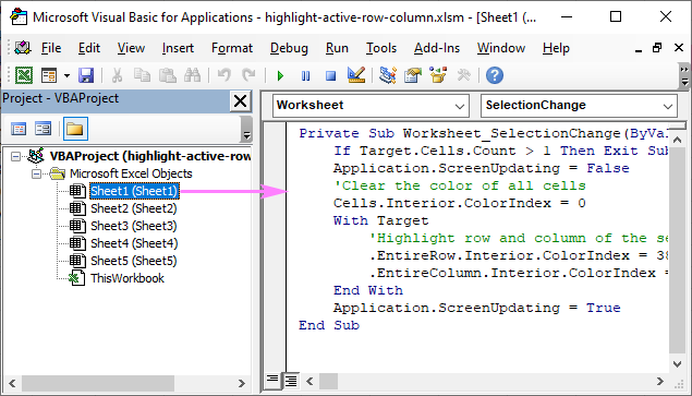
To have the code silently executed in the background of a specific worksheet, you need to insert it in the code window belonging to that worksheet, not in the normal module. To have it done, carry out these steps:
- In your workbook, press Alt + F11 to get to the VBA editor.
- In the Project Explorer on the left, you’ll see a list of all open workbooks and their worksheets. If you don’t see it, use the Ctrl + R shortcut to bring the Project Explorer window to view.
- Find the target workbook. In its Microsoft Excel Objects folder, double-click on the sheet in which you want to apply highlighting. In this example, it’s Sheet 1.
- In the Code window on the right, paste the above code.
- Save your file as Macro-Enabled Workbook (.xlsm).
Advantages: everything is done in the backend; no adjustments/customizations are needed on the user’s side; works in all Excel versions.
Drawbacks: there are two essential downsides that make this technique inapplicable under certain circumstances:
- The code clears background colors of all cells in the worksheet. If you have any colored cells, do not use this solution because your custom formatting will be lost.
- Executing this code blocksthe undo functionality on the sheet, and you won’t be able to undo an erroneous action by pressing Ctrl + Z .
Highlight active row and column without VBA
The best you can get to highlight the selected row and/or column without VBA is Excel’s conditional formatting. To set it up, carry out these steps:
- Select your dataset in which the highlighting should be done.
- On the Home tab, in the Styles group, click New Rule.
- In the New Formatting Rule dialog box, choose Use a formula to determine which cells to format.
- In the Format values where this formula is true box, enter one of these formulas:
To highlight active row:
To highlight active column:
To highlight active row and column:
=OR(CELL(«row»)=ROW(), CELL(«col»)= COLUMN())
All the formulas make use of the CELL function to return the row/column number of the selected cell.
If you feel like you need more detailed instructions, please see How to create formula-based conditional formatting rule.
For this example, we opted for the OR formula to shade both the column and row in the same color. That takes less work and is suitable for most cases. 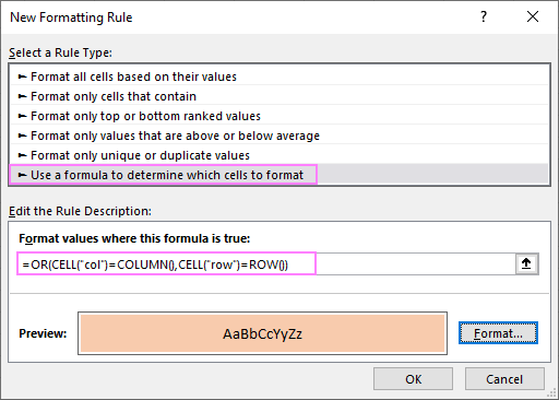
Unfortunately, this solution is not as nice as the VBA one because it requires recalculating the sheet manually (by pressing the F9 key). By default, Excel recalculates a worksheet only after entering new data or editing the existing one, but not when the selection changes. So, you select another cell — nothing happens. Press F9 — the sheet is refreshed, the formula is recalculated, and the highlighting is updated. 
To get the worksheet recalculated automatically whenever the SelectionChange event occurs, you can place this simple VBA code in the code module of your target sheet as explained in the previous example:
The code forces the selected range/cell to recalculate, which in turn forces the CELL function to update and the conditional formatting to reflect the change.
Advantages: unlike the previous method, this one does not impact the existing formatting you have applied manually.
Drawbacks: may worsen Excel’s performance.
- For the conditional formatting to work, you need to force Excel to recalculate the formula on every selection change (either manually with the F9 key or automatically with VBA). Forced recalculations may slow down your Excel. Since our code recalculates the selection rather than an entire sheet, a negative effect will most likely be noticeable only on really large and complex workbooks.
- Since the CELL function is available in Excel 2007 and higher, the method won’t work in earlier versions.
Highlight selected row and column using conditional formatting and VBA
In case the previous method slows down your workbook considerably, you can approach the task differently — instead of recalculating a worksheet on every user move, get the active row/column number with the help of VBA, and then serve that number to the ROW() or COLUMN() function by using conditional formatting formulas.
To accomplish this, here are the steps you need to follow:
- Add a new blank sheet to your workbook and name it Helper Sheet. The only purpose of this sheet is to store two numbers representing the row and column containing a selected cell, so you can safely hide the sheet at a later point.
- Insert the below VBA in the code window of the worksheet where you wish to implement highlighting. For the detailed instructions, please refer to our first example.
The above code places the coordinates of the active row and column to the sheet named «Helper Sheet». If you named your sheet differently in step 1, change the worksheet name in the code accordingly. The row number is written to A2 and the column number to B2.
And now, let’s cover the three main use cases in detail.
How to highlight active row
To highlight the row where your cursor is placed at the moment, set up a conditional formatting rule with this formula:
=ROW()=’Helper Sheet’!$A$2 
As the result, the user can clearly see which row is currently selected: 
How to highlight active column
To highlight the selected column, feed the column number to the COLUMN function using this formula:
=COLUMN()=’Helper Sheet’!$B$2 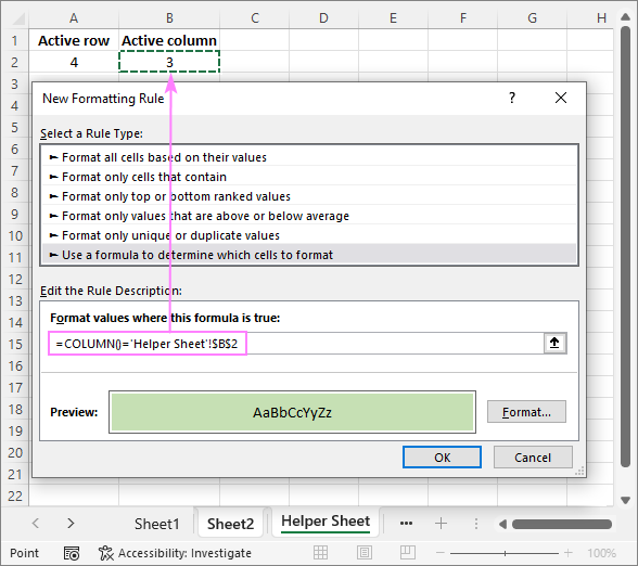
Now, a highlighted column lets you comfortably and effortlessly read vertical data focusing entirely on it. 
How to highlight active row and column
To get both the selected row and column automatically shaded in the same color, combine the ROW() and COLUMN() functions into one formula:
=OR(ROW()=’Helper Sheet’!$A$2, COLUMN()=’Helper Sheet’!$B$2) 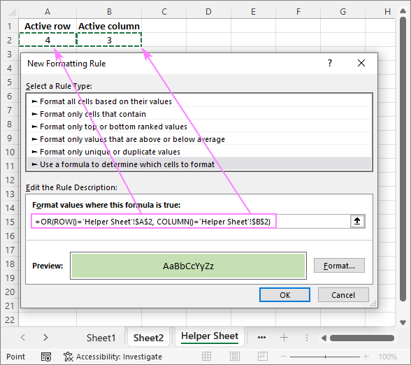
The relevant data is immediately brought into focus, so you can avoid misreading it. 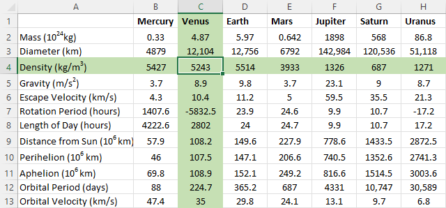
Advantages: optimized performance; works in all Excel versions
Drawbacks: the longest setup
That’s how to highlight the column and row of a selected cell in Excel. I thank you for reading and look forward to seeing you on our blog next week!
Источник