How do you freeze a row in excel

Freeze panes to lock rows and columns

To keep an area of a worksheet visible while you scroll to another area of the worksheet, go to the View tab, where you can Freeze Panes to lock specific rows and columns in place, or you can Split panes to create separate windows of the same worksheet.

Freeze rows or columns

Freeze the first column

• Select View > Freeze Panes > Freeze First Column.

            The faint line that appears between Column A and B shows that the first column is frozen.

Freeze the first two columns

1. Select the third column.

2. Select View > Freeze Panes > Freeze Panes.

Freeze columns and rows

1. Select the cell below the rows and to the right of the columns you want to keep visible when you scroll.

2. Select View > Freeze Panes > Freeze Panes.

Unfreeze rows or columns

• On the View tab > Window > Unfreeze Panes.

  

  Note: If you don’t see the View tab, it’s likely that you are using Excel Starter. Not all features are supported in Excel Starter.

Need more help?

You can always ask an expert in the Excel Tech Community or get support in the Answers community.

See Also

Freeze panes to lock the first row or column in Excel 2016 for Mac

Split panes to lock rows or columns in separate worksheet areas

Overview of formulas in Excel

How to avoid broken formulas

Find and correct errors in formulas

Keyboard shortcuts in Excel

Excel functions (alphabetical)

Excel functions (by category)

When you’re working with a lot of spreadsheet data on your laptop, keeping track of everything can be difficult. It’s one thing to compare one or two rows of information when dealing with a small subset of data, but when a dozen rows are involved, things get unwieldy. And we haven’t even started talking about columns yet. When your spreadsheets become unmanageable, there’s only one solution: freeze the rows and columns.

Freezing rows and columns in Excel makes navigating your spreadsheet much easier. When done correctly, the chosen panes are locked in place; this means those specific rows are always visible, no matter how far you scroll down. More often than not, you’ll only freeze a couple of rows or a column, but Excel doesn’t limit how many of either you can freeze, which can come in handy for larger sheets.

This how-to works with Microsoft Excel 2016 as well as later versions. However, the this method also works with Google Sheets, OpenOffice and LibreOffice. Ready to get to work? Here’s how to freeze rows and columns in Excel: 

• More: How to put Windows 10 into Safe Mode
• Here’s how to lock cells in Excel and how to recover a deleted or unsaved file in Excel
• This is how to use VLOOKUP in Excel and add additional rows above or below in Excel

How to freeze a row in Excel

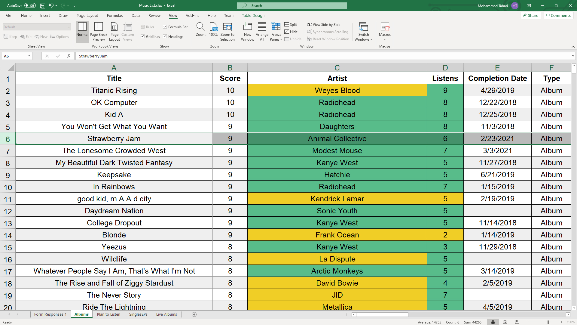
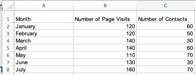
1. Select the row right below the row or rows you want to freeze. If you want to freeze columns, select the cell immediately to the right of the column you want to freeze. In this example, we want to freeze rows 1 to 5, so we’ve selected row 6.

2. Go to the View tab. This is located at the very top, inbetween «Review» and «Add-ins.»

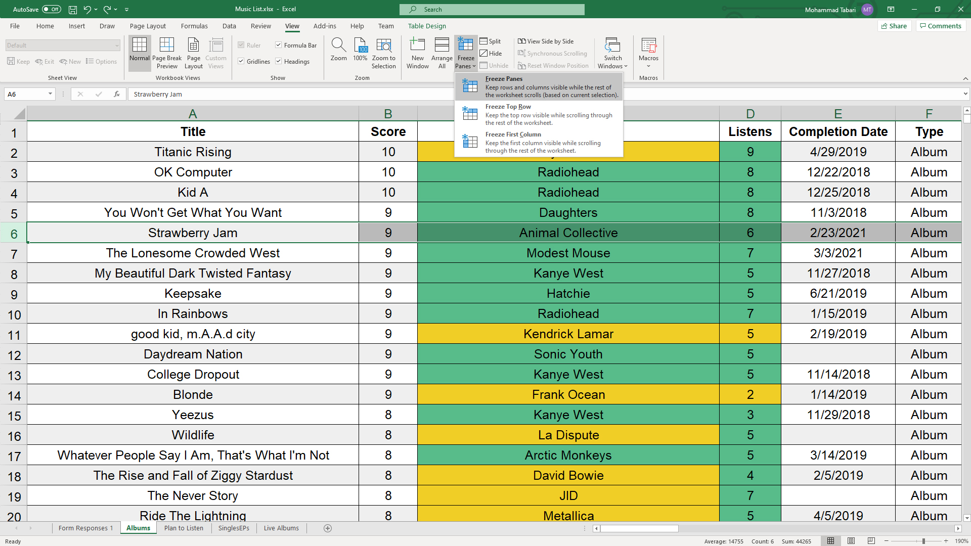
3. Select the Freeze Panes option and click «Freeze Panes.» This selection can be found in the same place where «New Window» and «Arrange All» are located.

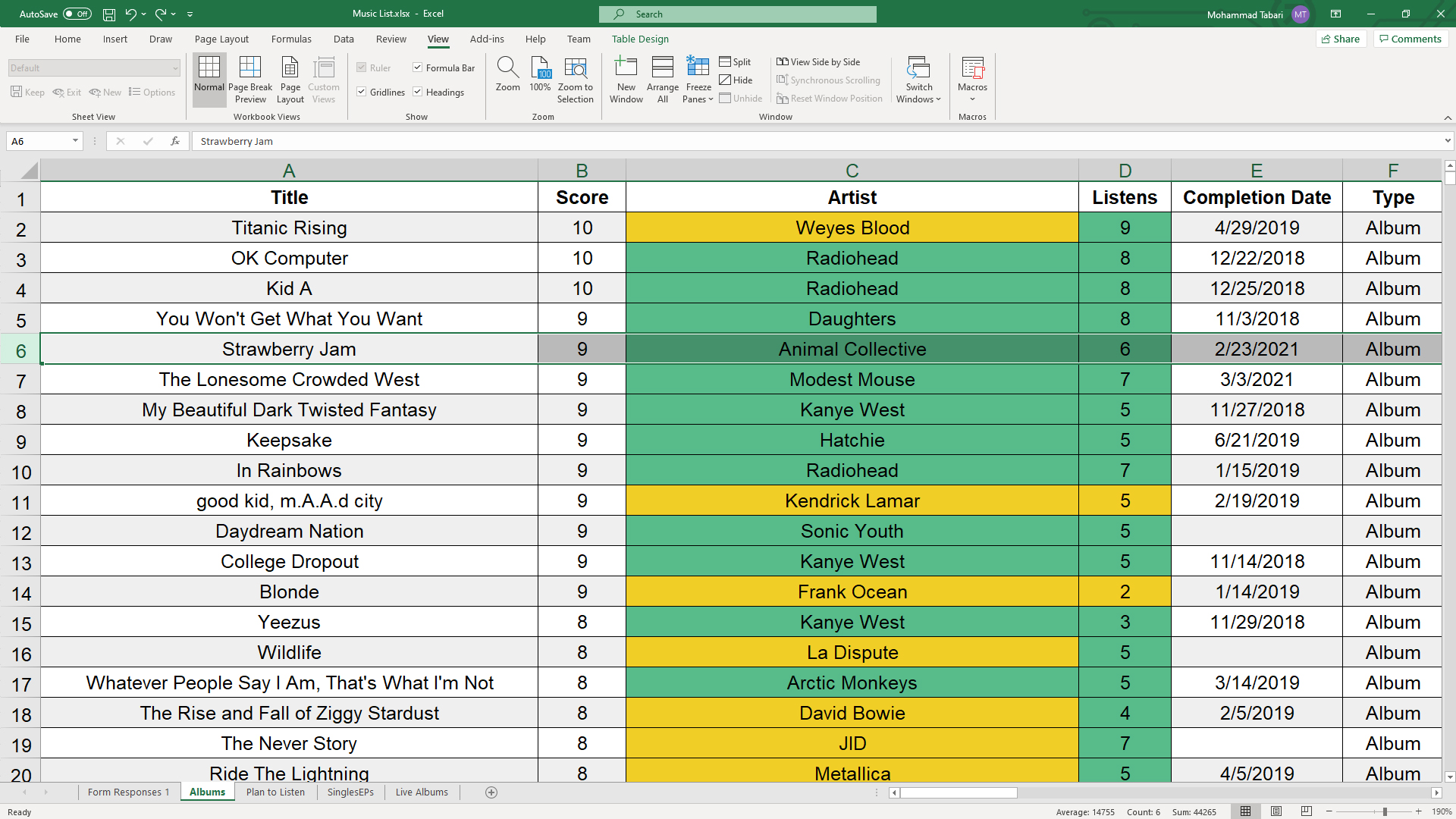
That’s all there is to it. As you can see in our example, the frozen rows will stay visible when you scroll down. You can tell where the rows were frozen by the green line dividing the frozen rows and the rows below them.

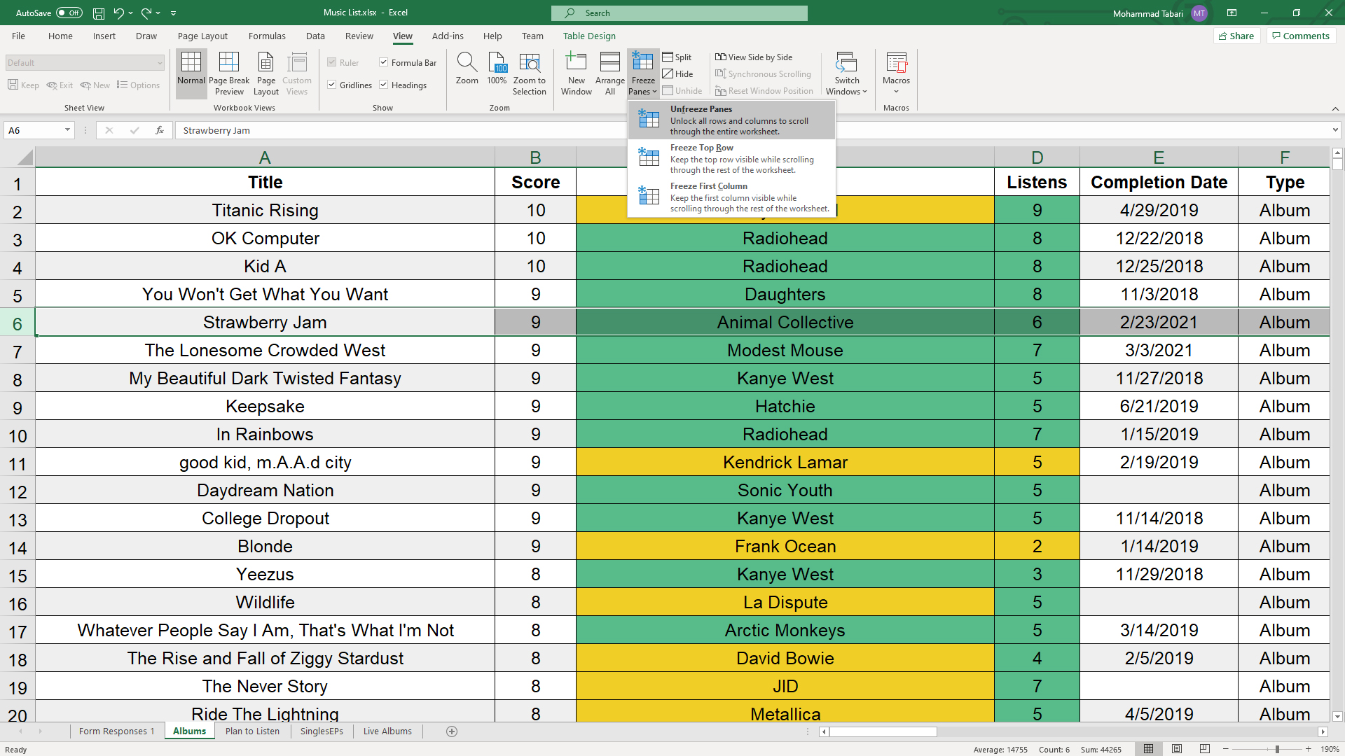
If you want to unfreeze the rows, go back to the Freeze Panes command and choose «Unfreeze Panes».

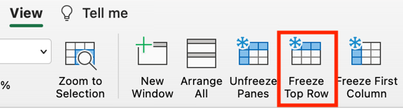
Note that under the Freeze Panes command, you can also choose «Freeze Top Row,» which will freeze the top row that’s visible (and any others above it) or «Freeze First Column,» which will keep the leftmost column visible when you scroll horizontally.

Besides allowing you to compare different rows in a long spreadsheet, the freeze panes feature lets you keep important information, such as table headings, always in view.

Need more Excel tricks? Check out our tutorials on How to Lock Cells in Excel and How to Use VLOOKUP in Excel.

Get instant access to breaking news, the hottest reviews, great deals and helpful tips.

Is this article up to date?

Without freezing rows or columns in your Excel spreadsheet, everything moves when you scroll through the page, as shown in the gif below.

This can be frustrating if you can’t always see key data markers that explain what data is what, like column headers or row titles.

As with many things on Excel, there are tricks that help you make your spreadsheets easier to read, like the freeze function. In this post, learn how to freeze rows and columns in Excel to ensure that, when you scroll around, you’ll always be able to view the key data points that matter most.

How to Freeze a Top Row in Excel

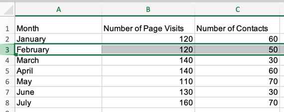
The image below is the sample data set I’ll use to run through the explanations in this piece.

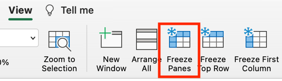
1. To freeze the top row in an Excel spreadsheet, navigate to the header toolbar and select View, as shown in the image below.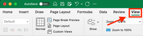

2. When the View menu options appear, Click Freeze Top Row, outlined in red in the image below.  

Once selected, everything in the top row of your Excel spreadsheet (row 1) will be frozen, and you can scroll up and down in your spreadsheet, but the top rows won’t move, as shown in the gif below.

How to Freeze a Specific Row in Excel

While excel has native functions for freezing the top row of a data set and the first column of a data set, there are additional steps to take to freeze other elements of your data set that aren’t those two things.

1. To freeze a specific row in Excel, select the row number immediately underneath the one you want frozen. For this example, I’m selecting row number three to freeze row number two.

2. After selecting your row, navigate to View in the header toolbar and select Freeze Panes.

Once selected, you’ll be able to scroll up and down through your spreadsheet and always see row two.

Note that using the Freeze Panes function to freeze rows also freezes every row above the row you initially selected. For example, in the gif below, I selected row five which also freeze rows four, three, two, and one.

How to Freeze the First Column in Excel

1. To freeze the first column of your Excel spreadsheet (column A), navigate to the Excel header toolbar, select View, and click Freeze First Column.

Once selected, you’ll be able to scroll side to side within your sheet, and the first column of your data set will always be visible, as shown in the image below.

How to Freeze a Specific Column in Excel

1. If you want to freeze a specific column in excel, select the column letter that is immediately next to the column you want frozen and click Freeze Panes in the View header menu.

Once selected, you can scroll side to side through your entire data set and continue to see those columns. In the gif below, I’ve frozen columns A and B.

Using the freeze function in Excel makes your spreadsheets easier to understand, as you can ensure that critical rows and columns are always visible as you scroll through your data.

Just assume you are school teacher and have around 90 students in a class which is divided into various sections. Now, you have to collate their marks in every subject in an excel.

If you are using a 15-inch laptop to do this, then as soon as you go to the 25^th row or later you lose the context of which column is for which subject. All of this happens because your header or first row is not fixed and keeps changing as you scroll down. But don’t worry we are here to help you out. 🙂

In this post we are going to help you on how to freeze rows or columns in excel. Freeing in excel will turn some cells (rows and / or columns) to be stagnant and these cells would not change if you move left or right or scroll up or down. There are various ways to freeze cells in excel.

We have listed all the methods below, if you do not want to go through the entire post then you may directly click on the type of excel freeze option you are looking for:

• Freeze First Row
• Freeze First Column
• Freeze Panes
  1. Freeze Multiple Rows
  2. Freeze Multiple Columns
  3. Freeze Rows & Columns at same time

Along with helping you on how to freeze in excel, we will also help you to unfreeze and troubleshooting issues that you might encounter:

• Unfreeze Panes
• Freeze panes versus Splitting Panes
• Freeze Pane is Disabled

Freeze First Row

This feature could be used to freeze a particular row or header that you would need to refer every time while working on excel. In this option only the top row will freeze.

• Open the sheet where in you want to freeze any row / header, as an example we would like to freeze the top row highlighted in yellow

• Now, navigate to the “View” tab in the Excel Ribbon as shown in above image
• Click on the “Freeze Panes” button

• Select “Freeze Top Row” option

• If you would like to freeze any other row, then scroll down and make that row appear as first in your sheet and then repeat Step 2 to 4.

That’s it. You are all set now. As seen in above image you can now scroll to any corner of the page and you would see that the top row remains intact all the time without any change.

Please note that this option works as long as first row in excel is the one that you really want to freeze. If you have scrolled in the middle of the sheet and Row 30 is appearing as first row, then this option would freeze Row 30 and not Row 1.

Additionally, if you are geek and would like to do it directly using a keyboard shortcut, then please press “Alt + W” followed by “F” and then “R”. Please note that this is not an in-built shortcut, rather it’s the same thing from keyboard as we do from mouse.

Freeze First Column

This feature could be used to freeze a particular column that you would need to refer while working on excel. In this option only the first column will freeze.

• Open the sheet where in you want to freeze the column, as an example we would like to freeze the column A – Product

• Now, navigate to the “View” tab in the Excel Ribbon as shown in above image
• Click on the “Freeze Panes” button

• Select “Freeze First Column” option

• If you would like to freeze any other column, then move right or left and make that column appear as first in your sheet and then repeat Step 2 to 4.

That’s it. You are all set now. As seen in above image you can now move to most right corner of the page and you would see that the first column sticks there. Please note that this option works as long as first column in excel is the one that you really want to freeze. If you have shifted right in the middle of the sheet and Column M is appearing as first row, then this option would freeze Column M and not Column A.

If you would like to do it directly using a keyboard shortcut, then please press “Alt + W” followed by “F” and then “C”. Please note that this is not an in-built shortcut, rather it’s the same thing from keyboard as we do from mouse.

Freeze Panes

This feature could be used to freeze multiple rows, columns or both at the same time. However, this could be done only for the consecutive rows or columns.

Freeze Panes – Multiple Rows

• Open the sheet where in you want to freeze the multiple rows, keep the first row on top and click after the last row till where you want to freeze, as an example we would like to freeze from Row 1 to Row 13 so we will click on Row 14

• Now, navigate to the “View” tab in the Excel Ribbon as shown in above image
• Click on the “Freeze Panes” button

• Select “Freeze Panes” option

That’s it. You are all set now. As seen in above image you can now scroll down and Row 1 to Row 13 will be kept intact without any changes. You can select the range of rows from middle as well like – Row 13 to Row 30, however to do so you will have to ensure that you scroll up and keep Row 13 as your first row in the sheet and repeat the steps listed above. However, be careful as doing so some of your rows (i.e. the ones before Row 13) will be hidden.

Freeze Panes – Multiple Columns

• Open the sheet where in you want to freeze the multiple columns, keep the first column to the left and click next to the last column till where you want to freeze, as an example we would like to freeze from Column A to E, so we will click on Column F

• Now, navigate to the “View” tab in the Excel Ribbon as shown in above image
• Click on the “Freeze Panes” button

• Select “Freeze Panes” option

That’s it. You are all set now. As seen in above image you can now move towards right and Column A to E will be kept intact without any changes. You can select the range of columns from middle as well like – Column F to Column L, however to do so you will have to ensure that you move to the left and keep Column F as your first column in the sheet and repeat the steps listed above. However, be careful as doing so some of your columns (i.e. the ones before Column E) will be hidden.

Freeze Panes – Multiple Rows and Columns both

If you have followed the post till now, then you would have already figured out how this has to be done. Yes, you are right we are going to club both the above listed approaches here. Follow us below:

• Open the sheet where in you want to freeze the multiple rows and columns, keep the first row on top and first column to the left then click next to the cell of the last column and row till where you want to freeze, as an example we would like to freeze from Row 1 to 13 and Column A to E, so we will click on Cell F14

• Now, navigate to the “View” tab in the Excel Ribbon as shown in above image
• Click on the “Freeze Panes” button

• Select “Freeze Panes” option

That’s it. You are all set now. As seen in above image you can now scroll down and Row 1 to 13 will remain intact and likewise you can move towards right and Column A to E will be kept intact without any changes. You can select the range of columns from middle as well like – Row 17 to 27 and Column F to L, however to do so you will have to ensure that you scroll up and keep Row 17 as your first row and keep Column F as your first column in the sheet and repeat the steps listed above. Be careful here as rows before Row 17 and columns before column F will be hidden.

Unfreeze Panes:

If you have frozen the wrong rows and columns, then you could easily undo it by using “Unfreeze Panes” option. This would remove all the frozen rows and or columns in your excel. This will also work if you have received the sheet from someone else and you are not able to see all the rows and columns despite of removing all filters and unhiding rows columns. To unfreeze panes –

• Open the sheet wherein you want to unfreeze rows and or columns
• Now, navigate to the “View” tab in the Excel Ribbon
• Click on the “Freeze Panes” button

• Select “Unfreeze Panes” option as shown above

With this all the rows and or columns would unfreeze, as shown in above image. Please note that you would not see the “Unfreeze Panes” option if there are not any frozen rows columns. This option would be available only and only when there is some row and or column frozen already.

If you would like to unfreeze panes it directly using a keyboard shortcut, then please press “Alt + W” followed by “F” and then again “F”. Please note that this is not an in-built shortcut, rather it’s the same thing from keyboard as we do from mouse.

Freeze panes versus Splitting Panes:

Excel also provides you an excellent option to Split Panes which divides the window into different panes that each pane scrolls separately. This option is present in Excel Ribbon, View tab next to Freeze Option.

So as visible in the above image after using split option the content of same sheet is visible in 4 separate panes and all panes have their different scroll options.

We personally trust and use Freeze option much than Split, as Freeze allows you to limit the data movement by freezing it rather than adding multiple views of same data wherein you easily get distracted and confused while data entry.

Is Freeze Pane option disabled?

If you have come across a case wherein the Freeze Pane option is disabled in your sheet, then it must be due to one of the following reasons:

• The most common reason of Freeze Panes option disablement is that your sheet must have been opened in “Page Layout” mode (as shown in below image)

In order to correct it simply navigate to “View Tab” in the excel ribbon and select “Normal” or “Page Break” view.

• The “Freeze Panes” option could also be disabled if you excel has been protected for windows. You would need to unprotect it to enable the freeze option.

So, this was all about how to freeze rows and columns in Excel. Hope you enjoyed our tutorial. Please feel free to share your feedback and queries. Keep Exceling 🙂