
Change the format of a cell
You can apply formatting to an entire cell and to the data inside a cell—or a group of cells. One way to think of this is the cells are the frame of a picture and the picture inside the frame is the data.

Formal Cells
-
Select the cells.
-
Go to the ribbon to select changes as Bold, Font Color, or Font Size.
Apply Excel Styles
-
Select the cells.
-
Select Home > Cell Style and select a style.
Modify an Excel Style
-
Select the cells with the Excel Style.
-
Right-click the applied style in Home > Cell Styles.
-
Select Modify > Format to change what you want.
Need more help?
You can always ask an expert in the Excel Tech Community or get support in the Answers community.
See Also
Format text in cells
Format numbers
Format a date the way you want
Need more help?
![]()
Download Article
![]()
Download Article
Knowing how to format your spreadsheet in Excel, the cells in particular, can really help you improve not just the aesthetic perspective of your document, but also its effectiveness in providing relevant information to the viewers of the files. Each cell in Microsoft Excel can be modified and formatted to follow your specific preferences.
-

1
Open your Microsoft Excel. Click the “Start” button on the lower-left corner of your screen and select “All Programs” from the menu. Inside, you’ll find the “Microsoft Office” folder where Excel is listed. Click on Excel.
-
2
Select the specific cell or group of cells that you want to format. Highlight it using your mouse cursor.
Advertisement
-
3
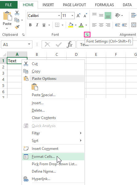
Open the Format Cells window. Right-click on the cells you’ve selected and select “Format Cells” from the pop up menu to access the “Format Cells” window.
-
4
Set the desired formatting options you want for the cell. There are six formatting options that you can use to customize a cell or group of cells:
- Number – Defines the format of numerical data entered on the cells such as dates, currency, time, percentage, fraction and more.
- Alignment – Sets how the data will be visually aligned inside each cells (left, right or centered).
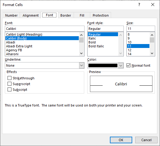
- Font – Sets all the options related to text fonts such as styles, sizes and colors.
- Border – Improves the visual appearance of each cell by adding definite lines (borders) around a cell or group of cells.
- Fill – Sets the background color and pattern formats of each cell on the spreadsheet.
- Protection – Adds security to cells and data contained inside it by hiding or locking the selected cells or group of cells.
-
5
Save. Click on the “OK” button at the lower right corner of the “Format Cells” window to save any changes you’ve made and apply the formats you’ve set to the selected cells.


Advertisement
Ask a Question
200 characters left
Include your email address to get a message when this question is answered.
Submit
Advertisement
-
Avoid using formats that are visually irritating such as fill colors that don’t compliment the colors of the fonts, or artistic font styles that are not appropriate for formal documents like the spreadsheet.
-
You can use this method to format cells of new files or existing spreadsheet documents you currently have.
-
When formatting cells in Excel, do it in groups (either by rows or columns) so that your spreadsheet will have a clean and uniform appearance.
Thanks for submitting a tip for review!
Advertisement
About This Article
Article SummaryX
To format a cell in Microsoft Excel, start by highlighting the specific cell you want to format. Then, right-click on the cell and click on «Format Cells.» Choose whatever formatting you want for the cell from the different options, then click «Okay.» That’s all there is to it! For a step-by-step walkthrough with pictures, check out the full article below!
Did this summary help you?
Thanks to all authors for creating a page that has been read 72,532 times.
Is this article up to date?
When you fill out Excel worksheets with data, no one will succeed at once, everything is beautiful and correctly filled at the first attempt.
In the process of working with the program, you always need something: modify, edit, delete, copy or move. If the entered incorrect values in a cell, naturally, we want to correct or delete ones. But even such simple task can sometimes create difficulties.
How to set the cell format in Excel?
The contents of each Excel cell consist of three elements:
- The meaning: text, numbers, dates and times, logical content, functions and formulas.
- The formats: the type and color of the borders, the type and color of the fill, the way the values are displayed.
- Comments.
All these three elements are completely independent of each other. You can specify the format of the cell and do not write anything to it, or add a note in an empty and not formatted cell.
How to change the format of cells in Excel?
To change the format of the cells, you should call the corresponding dialog box with the CTRL + 1 (or CTRL + SHIFT + F) key or from the context menu after you right-click the «Cell Format» option.
There are 6 tabs in this dialog box:
- A number. Here you specify the way the numeric values are displayed.
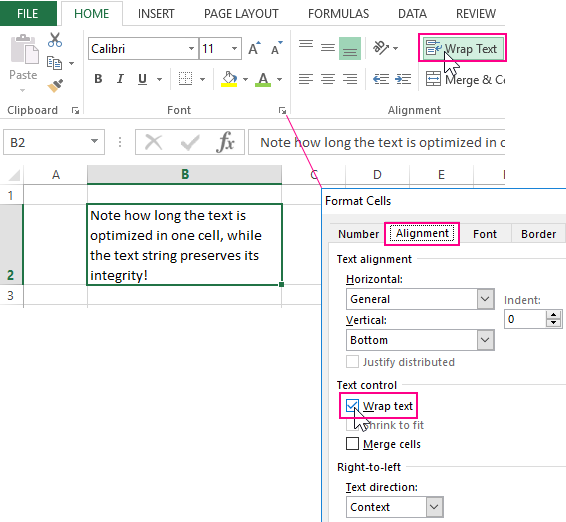
- The alignment. On this tab you can control the position of the text. And the text can be displayed vertically or diagonally from any angle. Also pay attention to the «Display» section. Very often, the function «Wrap Text» is used.
- Font. The specify the style design of fonts, the size and color of the text, plus the modes of modifications.
- The border. Here you define the styles and colors of the borders. The design of all tables is better done right here.
- The fill. The name of the bookmark speaks for itself. Available for formatting colors, patterns and methods of filling (for example, a gradient with a different direction of strokes).
- The protection. Here, the cell protection settings are set, that are activated only after the protection of the whole sheet.
If you did not get the desired result on the first attempt, call this dialog again to fix the cell format in Excel.
What formatting is applicable to cells in Excel?
Each cell always has some format. If there were no changes, then this is the «General» format. It is also a standard Excel format, in which:
- the numbers are aligned on the right side;
- the text is aligned on the left side;
- the font Calibri with the height of 11 points;
- the cell has no borders and background fill.
The Format Removal – is the changing to the standard «General» format (without borders and fills).
It is worth noting that the format of cells, unlike values, can not be deleted with the DELETE key.
To delete the format of cells, select ones and use the «Clear Formats» tool, which is located on the «HOME» tab in the «Editing» section.
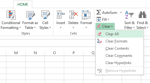
If you want to clear not only the format, but also the values, then select the «Clear All» option from the drop-down list of the tool (eraser).
As you can see, the eraser tool is functionally flexible and allows us to make a choice of what to delete in the cells:
- the content (same as the DELETE key);
- the formats;
- notes;
- the hyperlinks.
The option «Clear all» combines all these functions.
The deleting notes
Note, as well as formats, are not deleted from the cell by pressing the DELETE key. You can delete notes in two ways:
- The eraser tool: the option «Clear notes».
- Click on the cell with the note with the right mouse button, and from the appeared context menu select the option «Delete note».
The notation. The second way is more convenient. If you delete several notes at the same time, you must first select all of its cells.
Definition of Format Cells
A format in excel can be defined as the change of appearance of the data in the cell the way it is, without changing the actual data or numbers in the cells. That means the data in the cell remains the same, but we will change the way it looks.
Different Formats in Excel
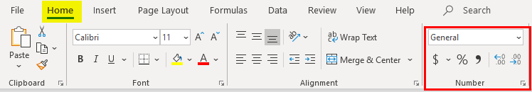
We have multiple formats in Excel to use. To see the available formats in excel, click on the “Home” menu on the top left corner.
General Format
In General format, there is no specific format; whatever you input, it will appear in the same way; it may be a number or text or symbol. After clicking on the HOME menu, go to the “NUMBER” segment, where you can find a drop of formats.
Click on the drop-down where you see the “General” option.
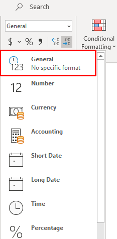
We will discuss each of these formats one by one with related examples.
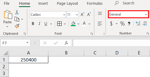
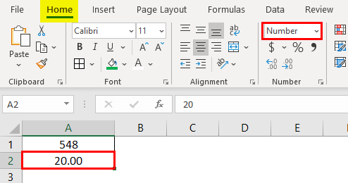
1. Number Format
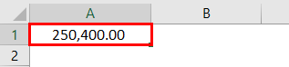
This format converts the data to a number format. When we input the data initially, it will be in General format; after converting to Number format only, it will appear as number format. Observe the below screenshot for the number in General format.
Now choose the format “Number” from the drop-down list and see how the appearance of cell A1 changes.
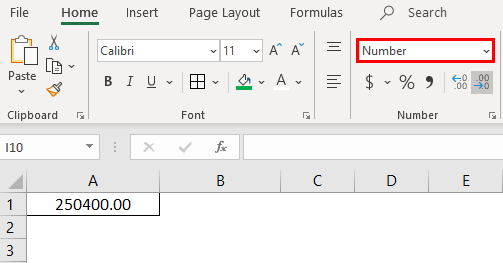
That is a difference between the General and Number format. If you want further customizations to your number format, select the cell that you want to do customization and right-click the below menu will come.
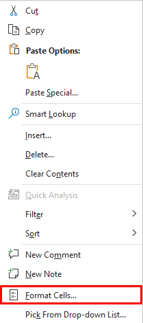
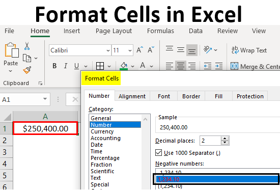
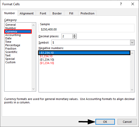
Choose the “Format Cells“ option then you will get the below window.
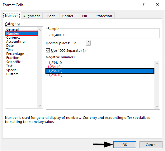
Choose “Number” under the “Category” option then you will get the customizations for the Number format. Choose the number of decimals you want to display. Tick the checkbox “Use 1000 separator” for separation of 1000’s with a comma (,).
Choose the negative number format whether you want to display with a negative symbol, brackets, red colour, nd red col, etc.
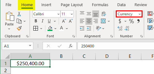
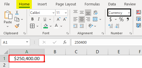
2. Currency Format
Currency format helps to convert the data to a currency format. We have an option to choose the type of currency as per our requirement. Select the cell which you want to convert to Currency format and choose the “Currency” option from the drop-down.
Currently, it is in Dollar currency. We can change by clicking on the drop-down of “$” and choose your required currency.
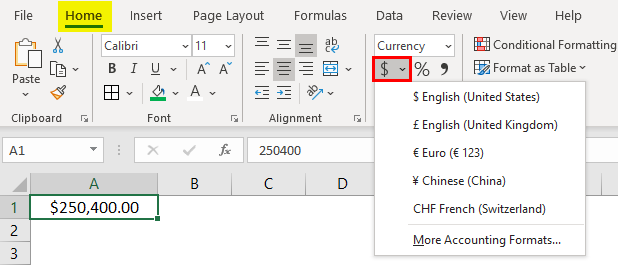
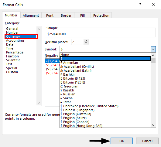
In the drop-down, we have few currencies; if you want the other currencies, click on the option “More Accounting formats”, which will display a pop-up menu as below.
Click on the drop-down “Symbol” and choose the required currency format.
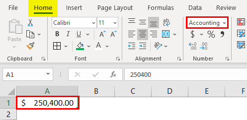
3. Accounting Format
As you all know, accounting numbers are all related to money; hence whenever we convert any number to accounting format, it will add a currency symbol to that. The difference between currency and accounting is currency symbol alignment. Below are the screenshots for reference.
4. Accounting Alignment
5. Currency Alignment
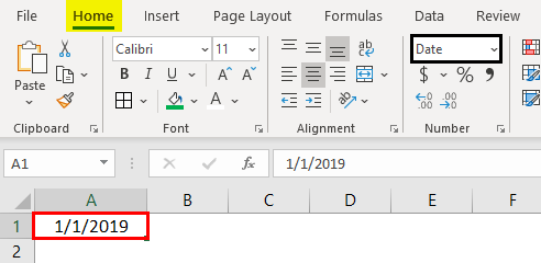
6. Short Date Format
A date can represent in a short format and long format. When you want to represent your date in a short format, use the short date format. E.g., 1/1/2019.
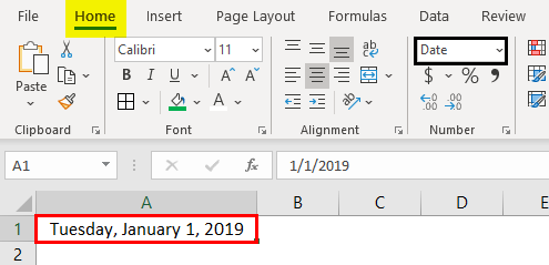
7. Long Date Format
The long date is used to represent our date in an expandable format like the below screenshot.
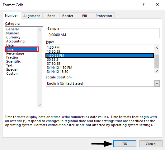
We see the short date format and long date format have multiple formats to represent our dates. Right-click and select “Format Cells” as to how we did before for “numbers”, then we will get the window to select the required formats.
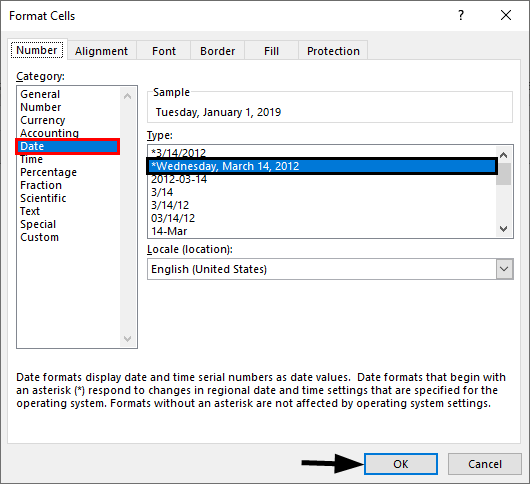
You can choose the location from the “Locale” drop-down menu.
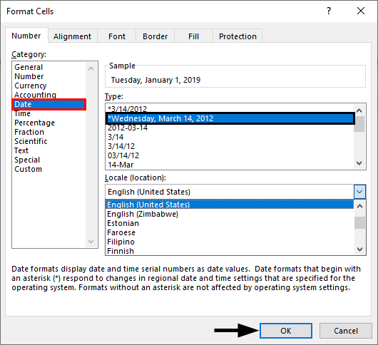
Choose the date format under the “Type” menu.
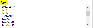
We can represent our date in any of the formats from the available formats.
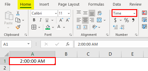
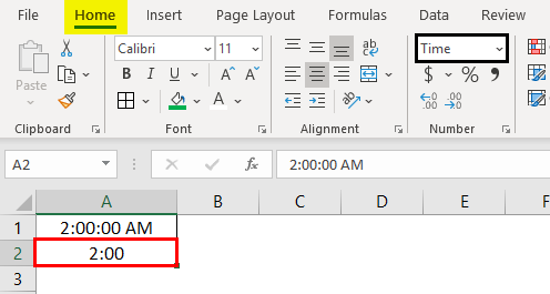
8. Time Format
This format is used to represent the time. If you input time without converting the cell into time format, it will show normally, but if you convert the cell into time format and input, it will clearly represent the time. Find the below screenshot for the differences.
If you still want to change the time format, then change in the format cells menu as shown below.
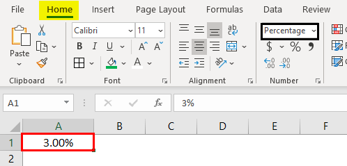
9. Percentage Format
Suppose you want to represent the number percentage use this format. Input any number in the cell and select that cell and choose the percentage format then the number will convert into a percentage.
10. Fraction Format
When we input the fraction numbers like 1/5, we should convert the cells into Fraction format. If we input the same 1/5 in a normal cell, it will show as a date.
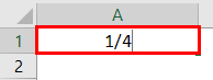
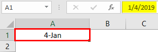

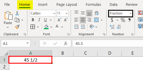
This is how the fraction format works.
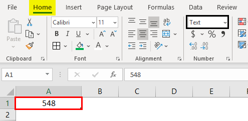
11. Text Format
When you input the number and convert it to text format, the number will align to the left side. It will consider as text as only, not the number.
12. Scientific Format
When you input a number 10000 (Ten thousand) and convert it into a scientific format, it will display as 1E+04, here E means exponent and 04 represents the number of zeros. If we input the number 0.0003, it will display as 3E-04. Try different numbers in excel format and check you will get a better idea to understand this better.
13. Other Formats
Apart from the explained formats, we have other formats like Alignment, Font, Border, Fill, and Protection.
Most of them are self-explanatory; hence I am leaving and explaining protection alone. When you want to lock any cells in the spreadsheet, use this option. But this lock will enable only when you protect the sheet.
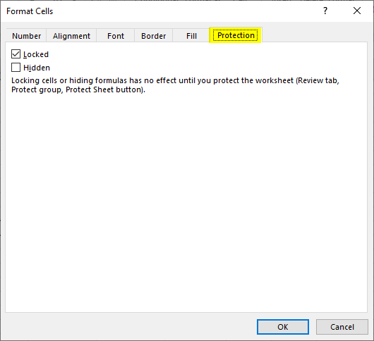
You can hide and lock the cells on the same screen; Excel has provided instructions on when it will affect.
Things to Remember About Format Cells in Excel
- One can apply formats by right-clicking and selecting the format cells or from the drop-down as explained initially. The impact of them is the same; however, you will have multiple options when you right-click.
- When you want to apply a format to another cell, use format painter, select the cell, click on formatted painters, and choose the cell you want to apply.
- Use the option “Custom” when you want to create your own formats as per requirement.
Recommended Articles
This is a guide to Format Cells in Excel. Here we discuss how to format cells in excel along with practical examples and a downloadable excel template. You can also go through our other suggested articles to learn more–
- Excel Conditional Formatting for Dates
- Auto Format in Excel
- Formatting Text in Excel
- Excel Format Phone Numbers
What Is Excel Format Cells?
Formatting cells in Excel is one of the key options used to format the data. We can format data in different formats, such as time, date, currency, font, etc.,
For example, using format cells in excel, we can format time. If the value is 1800 hrs and we want to format it based on hh:mm AM/PM format, we can use the format cells option. As soon as we click format, the 1800 hrs will be formatted into 06:00 PM.
Table of contents
- What Is Excel Format Cells?
- How To Format Cells In Excel?
- Examples
- Important Things To Remember
- Frequently Asked Questions (FAQs)
- Recommended Articles
- Format cells in excel are used to format the data in the worksheet to present well and to save time.
- The tabs available in the Format cells option in excel are number, alignment, font, border, fill, and protection.
- Using the Number tab, we can format values such as date, currency, time, percentage, fraction, scientific notation, accounting number, etc., in excel.
- The shortcut keys to format date (in dd-mm-yy format) are Ctrl+Shift+#.
- Similarly, the shortcut keys to format time in hh:mm AM/PM format is [email protected]
How To Format Cells In Excel?
Formatting cells in excel is really simple. Let us have a look at the following examples to learn how to use format cells in excel.
You can download this Format Cell Excel Template here – Format Cell Excel Template
Examples
Example #1 – Format Date Cell
Excel stores date and time as serial numbers. We need to apply an appropriate format to the cell to see the date and time correctly.
For example, look at the below data.

It looks like a serial number to us, but we get date values when applying date format in excel to these serial numbers.
The date has a wide variety of formats. Below is a list of formats we can apply to dates.

We can apply any formatting codes to see the date, as shown above in the respective format.
- To apply the date format, we must first select the range of cells and press Ctrl + 1 to open the format window. Then, under Custom, we must apply the code as we want to see the date.
Format Cells Shortcut Key
![]()

We get the following result.

Example #2 – Format Time Cell
As we said, the date and time are stored as serial numbers in Excel. Now, it is time to see the TIME formatting in excel. For example, look at the numbers below.

The TIME values are varied from 0 to less than 0.99999, so let us apply the time format to see the time. Below are the time format codes we can generally use:
“h:mm:ss”
To apply the time format, we must follow the same steps:

So, we get the following result.

So, the number “0.70192” equals the time of 16:50:46.
If we do not want to see the time in the 24-hour format, we need to apply the time formatting code like the one below.

Now, we will get the result as shown in the below image.

Now, our time is shown as 04:50:46 PM instead of 16:50:46.
Example #3 – Format Date And Time Together
The date and time are together in Excel. We can format both the date and time together in Excel. For example, look at the below data.

Let us apply the date and time format to these cells to see the results. The formatting code is dd-mmm-yyyy hh:mm:ss AM/PM.

We get the following result.

Let us analyze this briefly now.
The first value we had was 43689.6675 for this, we have applied the date and time format as dd-mm-yyyy hh:mm:ss AM/PM, so the result is 12-Aug-2019 04:01:12 PM.
43689 represents data in this number, and the decimal value 0.6675021991 represents time.
Example #4 – Positive And Negative Values
When dealing with numbers, positive and negative values are part of it. To differentiate between these two values by showing them with different colors is the general rule everybody follows. For example, look at the below data.

To apply a number format to these numbers and show negative red values, below is the code.

“#,###;[Red]-#,###”
If we apply this formatting code, we can see the above numbers.

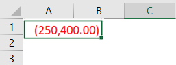
Similarly, showing negative numbers in brackets is also in practice. For example, to show the negative numbers in the bracket and red color, below is the code.
“#,###;[Red](-#,###)”

We get the following result.

Example #5 – Add Suffix Words To Numbers
If we want to add suffix words along with numbers and still be able to do calculations, it is great.
If we show a person’s weight, adding the suffix word KG will add more value to the numbers. Below is the person’s weight in KG.

To show this data with the suffix word KG, apply the below formatting code.
### ” KG”

After applying the code, the weight column looks like as shown below.

Example #6 – Using Format Painter
Format Painter Excel, we can apply one cell format to another. For example, look at the below image.

The date format is DD-MM-YYYY, and the remaining cells are not formatted for the first cell. But, we can apply the format of the first cell to the remaining cells by using a format painter.
We must select the first cell, then go to the Home tab and click on Format Painter.

Now, we must click on the next cell to apply the formatting.

Now again, select the cell and apply the formatting, but this is not the smart way of using a format painter. Instead, double-click on Format Painter by selecting the cell. Once we double-click, we can apply the format to any number of cells, applying all at once.

Important Things To Remember
- The format option is used to format the data in different formats.
- We can format the date and time together.
- The Excel Format Painter is the tool used to copy one cell format to another.
Frequently Asked Questions (FAQs)
1. What are format cells in excel?
Format cells is an option used to format the values used in excel.
We can use the format cells option by clicking on
Home → Cells group → Format drop-down option → Format Cells
2. How to format data in excel?
We can format the date with simple steps;
Consider the following example. The date of birth of 3 people is in 3 different formats. Now, let us learn how to format the date such that cell range B2:B4 are in the same format.

The steps used to format date are:
• Step 1: Select cell B2.
• Step 2: Select Home → Cells group → Format drop-down option → Format Cells
• Step 3: The Format Cells tab pops up.

• Step 4: Click Date from the Category under Number tab.

• Step 5: We can select the desired option. In our example, let us select the 4th option.
As we click OK¸ we can see that the value in cell B2 is formatted.

Similarly, we can format cells in excel.
3. What are the shortcut keys to format cells in excel?
The following are some useful shortcut keys to format cells in excel:
• Ctrl+Shift+~ – General Format
• Ctrl+Shift+# – Format Date
• [email protected] – Format Time
Recommended Articles
This article is a guide to Format cells in Excel. Here, we discuss the top 6 tips to format cells, including date, time, date and time together, format painter, etc., examples, and a downloadable Excel template. You may also look at these useful functions in Excel: –
- Shortcut Key to Start New Line in Excel Cell
- Export Excel into PDF File
- How to Format Phone Numbers in Excel?
- Accounting Number Excel Format