
Use AutoFilter or built-in comparison operators like «greater than» and “top 10” in Excel to show the data you want and hide the rest. Once you filter data in a range of cells or table, you can either reapply a filter to get up-to-date results, or clear a filter to redisplay all of the data.
Use filters to temporarily hide some of the data in a table, so you can focus on the data you want to see.

Filter a range of data
-
Select any cell within the range.
-
Select Data > Filter.

-
Select the column header arrow
. -
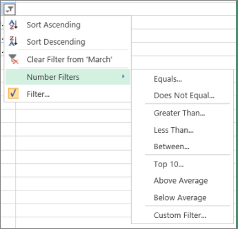
Select Text Filters or Number Filters, and then select a comparison, like Between.
-
Enter the filter criteria and select OK.
Filter data in a table
When you put your data in a table, filter controls are automatically added to the table headers.

-
Select the column header arrow
for the column you want to filter. -
Uncheck (Select All) and select the boxes you want to show.
-
Click OK.
The column header arrow
changes to a Filter icon. Select this icon to change or clear the filter.
Related Topics
Excel Training: Filter data in a table
Guidelines and examples for sorting and filtering data by color
Filter data in a PivotTable
Filter by using advanced criteria
Remove a filter
Filtered data displays only the rows that meet criteria that you specify and hides rows that you do not want displayed. After you filter data, you can copy, find, edit, format, chart, and print the subset of filtered data without rearranging or moving it.
You can also filter by more than one column. Filters are additive, which means that each additional filter is based on the current filter and further reduces the subset of data.
Note: When you use the Find dialog box to search filtered data, only the data that is displayed is searched; data that is not displayed is not searched. To search all the data, clear all filters.
The two types of filters
Using AutoFilter, you can create two types of filters: by a list value or by criteria. Each of these filter types is mutually exclusive for each range of cells or column table. For example, you can filter by a list of numbers, or a criteria, but not by both; you can filter by icon or by a custom filter, but not by both.
Reapplying a filter
To determine if a filter is applied, note the icon in the column heading:
-
A drop-down arrow
means that filtering is enabled but not applied.When you hover over the heading of a column with filtering enabled but not applied, a screen tip displays «(Showing All)».
-
A Filter button
means that a filter is applied.When you hover over the heading of a filtered column, a screen tip displays the filter applied to that column, such as «Equals a red cell color» or «Larger than 150».
When you reapply a filter, different results appear for the following reasons:
-
Data has been added, modified, or deleted to the range of cells or table column.
-
Values returned by a formula have changed and the worksheet has been recalculated.
Do not mix data types
For best results, do not mix data types, such as text and number, or number and date in the same column, because only one type of filter command is available for each column. If there is a mix of data types, the command that is displayed is the data type that occurs the most. For example, if the column contains three values stored as number and four as text, the Text Filters command is displayed .
Filter data in a table
When you put your data in a table, filtering controls are added to the table headers automatically.
-
Select the data you want to filter. On the Home tab, click Format as Table, and then pick Format as Table.
-
In the Create Table dialog box, you can choose whether your table has headers.
-
Select My table has headers to turn the top row of your data into table headers. The data in this row won’t be filtered.
-
Don’t select the check box if you want Excel for the web to add placeholder headers (that you can rename) above your table data.
-
-
Click OK.
-
To apply a filter, click the arrow in the column header, and pick a filter option.
Filter a range of data
If you don’t want to format your data as a table, you can also apply filters to a range of data.
-
Select the data you want to filter. For best results, the columns should have headings.
-
On the Data tab, choose Filter.
Filtering options for tables or ranges
You can either apply a general Filter option or a custom filter specific to the data type. For example, when filtering numbers, you’ll see Number Filters, for dates you’ll see Date Filters, and for text you’ll see Text Filters. The general filter option lets you select the data you want to see from a list of existing data like this:
Number Filters lets you apply a custom filter:
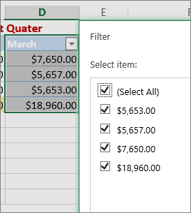
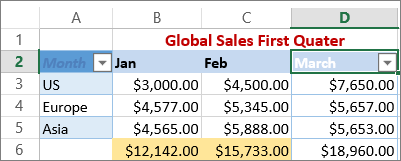
In this example, if you want to see the regions that had sales below $6,000 in March, you can apply a custom filter:
Here’s how:
-
Click the filter arrow next to March > Number Filters > Less Than and enter 6000.
-
Click OK.
Excel for the web applies the filter and shows only the regions with sales below $6000.
You can apply custom Date Filters and Text Filters in a similar manner.
To clear a filter from a column
-
Click the Filter
button next to the column heading, and then click Clear Filter from <«Column Name»>.
To remove all the filters from a table or range
-
Select any cell inside your table or range and, on the Data tab, click the Filter button.
This will remove the filters from all the columns in your table or range and show all your data.
-
Click a cell in the range or table that you want to filter.
-
On the Data tab, click Filter.
-
Click the arrow
in the column that contains the content that you want to filter. -
Under Filter, click Choose One, and then enter your filter criteria.
Notes:
-
You can apply filters to only one range of cells on a sheet at a time.
-
When you apply a filter to a column, the only filters available for other columns are the values visible in the currently filtered range.
-
Only the first 10,000 unique entries in a list appear in the filter window.
-
Click a cell in the range or table that you want to filter.
-
On the Data tab, click Filter.
-
Click the arrow
in the column that contains the content that you want to filter. -
Under Filter, click Choose One, and then enter your filter criteria.
-
In the box next to the pop-up menu, enter the number that you want to use.
-
Depending on your choice, you may be offered additional criteria to select:
Notes:
-
You can apply filters to only one range of cells on a sheet at a time.
-
When you apply a filter to a column, the only filters available for other columns are the values visible in the currently filtered range.
-
Only the first 10,000 unique entries in a list appear in the filter window.
-
Instead of filtering, you can use conditional formatting to make the top or bottom numbers stand out clearly in your data.
You can quickly filter data based on visual criteria, such as font color, cell color, or icon sets. And you can filter whether you have formatted cells, applied cell styles, or used conditional formatting.
-
In a range of cells or a table column, click a cell that contains the cell color, font color, or icon that you want to filter by.
-
On the Data tab, click Filter .
-
Click the arrow
in the column that contains the content that you want to filter. -
Under Filter, in the By color pop-up menu, select Cell Color, Font Color, or Cell Icon, and then click a color.
This option is available only if the column that you want to filter contains a blank cell.
-
Click a cell in the range or table that you want to filter.
-
On the Data toolbar, click Filter.
-
Click the arrow
in the column that contains the content that you want to filter. -
In the (Select All) area, scroll down and select the (Blanks) check box.
Notes:
-
You can apply filters to only one range of cells on a sheet at a time.
-
When you apply a filter to a column, the only filters available for other columns are the values visible in the currently filtered range.
-
Only the first 10,000 unique entries in a list appear in the filter window.
-
-
Click a cell in the range or table that you want to filter.
-
On the Data tab, click Filter .
-
Click the arrow
in the column that contains the content that you want to filter. -
Under Filter, click Choose One, and then in the pop-up menu, do one of the following:
To filter the range for
Click
Rows that contain specific text
Contains or Equals.
Rows that do not contain specific text
Does Not Contain or Does Not Equal.
-
In the box next to the pop-up menu, enter the text that you want to use.
-
Depending on your choice, you may be offered additional criteria to select:
To
Click
Filter the table column or selection so that both criteria must be true
And.
Filter the table column or selection so that either or both criteria can be true
Or.
-
Click a cell in the range or table that you want to filter.
-
On the Data toolbar, click Filter .
-
Click the arrow
in the column that contains the content that you want to filter. -
Under Filter, click Choose One, and then in the pop-up menu, do one of the following:
To filter for
Click
The beginning of a line of text
Begins With.
The end of a line of text
Ends With.
Cells that contain text but do not begin with letters
Does Not Begin With.
Cells that contain text but do not end with letters
Does Not End With.
-
In the box next to the pop-up menu, enter the text that you want to use.
-
Depending on your choice, you may be offered additional criteria to select:
To
Click
Filter the table column or selection so that both criteria must be true
And.
Filter the table column or selection so that either or both criteria can be true
Or.
Wildcard characters can be used to help you build criteria.
-
Click a cell in the range or table that you want to filter.
-
On the Data toolbar, click Filter.
-
Click the arrow
in the column that contains the content that you want to filter. -
Under Filter, click Choose One, and select any option.
-
In the text box, type your criteria and include a wildcard character.
For example, if you wanted your filter to catch both the word «seat» and «seam», type sea?.
-
Do one of the following:
Use
To find
? (question mark)
Any single character
For example, sm?th finds «smith» and «smyth»
* (asterisk)
Any number of characters
For example, *east finds «Northeast» and «Southeast»
~ (tilde)
A question mark or an asterisk
For example, there~? finds «there?»
Do any of the following:
|
To |
Do this |
|---|---|
|
Remove specific filter criteria for a filter |
Click the arrow |
|
Remove all filters that are applied to a range or table |
Select the columns of the range or table that have filters applied, and then on the Data tab, click Filter. |
|
Remove filter arrows from or reapply filter arrows to a range or table |
Select the columns of the range or table that have filters applied, and then on the Data tab, click Filter. |
When you filter data, only the data that meets your criteria appears. The data that doesn’t meet that criteria is hidden. After you filter data, you can copy, find, edit, format, chart, and print the subset of filtered data.
Table with Top 4 Items filter applied
Filters are additive. This means that each additional filter is based on the current filter and further reduces the subset of data. You can make complex filters by filtering on more than one value, more than one format, or more than one criteria. For example, you can filter on all numbers greater than 5 that are also below average. But some filters (top and bottom ten, above and below average) are based on the original range of cells. For example, when you filter the top ten values, you’ll see the top ten values of the whole list, not the top ten values of the subset of the last filter.
In Excel, you can create three kinds of filters: by values, by a format, or by criteria. But each of these filter types is mutually exclusive. For example, you can filter by cell color or by a list of numbers, but not by both. You can filter by icon or by a custom filter, but not by both.
Filters hide extraneous data. In this manner, you can concentrate on just what you want to see. In contrast, when you sort data, the data is rearranged into some order. For more information about sorting, see Sort a list of data.
When you filter, consider the following guidelines:
-
Only the first 10,000 unique entries in a list appear in the filter window.
-
You can filter by more than one column. When you apply a filter to a column, the only filters available for other columns are the values visible in the currently filtered range.
-
You can apply filters to only one range of cells on a sheet at a time.
Note: When you use Find to search filtered data, only the data that is displayed is searched; data that is not displayed is not searched. To search all the data, clear all filters.
Need more help?
You can always ask an expert in the Excel Tech Community or get support in the Answers community.
What is Filter in Excel?
The filter in excel helps display relevant data by eliminating the irrelevant entries temporarily from the view. The data is filtered as per the given criteria. The purpose of filtering is to focus on the crucial areas of a dataset. For example, the city-wise sales data of an organization can be filtered by the location. Hence, the user can view the sales of selected cities at a given time.
A filter is necessarily required when working with a huge database. Being a widely used tool, the filter converts a comprehensive view into an easy-to-understand one. To apply filters, the dataset must contain a header row which specifies the name of every column.
Table of contents
- What is Filter in Excel?
- How to Filter in Excel?
- Method 1: With Filter Option Under the Home tab
- Method 2: With Filter Option Under the Data tab
- Method 3: With the Shortcut key
- How to Add Filters in Excel?
- Example #1–“Number Filters” Option
- Example #2–“Search Box” Option
- Option while you Drop Down the Filter Function
- The Techniques of Filtering in Excel
- Frequently Asked Questions
- Recommended Articles
- How to Filter in Excel?
You are free to use this image on your website, templates, etc, Please provide us with an attribution linkArticle Link to be Hyperlinked
For eg:
Source: Filter in Excel (wallstreetmojo.com)
How to Filter in Excel?
You can download this Filter Column Excel Template here – Filter Column Excel Template
It is good to work with filters because they fit our needs the way we want to. In order to filter data, select the entries to be visible and deselect the rest of the items.
The three methods to add filters in excel are listed as follows:
- With filter option under the Home tab
- With filter option under the Data tab
- With the shortcut key
Let us consider a dataset to go through the three methods of adding filters.
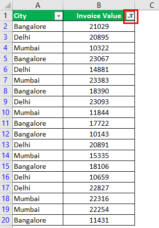
The following table shows the invoices issued to the buyers of different cities. We want to filter the data using different methods.

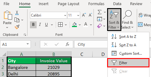
Method 1: With Filter Option Under the Home tab
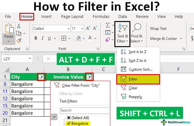
In the Home tab, there is a “filter” option under the “sort and filter” drop-down of the “editing” section, as shown in the following image.
Step 1: Select the data and click “filter” under the “sort and filter” drop-down.
Step 2: The filters are added to the selected data range. The drop-down arrows, shown within the red boxes in the following image, are filters.
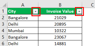
Step 3: Click the drop-down arrow of the column “city” to view the different names of the cities.
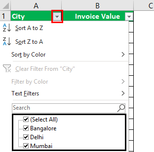
Step 4: To see the invoice values of “Delhi” only, select “Delhi” and uncheck all the remaining boxes.
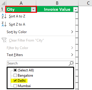
Step 5: The data for the city “Delhi” is filtered and displayed in the following image.

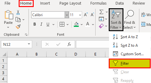
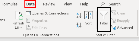
Method 2: With Filter Option Under the Data tab
In the Data tab, there is a “filter” option under the “sort and filter” section, as shown in the following image.
Method 3: With the Shortcut key
The keyboard shortcutsAn Excel shortcut is a technique of performing a manual task in a quicker way.read more are a good way to speed up the daily tasks. Select the data and add the filter using either of the following shortcuts:
- Press the keys “Shift+Ctrl+L” together.

- Press the keys “Alt+D+F+F” together.

Note: The preceding shortcuts for adding filtersUsing sorting and filtering, we can see the data category wise. With filtering data quickly you can easily navigate through menus or clicking through a mouse in less time.read more are toggle keys. Repetitive pressing helps to turn on and turn off the filters.
How to Add Filters in Excel?
We can filter numbers using advanced techniques. Let us consider some examples to understand the working of filters in Excel.
Example #1–“Number Filters” Option
Working on the data under the preceding heading (methods of filtering in Excel), we want to apply the following filters:
a. To filter column B (invoice value) for numbers greater than 10000
b. To filter column B for numbers greater than 10000 but less than 20000
Let us go through the two cases one by one.
a. Filter numbers greater than 10000
Step 1: Open the filter in column B (invoice value) by clicking on the filter symbol.
Step 2: In “number filters,” choose the “greater than” option, as shown in the following image.
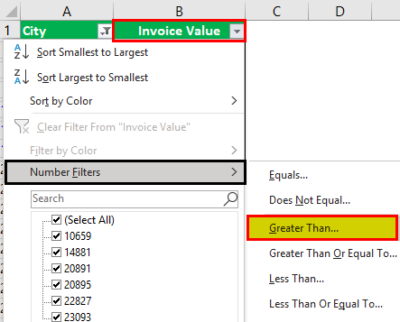
Step 3: The “custom autofilter” box appears.
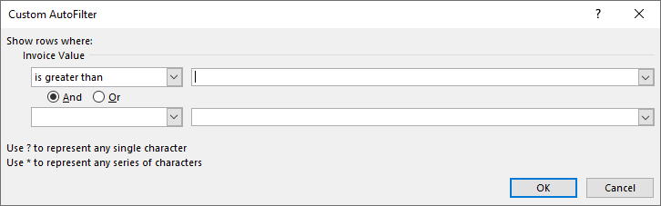
Step 4: Enter the number 10000 in the box to the right of “is greater than.”
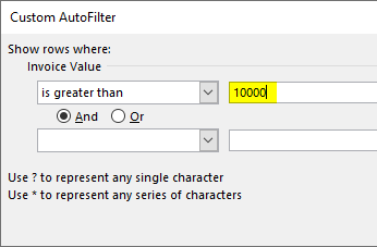
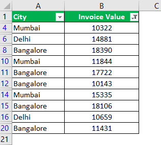
Step 5: The output displays the invoice values greater than 10000. The symbol within the red box is the filter icon. It indicates that the filter has been applied to column B.
b. Filter numbers greater than 10000 but less than 20000
Step 1: In “number filters,” choose the “greater than” option.
Step 2: In the “custom autofilter” box, select “is less than” in the second box to the left-hand side. This is shown in the following image.
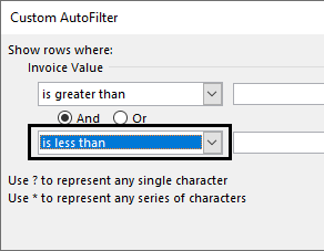
Step 3: Enter the number 10000 in the box to the right of “is greater than.” Enter the number 20000 in the box to the right of “is less than.”
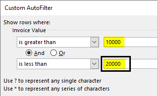
Step 4: The output displays the invoice values greater than 10000 but less than 20000.
Example #2–“Search Box” Option
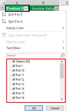
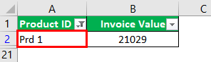
Working on the data under the preceding heading (methods of filtering in Excel), we have replaced the first column (city) with product IDs.
We want to filter the details of product ID “prd 1.”
The steps are listed as follows:
Step 1: Add filters to the columns “product ID” and “invoice value.”
Step 2: In the search boxA search box in Excel finds the needed data by typing into it, then filters the data and displays only that much info. When working with large datasheets, this simple tool may save a lot of time.read more, enter the value that is to be filtered. So, enter “prd 1.”
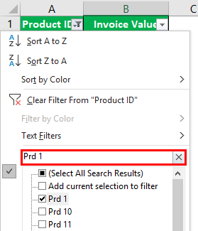
Step 3: The output displays only the filtered value from the list, as shown in the following image. Hence, we can see the invoice value of the product ID “prd 1.”
Option while you Drop Down the Filter Function
- Sort A to Z and Sort Z to A: If you wish to arrange your data ascending or descending order.
- Sort by Color: If you want to filter the data by color if a cell is filled by color.
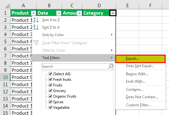
- Text filter: When you want to filter a column with some exact text or number.
- Filter cells that begin with or end with an exact character or the text
- Filter cells that contain or do not contain a given character or word anywhere in the text.
- Filter cells that are exactly equal or not equal to a detailed character.
For example:
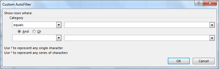
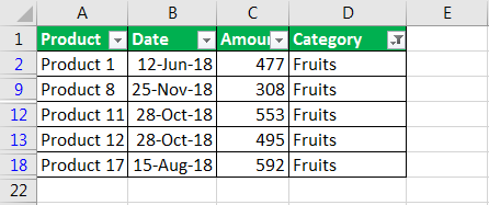
- Suppose you want to use the filter for a specific item. Click on to text filter and choose equals.
- It enables you the one dialogue, which includes a Custom Auto-Filter dialogue box.
- Enter fruits under category and click Ok.
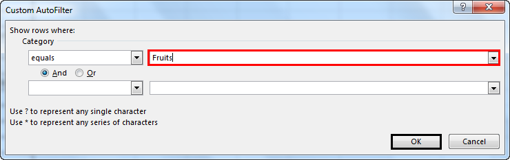
- Now you will get the data of fruits category only as shown below.
The Techniques of Filtering in Excel
The following techniques must be followed while filtering data:
- If the dataset is large, type the value to be filtered. This filters all the possible matches.
- If numerical data has to be filtered by specifying the greater than or the less than number, use the “number filters” option.
- If data has to be filtered by the color of specific rows, use the “filter by color” option.
Frequently Asked Questions
1. What are filters and how to add them in Excel?
Filtering is a technique which displays the required information and removes the unwanted data from the view. It helps the user focus on the relevant data at a given time.
The steps to add filters in Excel are listed as follows:
• Ensure that a header row appears on top of the data, specifying the column labels.
• Select the data on which filters are to be added.
• Add filters by any of the three given methods.
o Click the “filter” option under the “sort and filter” (editing section) drop-down of the Home tab.
o Click the “filter” option under the “sort and filter” section of the Data tab.
o Press the keys “Shift+Ctrl+L” or “Alt+D+F+F.”
Note: As soon as the filters are added, a drop-down arrow appears on the particular column header.
2. How to apply filters to one or more columns?
The steps to apply filters to one or more columns are listed as follows:
• Click the drop-down arrow of the column to be filtered.
• Uncheck the “select all” option which helps deselect all data.
• Select the boxes to be displayed.
• Click “Ok.”
The drop-down arrow changes to the filter icon as soon as a filter is applied. When filters are applied to multiple columns, the filter icon appears on each one of them. Hovering over the filter icon shows the filters that have been applied.
Note: The drop-down arrow on a column header indicates a filter is added. The filter icon indicates a filter has been applied.
3. How to use filters in Excel?
The filters can be applied to numbers, text values, and dates. These cases are discussed as follows:
Filter numbers
• Click on the “number filters.”
• Select any of the options like “equals,” “does not equals,” “greater than,” “less than,” “between,” “above average,” and so on.
• Specify the required fields in the dialog box that appears. This box may or may not be displayed.
For instance, in “equals,” enter the number against which the values should be compared. The filtered results show the matching numerical values.
Filter text and date values
• To filter text and date values, select “text filters” and “date filters” from the respective drop-down arrows.
• The “text filters” allow filtering text strings which contain specific characters or words. The “date filters” allow filtering dates for a particular year, month, week, and so on.
Note: The “plus” and the “minus” sign of the date filters are used for expanding and collapsing the various levels respectively.
Recommended Articles
This has been a guide to Filter in Excel. Here we discuss how to use/add filters in excel along with step by step examples and a downloadable template. You may learn more about Excel from the following articles –
- VBA FilterThe VBA Filter tool is used to sort out or fetch the desired data. However, this function accepts optional arguments, and the only required argument is an expression that covers the range, such as worksheets(«Sheet1»). Range(“A1”).read more
- How to Filter Pivot Table?By right-clicking on the pivot table, we can access the pivot table filter option. Another approach is to use the filter options available in the pivot table fields.read more
- Advanced Filter in ExcelThe advanced filter is different from the auto filter in Excel. This feature is not like a button that one can use with a single click of the mouse. To use an advanced filter, we have to define criteria for the auto filter and then click on the “Data” tab. Then, in the advanced section for the advanced filter, we will fill our criteria for the data.read more
- Types of Filters in Power BIThe filter function in Power BI is more commonly used to read data or reports based on multiple criteria. Visual level filters, page-level filters, report-level filters, drill-through filters, and so on are all available filters in Power Bi.read more
Disclosure: Some of the links on this site are affiliate links, meaning that if you click on one of the links and purchase an item, I may receive a commission. All opinions however are my own.
Excel program is one of the most used spreadsheet programs.
If you don’t know its advantages, then let me tell you, with the excel program you can do various calculations, advanced filter excels, maintain data, perform mathematical operations, auto filter excel, create spreadsheets, and lots more features are there provided by excel program.
Today, we will be discussing the procedure of How to filter in excel. If you don’t know what actually a filter function is, the basic intro is given below. Have a look at that.
Filtering in excel simply means displaying certain data. In other words, filtering means setting a condition, so that only certain data is displayed.
For example, when you have a large number of data, and you want to display particular information, then all you will have to do is, filter the data. Once the data is filtered, and the condition is set to show the certain data, the only data that you chose to filter would display.
How to Filter in Excel
In excel filter multiple columns can also be done. In the article, we will let you know the complete step-by-step guide to filter the data. Along with the filtering in excel. We will be also telling you the procedure for advance filtering.
Check out the guide and let me know, how do you find it. The steps are described below. If you face any difficulty in any step, do ask that by dropping the comment below.
Step 1: First of all, enter the data in the excel sheet you want to filter. For example, as you can see below, in the image I have mentioned some data. In the data below, I have mentioned the rows with Sr. No., Customer ID, amount, Country, and years. Check the image below.
Now here, we have to filter the data. For example, I want to display the Country UK, along with the year 2015. So how do we do that? I have shown it below. Simply follow the second step.
Step 2: In order to apply the filter function to the sheet, first select the rows you want to apply the filter function to, and then go to the Data tab from the menu bar, and select Filter. The screenshot is given below.
Step 3: As sooner you click on the filter option, a drop-down arrow will appear in the header cell for each column. Check out the image below.
Remember, In order for filtering data properly, your worksheet should include a header row, it is used to identify the name of each column. As in our example sheet, we have taken the header column as Sr. No., Customer ID, amount, Country, and years.
Step 4: Now, as we have to filter the Country UK, we will have to click n the drop-down arrow from the country column. Once done, apply the same procedure for the year or for any data you want to filter.
As sooner you will click on the arrow button. you will see a screen as I have mentioned below.
Step 5: As you can see in the above image, there are basically three options appearing. UK, USA, and Select All. If there would be more countries, all would have been showing in the list. But as I have mentioned only two of the countries, we have to select from them.
As I told you above, I want to display the list of Uk, I will check the box of UK and Uncheck the rest of the checkboxes. As sooner I will do that, the only country UK will start displaying.
And the filtering arrow in the table header changes to this icon. This indicates a filter is applied. To make any changes or clear the filter, click on this icon.
I have mentioned the screenshot below. If you finding difficulty in understanding, keep referring to the screenshots.
Step 6: And you are done. This is how we filter data in an excel program.
This was the first method to perform a filter in excel. Another method is given below.
Step 1: To perform the filter, select the cell first. Once done, right-click on it and then click Filter. See the screenshot below.

Step 2: As it is clearly visible in the above image, after clicking on the filter option, a small drop-down will appear. All you have to do is click on the Filter by Selected Cell’s Value. And you are done!!
So, these were the basic two methods to perform filters in excel. I hope you got all the steps clear. You must have. Along with the steps, I also have provided the screenshot. But still, if you find any difficulty you can drop the comment below.
Ok, so this was about how to filter in excel. The methods I shown above are simple filtering methods. But below, I am going to show you how excel advanced filter is performed.
However, an advanced filter in excel is not as easy as simple filtering. You may find advanced filtering a little complex than the simple filter. But, once you manage to perform the advanced filter, you may find it more beneficial. Check out the given below.
Step 1: To perform advanced filter in excel. first, click on the Data tab from the menu bar. And then select Advanced.
Step 2: After you click on the advanced option, the Advanced Filter dialog box will open up. And you will see a screen as I have mentioned below.

Now here, all you have to do is fill in the details, and then click the OK button to filter the data. And the data would be filtered.
So, this how-to filter in excel. I hope the given guide will help you to perform a filter in your excel sheet. In case, of any confusion, you can drop your comment. We will try to reach out to you as soon as possible.
If you know any other method to perform filter in excel, you can share it with us.
Also, do check out our previous guide excel by clicking here. You can also consider sharing the guide if you find it useful.
Quick Links
- How To Multiply In Excel
- How To Create A Drop Down List in Excel
- How To Update Google Chrome A Basic Guide To Update Google Chrome
Содержание
- Quick start: Filter data by using an AutoFilter
- Next steps
- FILTER function
- Examples
- Need more help?
- Filter data in a range or table
- Try it!
- Filter a range of data
- Filter data in a table
- Filter data in a range or table
- Filter a range of data
- Filter data in a table
- Related Topics
- Filter data in a table
- Filter a range of data
- Filtering options for tables or ranges
- To clear a filter from a column
- To remove all the filters from a table or range
- Need more help?
Quick start: Filter data by using an AutoFilter
By filtering information in a worksheet, you can find values quickly. You can filter on one or more columns of data. With filtering, you can control not only what you want to see, but what you want to exclude. You can filter based on choices you make from a list, or you can create specific filters to focus on exactly the data that you want to see.
You can search for text and numbers when you filter by using the Search box in the filter interface.
When you filter data, entire rows are hidden if values in one or more columns don’t meet the filtering criteria. You can filter on numeric or text values, or filter by color for cells that have color formatting applied to their background or text.

Select the data that you want to filter
On the Data tab, in the Sort & Filter group, click Filter.
Click the arrow  in the column header to display a list in which you can make filter choices.
Note Depending on the type of data in the column, Microsoft Excel displays either Number Filters or Text Filters in the list.

Filter by selecting values or searching
Selecting values from a list and searching are the quickest ways to filter. When you click the arrow in a column that has filtering enabled, all values in that column appear in a list.

1. Use the Search box to enter text or numbers on which to search
2. Select and clear the check boxes to show values that are found in the column of data
3. Use advanced criteria to find values that meet specific conditions
To select by values, in the list, clear the (Select All) check box. This removes the check marks from all the check boxes. Then, select only the values you want to see, and click OK to see the results.
To search on text in the column, enter text or numbers in the Search box. Optionally, you can use wildcard characters, such as the asterisk ( *) or the question mark ( ?). Press ENTER to see the results.

Filter data by specifying conditions
By specifying conditions, you can create custom filters that narrow down the data in the exact way that you want. You do this by building a filter. If you’ve ever queried data in a database, this will look familiar to you.
Point to either Number Filters or Text Filters in the list. A menu appears that allows you to filter on various conditions.
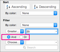
Choose a condition and then select or enter criteria. Click the And button to combine criteria (that is, two or more criteria that must both be met), and the Or button to require only one of multiple conditions to be met.
Click OK to apply the filter and get the results you expect.
Next steps
Experiment with filters on text and numeric data by trying the many built-in test conditions, such as Equals, Does Not Equal, Contains, Greater Than, and Less Than. For more information, see Filter data in a range or table.
Note Some of these conditions apply only to text, and others apply only to numbers.
Create a custom filter that uses multiple criteria. For more information, see Filter by using advanced criteria.
Источник
FILTER function
The FILTER function allows you to filter a range of data based on criteria you define.
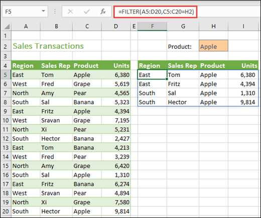
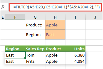
In the following example we used the formula =FILTER(A5:D20,C5:C20=H2,»») to return all records for Apple, as selected in cell H2, and if there are no apples, return an empty string («»).
The FILTER function filters an array based on a Boolean (True/False) array.
The array, or range to filter
A Boolean array whose height or width is the same as the array
The value to return if all values in the included array are empty (filter returns nothing)
An array can be thought of as a row of values, a column of values, or a combination of rows and columns of values. In the example above, the source array for our FILTER formula is range A5:D20.
The FILTER function will return an array, which will spill if it’s the final result of a formula. This means that Excel will dynamically create the appropriate sized array range when you press ENTER. If your supporting data is in an Excel table, then the array will automatically resize as you add or remove data from your array range if you’re using structured references. For more details, see this article on spilled array behavior.
If your dataset has the potential of returning an empty value, then use the 3rd argument ( [if_empty]). Otherwise, a #CALC! error will result, as Excel does not currently support empty arrays.
If any value of the include argument is an error (#N/A, #VALUE, etc.) or cannot be converted to a Boolean, the FILTER function will return an error.
Excel has limited support for dynamic arrays between workbooks, and this scenario is only supported when both workbooks are open. If you close the source workbook, any linked dynamic array formulas will return a #REF! error when they are refreshed.
Examples
FILTER used to return multiple criteria
In this case, we’re using the multiplication operator (*) to return all values in our array range (A5:D20) that have Apples AND are in the East region: =FILTER(A5:D20,(C5:C20=H1)*(A5:A20=H2),»»).
FILTER used to return multiple criteria and sort
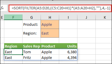
In this case, we’re using the previous FILTER function with the SORT function to return all values in our array range (A5:D20) that have Apples AND are in the East region, and then sort Units in descending order: =SORT(FILTER(A5:D20,(C5:C20=H1)*(A5:A20=H2),»»),4,-1)
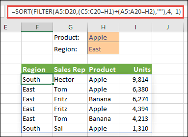
In this case, we’re using the FILTER function with the addition operator (+) to return all values in our array range (A5:D20) that have Apples OR are in the East region, and then sort Units in descending order: =SORT(FILTER(A5:D20,(C5:C20=H1)+(A5:A20=H2),»»),4,-1).
Notice that none of the functions require absolute references, since they only exist in one cell, and spill their results to neighboring cells.
Need more help?
You can always ask an expert in the Excel Tech Community or get support in the Answers community.
Источник
Filter data in a range or table
Try it!
Use filters to temporarily hide some of the data in a table, so you can focus on the data you want to see.
Filter a range of data
Select any cell within the range.
Select Data > Filter.

Select the column header arrow  .
.
Select Text Filters or Number Filters, and then select a comparison, like Between.

Enter the filter criteria and select OK.

Filter data in a table
When you Create and format tables, filter controls are automatically added to the table headers.
Select the column header arrow for the column you want to filter.
Uncheck (Select All) and select the boxes you want to show.

The column header arrow changes to a  Filter icon. Select this icon to change or clear the filter.
Источник
Filter data in a range or table
Use AutoFilter or built-in comparison operators like «greater than» and “top 10” in Excel to show the data you want and hide the rest. Once you filter data in a range of cells or table, you can either reapply a filter to get up-to-date results, or clear a filter to redisplay all of the data.
Use filters to temporarily hide some of the data in a table, so you can focus on the data you want to see.
Filter a range of data
Select any cell within the range.
Select Data > Filter.
Select the column header arrow .
Select Text Filters or Number Filters, and then select a comparison, like Between.
Enter the filter criteria and select OK.
Filter data in a table
When you put your data in a table, filter controls are automatically added to the table headers.
Select the column header arrow for the column you want to filter.
Uncheck (Select All) and select the boxes you want to show.
The column header arrow changes to a Filter icon. Select this icon to change or clear the filter.
Filtered data displays only the rows that meet criteria that you specify and hides rows that you do not want displayed. After you filter data, you can copy, find, edit, format, chart, and print the subset of filtered data without rearranging or moving it.
You can also filter by more than one column. Filters are additive, which means that each additional filter is based on the current filter and further reduces the subset of data.
Note: When you use the Find dialog box to search filtered data, only the data that is displayed is searched; data that is not displayed is not searched. To search all the data, clear all filters.
The two types of filters
Using AutoFilter, you can create two types of filters: by a list value or by criteria. Each of these filter types is mutually exclusive for each range of cells or column table. For example, you can filter by a list of numbers, or a criteria, but not by both; you can filter by icon or by a custom filter, but not by both.
Reapplying a filter
To determine if a filter is applied, note the icon in the column heading:
A drop-down arrow means that filtering is enabled but not applied.
When you hover over the heading of a column with filtering enabled but not applied, a screen tip displays «(Showing All)».
A Filter button means that a filter is applied.
When you hover over the heading of a filtered column, a screen tip displays the filter applied to that column, such as «Equals a red cell color» or «Larger than 150».
When you reapply a filter, different results appear for the following reasons:
Data has been added, modified, or deleted to the range of cells or table column.
Values returned by a formula have changed and the worksheet has been recalculated.
Do not mix data types
For best results, do not mix data types, such as text and number, or number and date in the same column, because only one type of filter command is available for each column. If there is a mix of data types, the command that is displayed is the data type that occurs the most. For example, if the column contains three values stored as number and four as text, the Text Filters command is displayed .
Filter data in a table
When you put your data in a table, filtering controls are added to the table headers automatically.
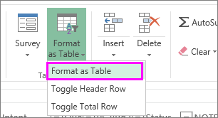
Select the data you want to filter. On the Home tab, click Format as Table, and then pick Format as Table.
In the Create Table dialog box, you can choose whether your table has headers.
Select My table has headers to turn the top row of your data into table headers. The data in this row won’t be filtered.
Don’t select the check box if you want Excel for the web to add placeholder headers (that you can rename) above your table data.
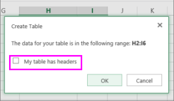
To apply a filter, click the arrow in the column header, and pick a filter option.
Filter a range of data
If you don’t want to format your data as a table, you can also apply filters to a range of data.
Select the data you want to filter. For best results, the columns should have headings.
On the Data tab, choose Filter.
Filtering options for tables or ranges
You can either apply a general Filter option or a custom filter specific to the data type. For example, when filtering numbers, you’ll see Number Filters, for dates you’ll see Date Filters, and for text you’ll see Text Filters. The general filter option lets you select the data you want to see from a list of existing data like this:
Number Filters lets you apply a custom filter:
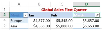
In this example, if you want to see the regions that had sales below $6,000 in March, you can apply a custom filter:
Click the filter arrow next to March > Number Filters > Less Than and enter 6000.
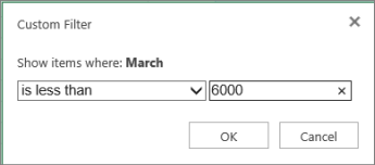
Excel for the web applies the filter and shows only the regions with sales below $6000.
You can apply custom Date Filters and Text Filters in a similar manner.
To clear a filter from a column
Click the Filter button next to the column heading, and then click Clear Filter from .
To remove all the filters from a table or range
Select any cell inside your table or range and, on the Data tab, click the Filter button.
This will remove the filters from all the columns in your table or range and show all your data.
Click a cell in the range or table that you want to filter.
On the Data tab, click Filter.

Click the arrow  in the column that contains the content that you want to filter.
Under Filter, click Choose One, and then enter your filter criteria.
You can apply filters to only one range of cells on a sheet at a time.
When you apply a filter to a column, the only filters available for other columns are the values visible in the currently filtered range.
Only the first 10,000 unique entries in a list appear in the filter window.
Click a cell in the range or table that you want to filter.
On the Data tab, click Filter.
Click the arrow in the column that contains the content that you want to filter.
Under Filter, click Choose One, and then enter your filter criteria.
In the box next to the pop-up menu, enter the number that you want to use.
Depending on your choice, you may be offered additional criteria to select:
You can apply filters to only one range of cells on a sheet at a time.
When you apply a filter to a column, the only filters available for other columns are the values visible in the currently filtered range.
Only the first 10,000 unique entries in a list appear in the filter window.
Instead of filtering, you can use conditional formatting to make the top or bottom numbers stand out clearly in your data.
You can quickly filter data based on visual criteria, such as font color, cell color, or icon sets. And you can filter whether you have formatted cells, applied cell styles, or used conditional formatting.
In a range of cells or a table column, click a cell that contains the cell color, font color, or icon that you want to filter by.
On the Data tab, click Filter .
Click the arrow  in the column that contains the content that you want to filter.
Under Filter, in the By color pop-up menu, select Cell Color, Font Color, or Cell Icon, and then click a color.
This option is available only if the column that you want to filter contains a blank cell.
Click a cell in the range or table that you want to filter.
On the Data toolbar, click Filter.
Click the arrow in the column that contains the content that you want to filter.
In the (Select All) area, scroll down and select the (Blanks) check box.
You can apply filters to only one range of cells on a sheet at a time.
When you apply a filter to a column, the only filters available for other columns are the values visible in the currently filtered range.
Only the first 10,000 unique entries in a list appear in the filter window.
Click a cell in the range or table that you want to filter.
On the Data tab, click Filter .
Click the arrow in the column that contains the content that you want to filter.
Under Filter, click Choose One, and then in the pop-up menu, do one of the following:
To filter the range for
Rows that contain specific text
Contains or Equals.
Rows that do not contain specific text
Does Not Contain or Does Not Equal.
In the box next to the pop-up menu, enter the text that you want to use.
Depending on your choice, you may be offered additional criteria to select:
Filter the table column or selection so that both criteria must be true
Filter the table column or selection so that either or both criteria can be true
Click a cell in the range or table that you want to filter.
On the Data toolbar, click Filter .
Click the arrow in the column that contains the content that you want to filter.
Under Filter, click Choose One, and then in the pop-up menu, do one of the following:
The beginning of a line of text
The end of a line of text
Cells that contain text but do not begin with letters
Does Not Begin With.
Cells that contain text but do not end with letters
Does Not End With.
In the box next to the pop-up menu, enter the text that you want to use.
Depending on your choice, you may be offered additional criteria to select:
Filter the table column or selection so that both criteria must be true
Filter the table column or selection so that either or both criteria can be true
Wildcard characters can be used to help you build criteria.
Click a cell in the range or table that you want to filter.
On the Data toolbar, click Filter.
Click the arrow in the column that contains the content that you want to filter.
Under Filter, click Choose One, and select any option.
In the text box, type your criteria and include a wildcard character.
For example, if you wanted your filter to catch both the word «seat» and «seam», type sea?.
Do one of the following:
Any single character
For example, sm?th finds «smith» and «smyth»
Any number of characters
For example, *east finds «Northeast» and «Southeast»
A question mark or an asterisk
For example, there
Do any of the following:
Remove specific filter criteria for a filter
Click the arrow in a column that includes a filter, and then click Clear Filter.
Remove all filters that are applied to a range or table
Select the columns of the range or table that have filters applied, and then on the Data tab, click Filter.
Remove filter arrows from or reapply filter arrows to a range or table
Select the columns of the range or table that have filters applied, and then on the Data tab, click Filter.
When you filter data, only the data that meets your criteria appears. The data that doesn’t meet that criteria is hidden. After you filter data, you can copy, find, edit, format, chart, and print the subset of filtered data.
Table with Top 4 Items filter applied
Filters are additive. This means that each additional filter is based on the current filter and further reduces the subset of data. You can make complex filters by filtering on more than one value, more than one format, or more than one criteria. For example, you can filter on all numbers greater than 5 that are also below average. But some filters (top and bottom ten, above and below average) are based on the original range of cells. For example, when you filter the top ten values, you’ll see the top ten values of the whole list, not the top ten values of the subset of the last filter.
In Excel, you can create three kinds of filters: by values, by a format, or by criteria. But each of these filter types is mutually exclusive. For example, you can filter by cell color or by a list of numbers, but not by both. You can filter by icon or by a custom filter, but not by both.
Filters hide extraneous data. In this manner, you can concentrate on just what you want to see. In contrast, when you sort data, the data is rearranged into some order. For more information about sorting, see Sort a list of data.
When you filter, consider the following guidelines:
Only the first 10,000 unique entries in a list appear in the filter window.
You can filter by more than one column. When you apply a filter to a column, the only filters available for other columns are the values visible in the currently filtered range.
You can apply filters to only one range of cells on a sheet at a time.
Note: When you use Find to search filtered data, only the data that is displayed is searched; data that is not displayed is not searched. To search all the data, clear all filters.
Need more help?
You can always ask an expert in the Excel Tech Community or get support in the Answers community.
Источник
This post will guide you how to extracts matched values using FILTER function in Microsoft Excel 365. And also will introduce that how to use FILTER function with same examples in Excel 365.
Table of Contents
- Excel Filter Function
- Entering FILTER Formula in Excel
- Excel filtering by a single criteria
- Example 1: How to use a number as a filter
- Example 2: How to filter in Excel by a cell value
- Example 3: Using Excel’s text filter
- Example 4: Using NOT EQUAL TO as a FILTER condition in Excel
- Example 5: How to use the date filter in Excel
- Example 6: Filtering by date in Excel
- Example 7: Filtering based on two Conditions
- Example 8: Filtering Based on Two Conditions using OR Logic
- Example 9: Filter Data in Excel from Another Sheet
- Example 10: Providing Maximum Number of Rows of Filtered Data
- Conclusion
- Related Functions
The FILTER function “filters” a set of data according to the conditions specified. The outcome is an array of values that match those in the original range. Simply said, the FILTER function extracts matched records from a collection of data using one or more logical checks. The include argument specifies logical tests, which might encompass a wide variety of formula conditions. For instance, FILTER may match data from a given year or month, data containing specific content, or numbers above a specified threshold.
=FILTER(array,include,[if empty])
Three parameters are required for the FILTER function: array, include, and if empty.
Where:
- Array – This is required argument. The range or array to filter is specified by array.
- Include – This is required argument. Include one or more logical tests in the include These tests should return TRUE or FALSE depending on the array values evaluated.
- If_empty – This is option argument. The last input, if empty, specifies the value to return if FILTER does not discover any matching values. Typically, this is a message along the lines of “No records found,” although other values may also be returned. To show nothing, provide an empty string (“”).
Entering FILTER Formula in Excel
FILTER provides dynamic results. When the values in the source data change or the size of the source data array changes, the FILTER results are updated automatically. The results of FILTER will “leak” into numerous cells on the worksheet.
To filter data in Excel using the FILTER function, follow these steps:
Step1: To begin your filter formula, enter =FILTER(.
Step2: Enter the address for the range of cells containing the data you want to filter, for example, A2:C10.
Step3: Type a comma, followed by the filter's condition, such as B2:B20>3 (To specify a condition, type the address of the “criteria column,” such as C1:C, followed by an operator symbol such as greater than (>), and finally the criterion, such as the number 3.
Step4: Complete the parenthesis with a closing parenthesis and then hit enter on the keyboard. Your full formula will appear as follows: =FILTER(A2:C10, B2:B20>3)
I’ll begin with the fundamentals of utilizing the FILTER function, and then demonstrate some more advanced uses of the FILTER function. This article discusses the FILTER function as a formula entered into spreadsheet cells, not the filter command accessible from the toolbar and pop-up menus.
While using the FILTER function in Excel is almost identical to using it in Google Sheets, there are some subtle variations.
Excel filtering by a single criteria
To begin, let’s review how to use Excel’s FILTER function in its simplest version, with a single condition/criteria.
I’ll demonstrate how to filter data using a number, a cell value, a text string, or a date… and I’ll also demonstrate how to utilize a variety of “operators” in the filter condition (Less than, Equal to, etc…).
Example 1: How to use a number as a filter
In this first demonstration of how to use the filter tool in Excel, we have a list of students and their grades and wish to create a filtered list of only students with flawless grades.
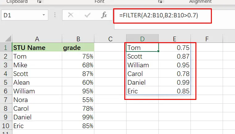
The assignment: Display a list of students and their grades, but only those who have earned an A.
The reasoning: Filter the range A2:B10 for values larger than 0.7 in the column B2:B10 (70 percent ). Then you can use the following FILTER formula,type:
=FILTER(A2:B10, B2:B10 >0.7)
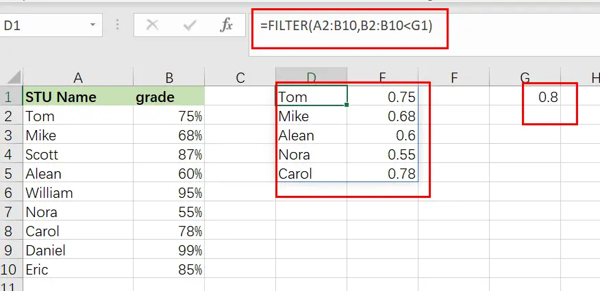
Example 2: How to filter in Excel by a cell value
In this excel filter function example, we want to do the same thing as stated before, but rather than inputting the condition straight into the formula, we’re going to use a cell reference.
When you filter in Excel by a cell value, your sheet is configured in such a way that you may alter the value in the cell at any moment, which updates the value to which the filter criterion is tied.
In this example, rather than explicitly entering the value “0.8” into the formula, the filter criterion is set to cell G1, which contains the “0.8” value.
The assignment: Display a list of students and their grades, but only those with a score of less than 80%.
The reasoning: Filter the range A2:B10 to the extent that B2:B10 is smaller than the value supplied in column G1 (0.8).
You can use the following FILTER formula, type:
=FILTER(A2:B10, B2:B10 <G1)
Example 3: Using Excel’s text filter
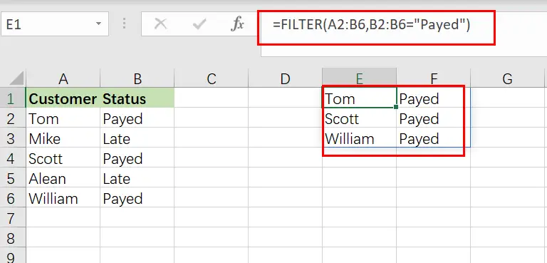
In this example, we’ll utilize a text string as the filter formula’s criterion. This is fairly similar to using a number, except that the text to filter must be enclosed in quote marks.
We are filtering a list of customers and their payment status in this instance, and we want to present just customers with a payment status of “Payed“.
The objective is to provide a list of clients that have paid on their payments.
The reasoning: Filter the range A2:B6 by substituting the string “ Payed ” for B2:B6.
The following formula: In this example, the formula below is typed in the cell (E1).
=FILTER(A3:B12, B2:B6=" Payed ")
Example 4: Using NOT EQUAL TO as a FILTER condition in Excel
Now that you have a working knowledge of how to use the filter function in Excel, here is another example of filtering by a string of text, but this time we will use the “not equal” operator (<>) to demonstrate how to filter a range and return data that is NOT equal to the criteria you set.
Additionally, we will utilize a bigger data set in this example to show a more comprehensive usage of the FILTER function in the real world.
You may be surprised at how often a circumstance arises in which you need to filter data that is “not equal to” a certain number or piece of text.
In this example, we’ll use a report/spreadsheet to display data from sales calls that occur at your organization, and we’ll filter the data to exclude a certain sales person (Scott) from the result.
The assignment: Display sales call statistics for all sales representatives except ” Scott “.
The reasoning: Filter the range A2:C10 for values A2:A10 that DO NOT match the string “Scott “.
The following formula: In this example, the formula below is typed in the cell (E1).
=FILTER(A2:C10, A2:A10 <>"Scott")
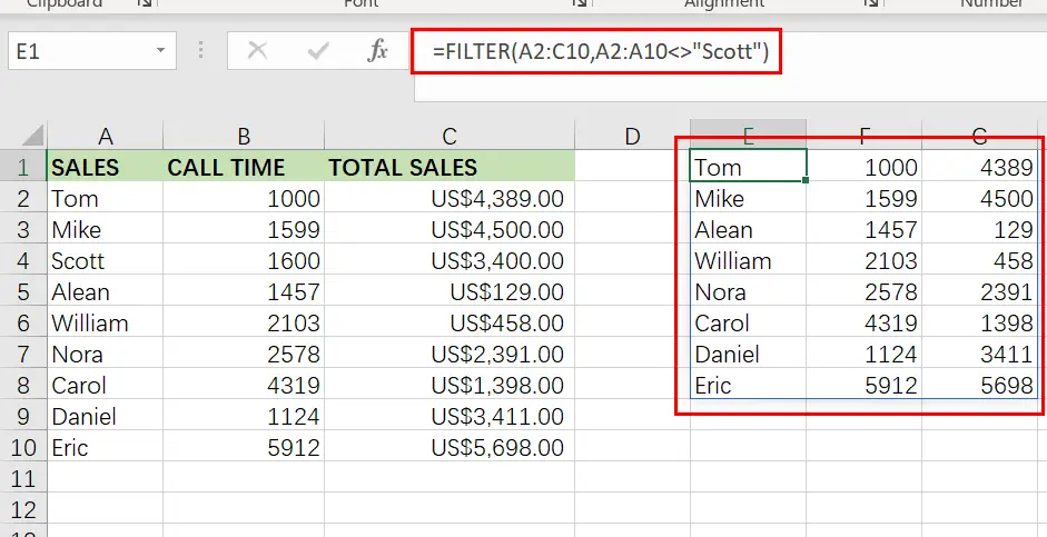
Take note that the filtered data on the right side of the figure above does not include any of Scott ‘s rows/calls.
Example 5: How to use the date filter in Excel
Filtering in Excel by a date may be accomplished in a few different methods, which I will demonstrate below. If you attempt to put a date into the FILTER function in the same way that you would typically type into a cell, the formula will fail to operate properly.
Therefore, you may either enter the date you want to filter into a cell and then reference that cell in your formula… Alternatively, you may use the DATE function.
When filtering by date, the same operators (>, =, etc…) are available as they are in other FILTER function applications. Each individual day/date in Excel is merely a number that has been formatted differently. In Excel, for example, the date “01/30/2022” is just the serial number “44591” formatted as a date. Each time you add a day to the calendar, this number increases by one… For example, “44591” “44592” “44593”
Thus, if one date is farther in the future, it might be regarded “greater than” another. In contrast, if one date is farther in the past, it might be considered to be “less than” another.
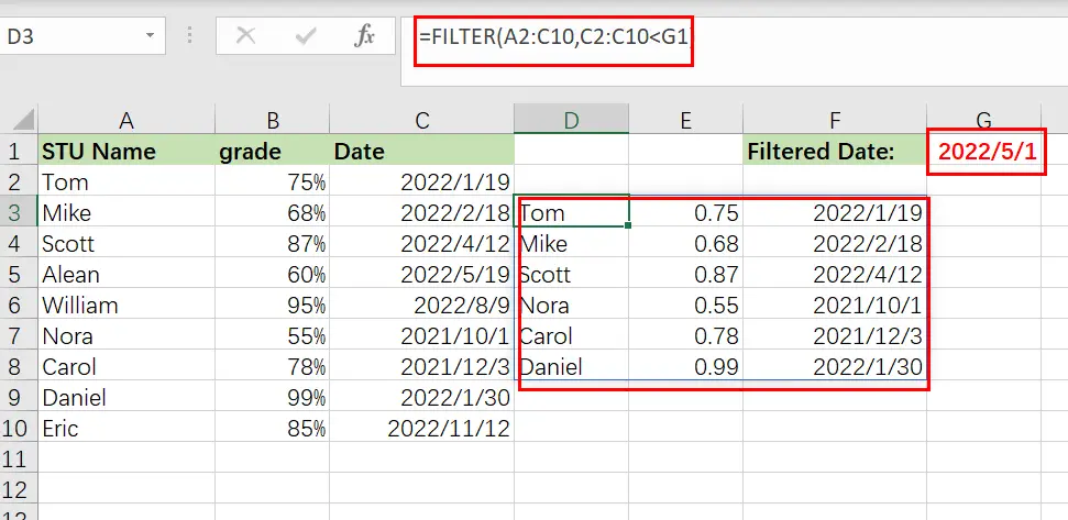
In this example, we’ll use a cell reference to filter on a date. This is identical to the example discussed in Example 2, except that we are dealing with dates instead of percentages.
Consider the following scenario: we want to filter a list of students, their exam results, and the dates on which the tests were administered… and we wish to display only tests conducted before to June (05/01/2022).
=FILTER(A2:C10, C2:C10 <G1)
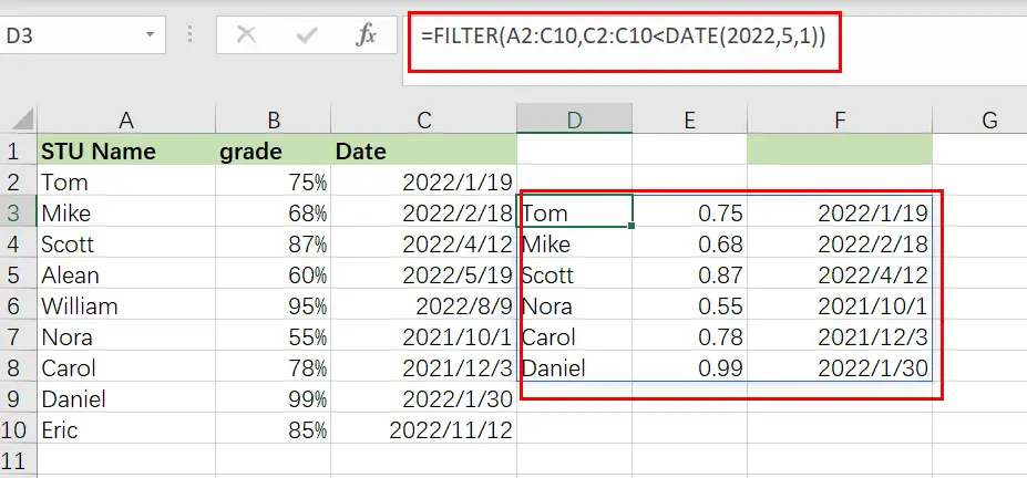
Example 6: Filtering by date in Excel
In this example of date filtering in Excel, we’ll use the same data as in the previous one and attempt to obtain the same results… however, instead of referencing a cell, we’ll utilize the DATE function, which allows you to put the date straight into the FILTER function.
When using the DATE function to provide a date, you must first input the year, followed by the month and finally the day… each denoted with a comma (shown below).
The assignment: Display only exams given before to May
The reasoning: Filter the range A2:C10 so that C2:C10 is less than or equal to the date (05/01/2022).
The following formula: In this example, the formula below is typed in the cell (D3).
=FILTER(A2:C10,C2:C10<DATE(2022,5,1))
Example 7: Filtering based on two Conditions
When utilizing the Excel FILTER function, you may want to produce data that fits many criteria. I’ll demonstrate two methods for filtering by several criteria in Excel, depending on the scenario and the desired behavior of the calculation.
The conventional method of adding another condition to your filter function (as shown by the Excel formula syntax) allows you to provide a second condition, where both the first AND second conditions must be fulfilled in order for the filter output to be returned.
However, I will demonstrate how to make a little tweak to the function so that you may choose to return/display in the filter function’s output/destination a second condition where EITHER condition might be satisfied. (To utilize AND logic, separate the conditions with an asterisk, or use a plus symbol to separate the criteria.)
In this example, we’re going to filter a collection of data and show those rows that satisfy BOTH the first and second conditions.
To utilize a second condition in this manner (using AND logic), just insert it after the first condition in the formula, separated by an asterisk (*). Each condition must be included in a separate pair of parentheses.
When a filter formula is used with several conditions, the columns referenced in each condition must be distinct.
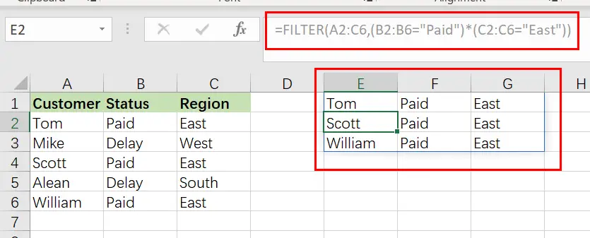
In this case, we’d want to filter a list of clients based on their payment status and region… and to display those customers who are both current members AND paid on their payment status.
The objective is to provide a list of customers who are paid on payments, but only those who are in East region.
The reasoning: Filter the range A2:C6 such that B2:B6 equals the text “Paid,” AND C2:C6 equals the text “East“.
The following formula: In this example, the formula below is typed in the blue cell (E1).
=FILTER(A2:C6,( B2:B6="Paid")*( C2:C6 ="East"))
Example 8: Filtering Based on Two Conditions using OR Logic
In this example, we’re going to filter a collection of data and show those rows that satisfy either the first OR the second criterion.
To utilize a second condition in this manner (using OR logic), just insert it after the first condition in the formula, separated by a plus sign. Each condition must be included in a separate pair of parentheses (shown below).
When used in this manner, the FILTER formula allows you to choose criteria from the same or separate columns.
In this case, we’re filtering the same customer data as in the previous example, but this time we’re displaying a list of customers who either are in East region OR have paid on a payment. This will generate a list of clients to whom a payment notification have paid… whether they are current members or east region who have paid on their last payment.
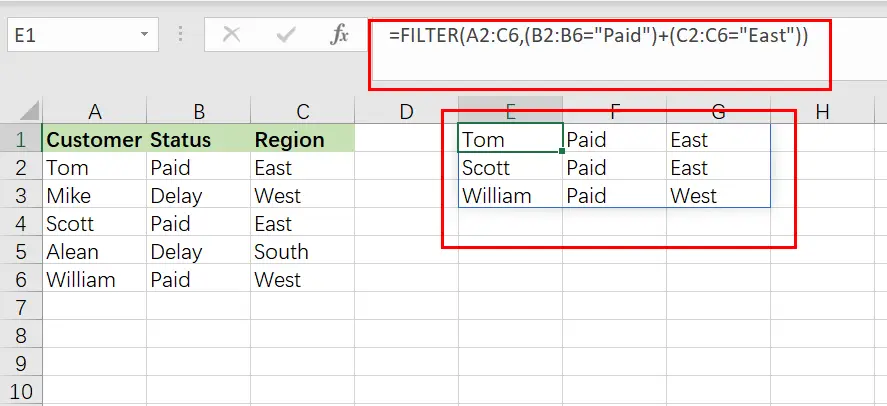
The objective is to provide a list of customers who are in East region, as well as customers who have paid on payments regardless of whether they are in East region.
The following formula: In this example, the formula below is typed in the cell (E1).
=FILTER(A2:C6, (B2:B6="Paid ")+(C2:C6=" East ")
Example 9: Filter Data in Excel from Another Sheet
You may often encounter instances in Excel when you need to filter data from another sheet, where your raw unfiltered data is on one tab and your filter formula is on another sheet.
This may be accomplished by simply referring to a certain sheet’s name when providing the filter’s ranges. Thus, while you would typically give a range such as “A1:B4,” when referring another sheet when filtering, you indicate the sheet name by preceding the range with the sheet name and an exclamation mark, as in “SheetName!A1:B4“.
However, if the sheet name contains a space, an apostrophe must be used before and after the sheet name, as in "Sheet Name!" A1:B4.
The following is an example of how to filter data in Excel from a separate sheet, where the filter formula is located on a different sheet than the source range.
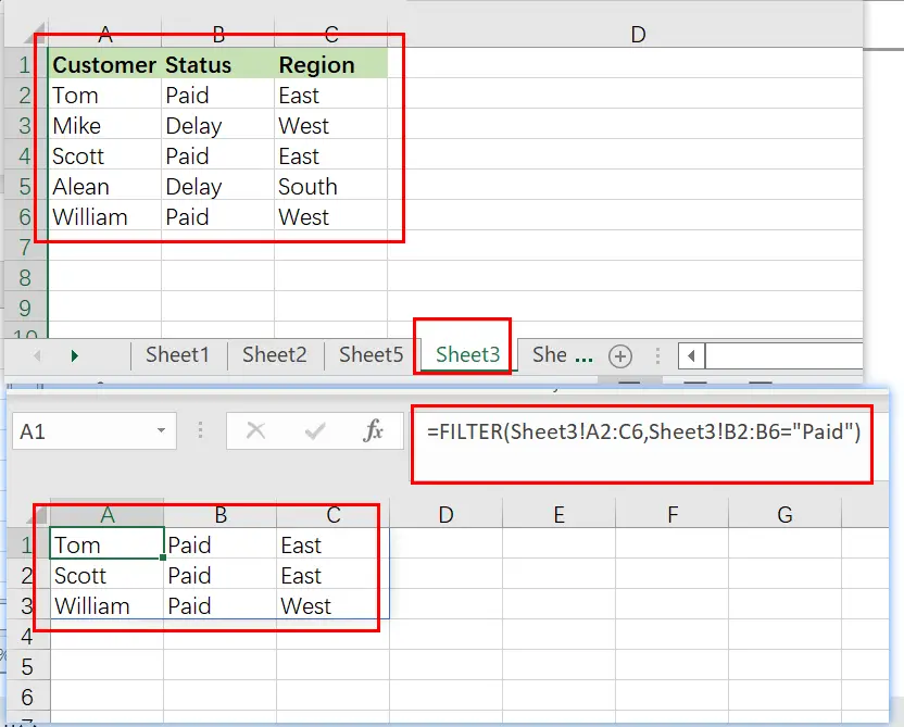
Consider the following scenario: On one sheet, you have a list of customers and their payment status, and you wish to present a filtered list of paid customer on another sheet.
The job is to filter the list of customers on the Sheet3 and to display a separate list of customer names with a pay status on another worksheet.
The reasoning: Filter the range using the Sheet3‘ command! A2:C6, where ‘ Sheet3′ is the range! B2:B6 corresponds to the phrase “Paid“.
The following formula: In this example, the formula below is typed in the cell (A3).
=FILTER(Sheet3! A2:C6, Sheet3!B2:B6="Paid")
Example 10: Providing Maximum Number of Rows of Filtered Data
If your FILTER formula provides a large number of rows but your worksheet is restricted in space and you are unable to erase the data below, you may limit the amount of rows returned by the FILTER function.
Let us demonstrate how it works using a simple formula that filter data that grade is less than 0.7 from filter value in Cell F1:
=FILTER(A2:C10, B2:B10<F1)
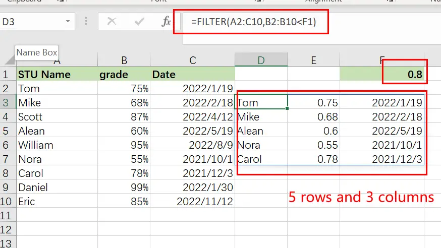
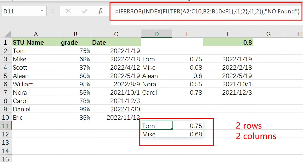
The preceding formula produces all records that it discovers, in this instance five rows. However, imagine you only have room for two. To output just the first two rows discovered, follow these steps:
Step1: Incorporate the FILTER formula into the INDEX function’s array parameter
Step2: Use a vertical array constant such as 1;2 as the row num input to INDEX. It specifies the number of rows to return (2 in our case).
Step3: Use a horizontal array constant such as 1,2 for the column num parameter. It defines the columns that should be returned (the first 2 columns in this example).
Step4: To account for any mistakes caused by the absence of data meeting your criteria, you may wrap your calculation in the IFERROR function.
The entire excel filter formula is as follows:
=IFERROR(INDEX(FILTER(A2:C10, B2:B10<F1), {1;2},{1,2}), "No Found")
Conclusion
This section discusses the FILTER function and its many uses. In general, when it comes to time management, we need this feature for a variety of reasons. I demonstrated various techniques with accompanying examples, however there might be countless further iterations based on a variety of circumstances. If you know of another way to use this function, please share it with us.
- Excel IFERROR function
The Excel IFERROR function returns an alternate value you specify if a formula results in an error, or returns the result of the formula.The syntax of the IFERROR function is as below:= IFERROR (value, value_if_error)…. - Excel INDEX function
The Excel INDEX function returns a value from a table based on the index (row number and column number)The INDEX function is a build-in function in Microsoft Excel and it is categorized as a Lookup and Reference Function.The syntax of the INDEX function is as below:= INDEX (array, row_num,[column_num])…
Filtering is a common everyday action for most Excel users. Whether using AutoFilter or a Table, it is a convenient way to view a subset of data quickly. Until the FILTER function in Excel was released, there was no easy way to achieve this with formulas. When Microsoft announced the changes to Excel’s calculation engine, they also introduced a host of new functions. One of those new functions is FILTER, which returns all the cells from a range that meet specific criteria.
At the time of writing, the FILTER function is only available in Excel 365, Excel 2021 and Excel Online. It will not be available in Excel 2019 or earlier versions.
Download the example file: Click the link below to download the example file used for this post:
Watch the video:
Watch the video on YouTube
Arguments of the FILTER function
Before we look at the arguments required for the FILTER function, let’s look at a basic example to appreciate what it does.
Here the FILTER function returns all the values in cells B3-B10 where the number of characters is greater than 15. Not a scenario that many of us will need, but it perfectly demonstrates the power of the new FILTER function.
FILTER has three arguments:
=FILTER(array, include, [if_empty])- array: The range of cells, or array of values to filter.
- include: An array of TRUE/FALSE results, where only the TRUE values are retained in the filter.
- [if_empty]: The value to display if no rows are returned.
Examples of using the FILTER function
The following examples illustrate how to use the FILTER function.
Example 1 – FILTER returns an array of rows and columns
In this example, cell F3 contains a single formula, but this formula returns an array of values into the neighboring rows and columns.
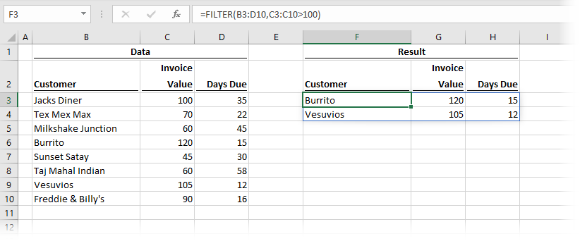
The formula in cell F3 is:
=FILTER(B3:D10,C3:C10>100)This single formula is returning 2 rows and 3 columns of data where the values in C3-C10 are higher than 100.
Example 2 – #CALC! error caused by the FILTER function
The screenshot below displays what happens when the result of the FILTER function has zero results; we get the #CALC! error.
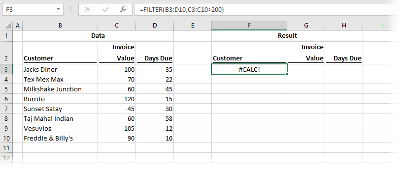
The formula in cell F3 is:
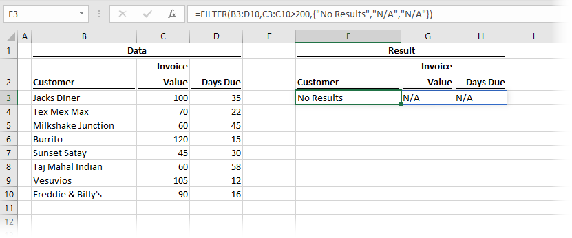
=FILTER(B3:D10,C3:C10>200)As no rows meet the criteria of Invoice Value being higher than 200, the FILTER cannot return a value, so the #CALC! error is displayed.
Thankfully, Microsoft has given us the if_empty argument, which displays a message if there are no rows returned.
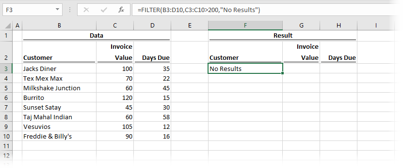
The formula in cell F3 is:
=FILTER(B3:D10,C3:C10>200,"No Results")In the screenshot above, No Results displays instead of the #CALC! error.
If we wanted to display a result in each column, we could include a constant array within the if_empty argument. The following shows n/a in the Invoice Value and Days Due columns.
=FILTER(B3:D10,C3:C10>200,{"No Results","n/a","n/a"})This formula would result in the following:
Example 3 – FILTER expands automatically when linked to a table
This example shows how the FILTER function responds when linked to an Excel table.
The FILTER is set to show items where Invoice Value is higher than 100. New records added to the Table which meet the criteria are automatically added to the spill range of the function. Amazing stuff!
Example 4 – Using FILTER with multiple criteria.
Example 4 shows how to apply FILTER with multiple criteria.
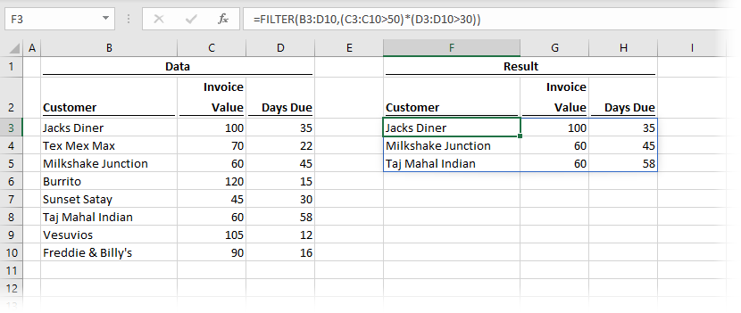
The formula in cell F3 is:
=FILTER(B3:D10,(C3:C10>50)*(D3:D10>30))For anybody who has used the SUMPRODUCT function, this method of applying multiple conditions will be familiar. Multiplication creates AND logic (i.e., all the criteria must be TRUE). The example above shows where the Invoice Value is greater than 50 and the Days Due is greater than 30.
Addition creates OR logic (i.e., any individual condition can be TRUE).
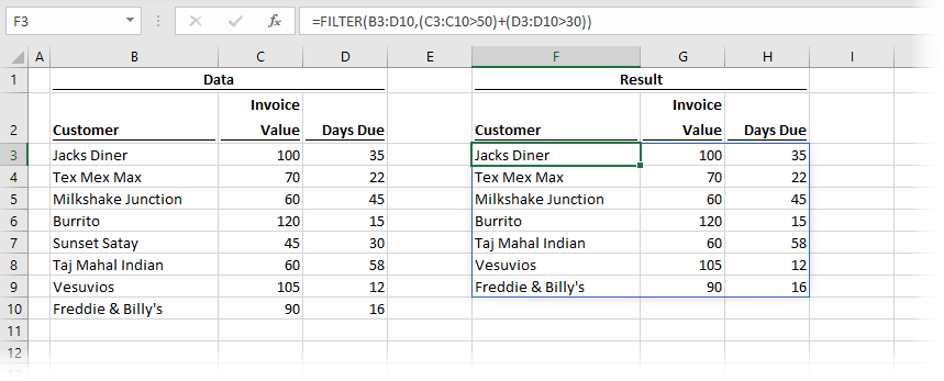
The formula in cell G3 is:
=FILTER(B3:D10,(C3:C10>50)+(D3:D10>30))The example above shows where the Invoice Value is greater than 50 or the Days Due is greater than 30.
Example 5 – Using FILTER for dependent dynamic drop-down lists
Drop-down lists are a data validation technique. Dependent drop-down lists are an advanced technique where the lists change depending on the result of another cell. For example, if the first drop-down list displays country names, the second drop-down list should only display cities that exist in that country. In Excel 2019 and before there are only tedious methods to achieve this effect, but the new FILTER function makes this super easy.
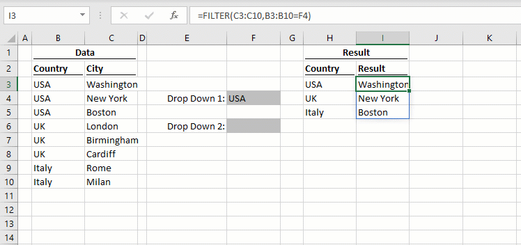
The formula in cell H3 is:
=UNIQUE(B3:B10)The UNIQUE function creates a unique list to populate the drop-down in cell F4.
The formula in cell I3 is:
=FILTER(C3:C10,B3:B10=F4)Depending on the value in cell F4, the values returned by the FILTER function change. The second drop-down in cell F6 changes dynamically based on the value in Cell F4.
Example 6 – Using FILTER with other functions
In this final example, FILTER is nested inside the SORT function.
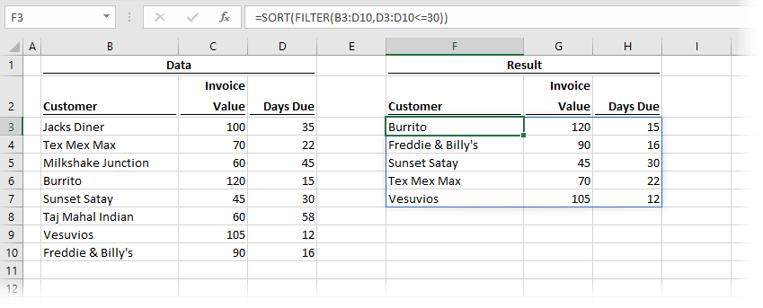
The formula in cell F3 is:
=SORT(FILTER(B3:D10,D3:D10<=30))First, the FILTER function returns the cells based on the Days Due being less than or equal to 30. The SORT function then puts the Customers into ascending alphabetical order.
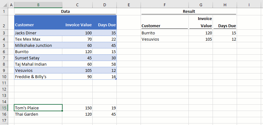
Example 7 – Using FILTER to show matching items from a list
How can we match a list of items that could have an unknown size? We can’t keep updating our FILTER function by adding and removing criteria. And, if we had a lot of items to match, it would soon become unmanageable. So, let’s see how we can solve this.
In the example below, the formula in cell H3 returns only the customers listed in F3:F4.
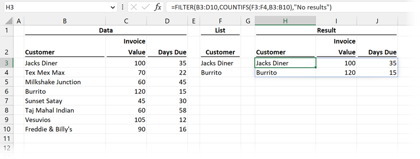
The formula in cell H3 is:
=FILTER(B3:D10,COUNTIFS(F3:F4,B3:B10),"No results")The COUNTIFS function returns a positive number if the item exists in both the data and the list, or zero if it exists in only one. Since positive numbers are always TRUE and zeros are always FALSE, this provides the TRUE/FALSE logic required for the FILTER function to return only the matching items.
NOTE: If the list starting in F3 were generated by another array formula, or by Power Query this solution would be completely dynamic (that is outside the scope of the current post, so we have used static ranges for this example).
Example 8 – Simulating wildcard search with FILTER
The FILTER function does not allow wildcard characters in the criteria. However, by using a combination of SEARCH and ISNUMBER we can simulate a similar effect.
In the example below, the formula in cell H3 returns only the items where the customer name contains the letters in cell F3.
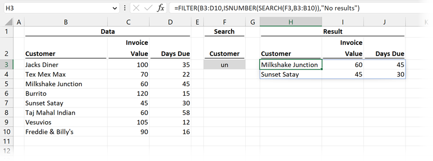
The formula in cell H3 is:
=FILTER(B3:D10,ISNUMBER(SEARCH(F3,B3:B10)),"No results")SEARCH returns a number if the search term in cell F3 is found in each value in B3-B10.
ISNUMBER returns TRUE or FALSE for each value depending on if SEARCH returns a number. This TRUE/FALSE value provides the logic needed by FILTER to return the matching items.
In this scenario only, Milkshake Junction and Sunset Satay contain un as a substring, therefore only these customers are returned.
Want to learn more?
There is a lot to learn about dynamic arrays and the new functions. Check out my other posts here to learn more:
- Introduction to dynamic arrays – learn how the excel calculation engine has changed.
- UNIQUE – to list the unique values in a range
- SORT – to sort the values in a range
- SORTBY – to sort values based on the order of other values
- FILTER – to return only the values which meet specific criteria
- SEQUENCE – to return a sequence of numbers
- RANDARRAY – to return an array of random numbers
- Using dynamic arrays with other Excel features – learn to use dynamic arrays with charts, PivotTables, pictures etc.
- Advanced dynamic array formula techniques – learn the advanced techniques for managing dynamic arrays

About the author
Hey, I’m Mark, and I run Excel Off The Grid.
My parents tell me that at the age of 7 I declared I was going to become a qualified accountant. I was either psychic or had no imagination, as that is exactly what happened. However, it wasn’t until I was 35 that my journey really began.
In 2015, I started a new job, for which I was regularly working after 10pm. As a result, I rarely saw my children during the week. So, I started searching for the secrets to automating Excel. I discovered that by building a small number of simple tools, I could combine them together in different ways to automate nearly all my regular tasks. This meant I could work less hours (and I got pay raises!). Today, I teach these techniques to other professionals in our training program so they too can spend less time at work (and more time with their children and doing the things they love).
Do you need help adapting this post to your needs?
I’m guessing the examples in this post don’t exactly match your situation. We all use Excel differently, so it’s impossible to write a post that will meet everybody’s needs. By taking the time to understand the techniques and principles in this post (and elsewhere on this site), you should be able to adapt it to your needs.
But, if you’re still struggling you should:
- Read other blogs, or watch YouTube videos on the same topic. You will benefit much more by discovering your own solutions.
- Ask the ‘Excel Ninja’ in your office. It’s amazing what things other people know.
- Ask a question in a forum like Mr Excel, or the Microsoft Answers Community. Remember, the people on these forums are generally giving their time for free. So take care to craft your question, make sure it’s clear and concise. List all the things you’ve tried, and provide screenshots, code segments and example workbooks.
- Use Excel Rescue, who are my consultancy partner. They help by providing solutions to smaller Excel problems.
What next?
Don’t go yet, there is plenty more to learn on Excel Off The Grid. Check out the latest posts:

The FILTER function in Excel is a very useful and frequently used function, that you will likely find the need for in many situations. Note that the FILTER function is only available in Microsoft Office 365, and Microsoft Office Online.
To filter by using the FILTER function in Excel, follow these steps:
- Type =FILTER( to begin your filter formula
- Type the address for the range of cells that contains the data that you want to filter, such as B1:C50
- Type a comma, and then type the condition for the filter, such as C3:C50>3 (To set a condition, first type the address of the «criteria column» such as B1:B, then type an operator symbol such as greater than (>), and then type the criteria, such as the number 3.
- Type a closing parenthesis and then press enter on the keyboard. Your entire formula will look like this: =FILTER(B1:C50,C1:C50>3)
In this article I will start with the basics of using the FILTER function (examples included), and then also show you some more involved ways of using the FILTER function. This article focuses specifically on the FILTER function that is typed into the spreadsheet cells as a formula, and not the filter command available from the toolbar and pop-up menus.
Using the FILTER function in Excel is almost the same as using it in Google Sheets, but there are slight differences between the two. Click here to read the Google Sheets version of this article
Here are the Excel Filters formulas:
Filter by a number
- =FILTER(A3:B12, B3:B12>0.7)
Filter by a cell value
- =FILTER(A3:B12, B3:B12<F1)
Filter by a text string
- =FILTER(A3:B12, B3:B12=»Late»)
Filter where NOT equal to
- =FILTER(A3:E1000, B3:B1000<>»Bob»)
Filter by date
- =FILTER(A3:C12,C3:C12<G1) (Date entered in cell G1)
- =FILTER(A3:C12,C3:C12<DATE(2019,6,1))
Filter by multiple conditions
- =FILTER(A3:C12,(B3:B12=»Late»)*(C3:C12=»Active»)) (AND logic)
- =FILTER(A3:C12, (B3:B12=»Late»)+(C3:C12=»Active»)) (OR logic)
Filter from another sheet
- =FILTER(‘Sheet Name’!A3:B12,’Sheet Name’!B3:B12=»Full Time»)
=FILTER(A3:B12, B3:B12=F1)
(Copy/Paste the formula above into your sheet and modify as needed)
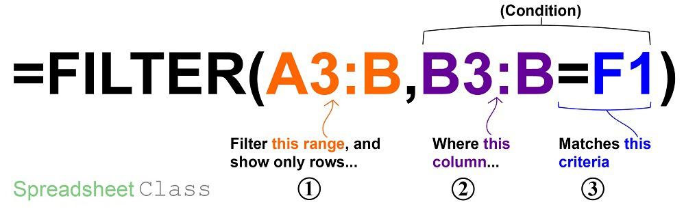
The FILTER function in Excel allows you to filter a range of data by a specified condition, so that a new set of data will be displayed which only shows the rows/columns from the original data set that meets the criteria/condition set in the formula.
Excel description for FILTER function:
Syntax:
=FILTER(array,include,[if_empty])Formula summary: “The FILTER function filters an array based on a Boolean (True/False) array.”
array (Required): The array, or range to filter
include (Required): A Boolean array whose height or width is the same as the array
[if_empty] (Optional): The value to return if all values in the included array are empty (filter returns nothing)
The source range that you want to filter, can be a single column or multiple columns.
The range that is used to check against the criteria that you set, must be a single column (later I will show you how to filter by multiple conditions, but don’t worry about that for now).
The criteria that set in the condition can be manually typed into the formula as a number or text, or it can also be a cell reference.
*Note that the source range and the single column range for the condition, must be the same size (must contain the same number of rows), or the cell will display an error.
Filtering by a single condition in Excel
First let’s go over using the FILTER function in Excel in its simplest form, with a single condition/criteria.
I will show you how to filter by a number, a cell value, a text string, a date… and I will also show you how to use varying «operators» (Less than, Equal to, etc…) in the filter condition.
Part 1: How to filter by a number
In this first example on how to use the filter function in Excel, the scenario is that we have a list of students and their grades, and that we want to make a filtered list of only students who have a perfect grade.
The task: Show a list of students and their scores, but only those that have a perfect grade
The logic: Filter the range A3:B12, where the column B3:B12 is greater than 0.7 (70%)
The formula: The formula below, is entered in the blue cell (D3), for this example
=FILTER(A3:B12, B3:B12>0.7)
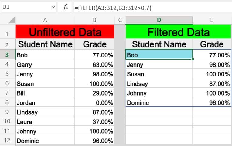
Operators that can be used in the FILTER function:
In this example we are using the operator «=» (Equal To) for the filter condition/criteria, but you can also use any of the following:
«=» (Equals)
«>» (Greater than)
«<» (Less than)
«<>» (Not equal to)
«>=» (Greater than or equal to)
«<=» (Less than or equal to)
Part 2: How to filter by a cell value in Excel
In this example, we want to achieve the same goal as discussed above, but rather than typing the condition that we want to filter by directly into the formula, we are using a cell reference.
When you filter by a cell value in Excel, your sheet will be setup so that you can change the value in the cell at any time, which will automatically update the value that the filter criteria it attached to.
In this example, you will notice that instead of directly typing the number “0.9” into the formula itself, the filter criteria is set as cell G1, where the “0.9” value is entered.
The task: Show a list of students and their scores, but only those that have a score below 90%
The logic: Filter the range A3:B12, where B3:B12 is less than the value that is entered in the cell F1 (0.9)
The formula: The formula below, is entered in the blue cell (D3), for this example
=FILTER(A3:B12, B3:B12<F1)
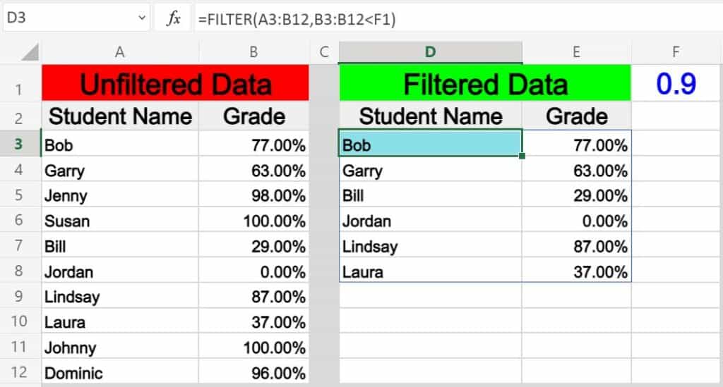
Part 3: How to filter by text in Excel
In this example, we are going to use a text string as the criteria for the filter formula. This is very similar to using a number, except that you must put the text that you want to filter by inside of quotation marks.
In this scenario we are filtering a list that shows customers and their payment status, and we want to display only customers that have a payment status of “Late”.
The task: Show a list of customers who are past due on their payments
The logic: Filter the range A3:B12, where B3:B12 equals the text, “Late”
The formula: The formula below, is entered in the blue cell (D3), for this example
=FILTER(A3:B12, B3:B12=»Late»)
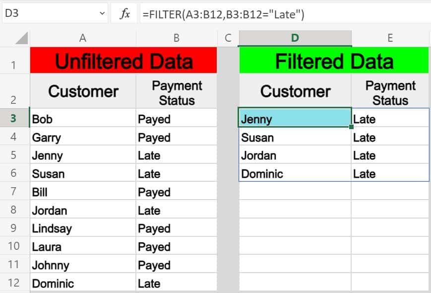
Part 4: Using NOT EQUAL TO in the Excel FILTER function
Now that you have got a basic understanding of how to use the filter function in Excel, here is another example of filtering by a string of text, but in this example we will use the «not equal» operator (<>), so that you can learn how to filter a range and output data that is NOT equal to criteria that you specify.
In this example we will also use a larger data set to demonstrate a more extensive application of the FILTER function in the real world.
You may be surprised at how often a situation comes up when you need to filter data where it is “not equal to” a certain number or piece of text that you specify.
In this example let’s say that we have a report/spreadsheet that shows data from sales calls that occur at your company, and we want to filter the data so that a specified sales rep (Bob) is NOT included in the filter output.
The task: Show sales call data for all sales reps, except Bob
The logic: Filter the range A2:E1000, where B2:B1000 DOES NOT equal the text, “Bob”
The formula: The formula below, is entered in the blue cell (G3), for this example
=FILTER(A3:E1000, B3:B1000<>»Bob»)
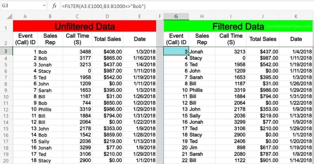
Notice that the filtered data on the right side of the image above does not contain any of the rows/calls that Bob was involved in.
Part 4: How to filter by date in Excel
Filtering by a date in Excel can be done in a couple of ways, which I will show you below. If you try to type a date into the FILTER function like you normally would type into a cell… the formula will not work correctly.
So you can either type the date that you want to filter by into a cell, and then use that cell as a reference in your formula… or you can use the DATE function.
When filtering by date you can use the same operators (>, <, =, etc…) as in other FILTER function applications. In Excel each different day/date is simply a number that is put into a special visual format. For example, in Excel, the date «06/01/2019» is simply the number «43,617», but displayed in date format. When you add one day to the date, this number increments by one each time… i.e «43,618» «43,619» «43,620»
So, one date can be considered to be «greater than» another date, if it is further in the future. Conversely, one date can be said to be «less than» another date, if it is further in the past.
In this first example we will filter by a date by using a cell reference. This is similar to the example we went over in part 2, but in this example instead of working with percentages, we are dealing with dates.
Let’s say that we want to filter a list of students, their test scores, and the dates that the tests were completed… and we want to show only tests that were taken before June (06/01/2019).
Filter by date in Excel example 1:
The task: Show only tests that were taken before June
The logic: Filter the range A3:C12, where C3:C12 is less than the date that is entered in cell G1 (06/01/2019)
The formula: The formula below, is entered in the blue cell (E3), for this example
=FILTER(A3:C12,C3:C12<G1)
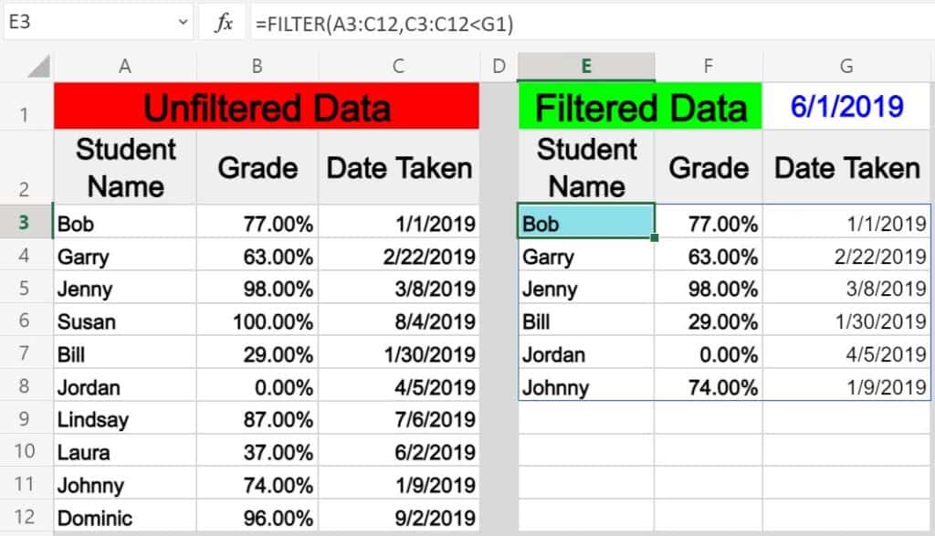
Filter by date in Excel example 2:
In this second example on filtering by date in Excel we are using the same data as above, and trying to achieve the same results… but instead of using a cell reference, we will use the DATE function so that you can type enter the date directly into the FILTER function.
When using the DATE function to designate a certain date, you must first enter the year, then the month, and then the day… each separated by commas (shown below).
The task: Show only tests that were taken before June
The logic: Filter the range A3:C12, where C3:C12 is less than the date of (06/01/2019)
The formula: The formula below, is entered in the blue cell (E3), for this example
=FILTER(A3:C12,C3:C12<DATE(2019,6,1))
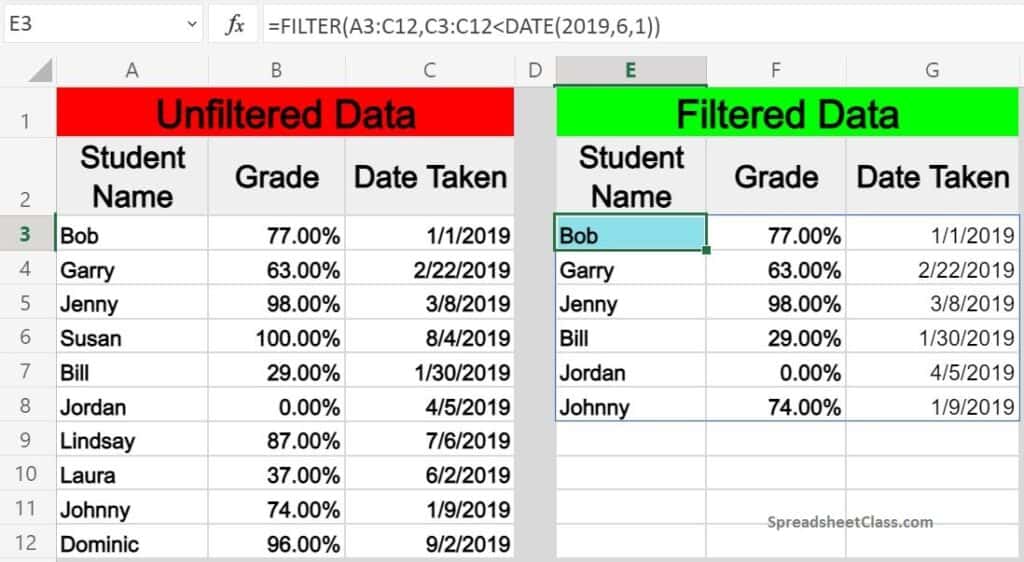
Filter by multiple conditions in Excel
When using the Excel FILTER function you may want to output a set of data that meets more than just one criteria. I will show you two ways to filter by multiple conditions in Excel, depending on the situation that you are in, and depending on how you want to formula to operate.
The normal way of adding another condition to your filter function, (as shown by the formula syntax in Excel), will allow you to set a second condition, where the first AND second condition must be met to be returned in filter output.
However I will also show you how to make a slight modification to the function so that you can choose to set a second condition where EITHER condition can be met to return/display in the filter function’s output/destination. (Separate the conditions with an asterisk to use AND logic, or separate the conditions with a plus sign to use AND logic.)
Part 5: Filtering by 2 conditions where BOTH MUST BE TRUE
In this example, we are going to filter a set of data, and only display rows where BOTH the first condition AND the second condition are met/true.
To use a second condition in this way (with AND logic), simply enter the second condition into the formula after the first condition, separated by an asterisk (*). Each condition must be inside of its own set of parenthesis (shown below).
When using the filter formula with multiple conditions like this, the columns that are referenced in each condition must be different.
In this scenario we want to filter a list that shows customers, their payment status, and their membership status… and to show only customers who have an active membership AND who are also late on their payment.
This will make sure that customers with an inactive membership who are still designated as being late on payment in the system… are not shown in the filter results, and not put on the list for being sent a «late payment» notice.
The task: Show a list of customers who are late on their payments, but only those with active memberships
The logic: Filter the range A3:C12, where B3:B12 equals the text “Late”, AND where C3:C12 equals the text “Active”
The formula: The formula below, is entered in the blue cell (E3), for this example
=FILTER(A3:C12,(B3:B12=»Late»)*(C3:C12=»Active»))
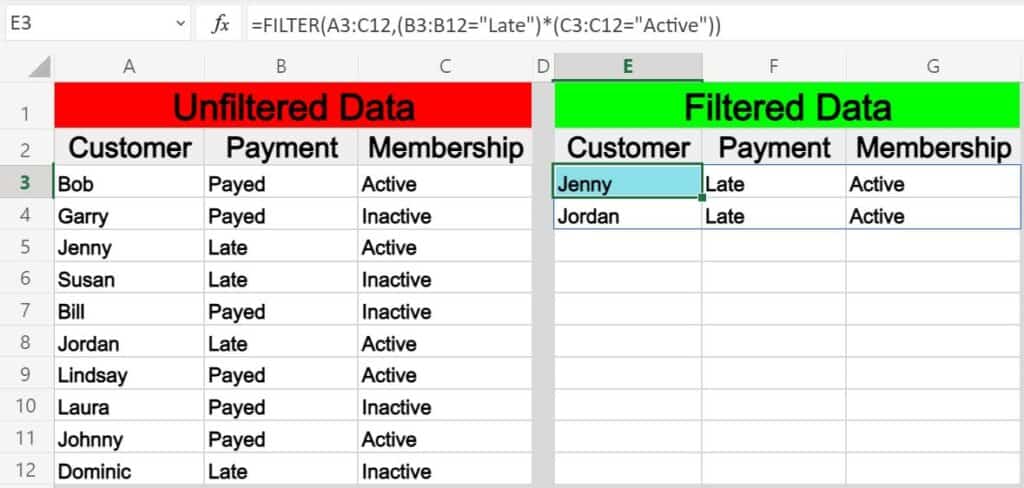
Part 6: Filtering by 2 conditions where EITHER ARE TRUE, not necessarily both
In this example we are going to filter a set of data and only display rows where EITHER the first condition OR the second condition are met/true.
To use a second condition in this way (with OR logic), simply enter the second condition into the formula after the first condition, separated by a plus sign. Each condition must be inside of its own set of parenthesis (shown below).
When using the FILTER formula in this way, you can choose criteria from the same or different columns.
In this scenario we want to filter the same customer data as shown in the previous example, but this time we want to show a list of customers who EITHER have an active membership OR who are late on their payment. This will give a list of customers who can be sent a notice for payment… including active members, or/also inactive members who are late on their final payment.
The task: Show a list of customers who are active members, and include customers who are late on payment even if they are not active members
The logic: Filter the range A3:C12, where B3:B12 equals the text “Late”, OR where C3:C12 equals the text “Active”
The formula: The formula below, is entered in the blue cell (E3), for this example
=FILTER(A3:C12, (B3:B12=»Late»)+(C3:C12=»Active»))
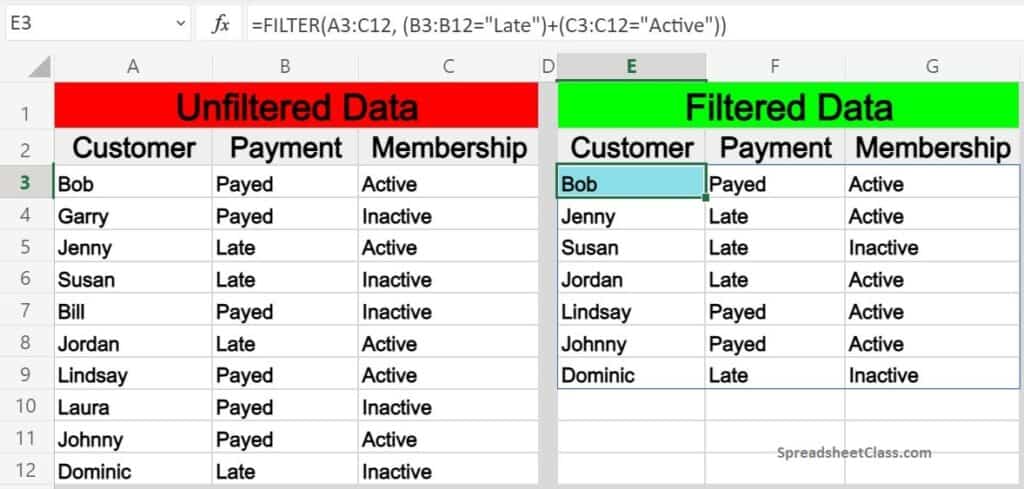
How to filter from another sheet in Excel
You may often find situations where you need to filter from another sheet in Excel, where your raw unfiltered data is on one tab, and your filter formula / filter output is on another tab.
This can be done by simply referring to a certain tab name when specifying the ranges in the filter. So where you would normally set a range like «A3:B», when referencing another sheet while filtering you specify the tab name by adding the tab name and an exclamation mark before the column/row portion of the range, like «TabName!A3:B»
However when the tab name has a space in it, it is necessary to use an apostrophe before and after the tab name, like ‘Tab Name’!A3:B.
Here is an example of how to filter data from another tab in Excel, where your filter formula will be on a different tab than the source range.
Let’s say that you have a list of employees and their schedule type (Full Time / Part Time) on one tab, and that you want to display a filtered list of full time employees on another tab.
The task: Filter the list of employees on the tab labeled «Filter List», and show a list of employees who have a full time schedule, on a separate tab
The logic: Filter the range ‘Filter List’!A3:B12, where the range ‘Filter List’!B3:B12 is equal to the text «Full Time»
The formula: The formula below, is entered in the blue cell (A3), for this example
=FILTER(‘Filter List’!A3:B12,’Filter List’!B3:B12=»Full Time»)
Here is a list of employees and their schedules, which is held on a tab labeled «Filter List»
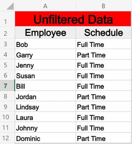
And here is a filtered list of employees who have full time schedules, where the filter formula and output data are held on a separate tab.
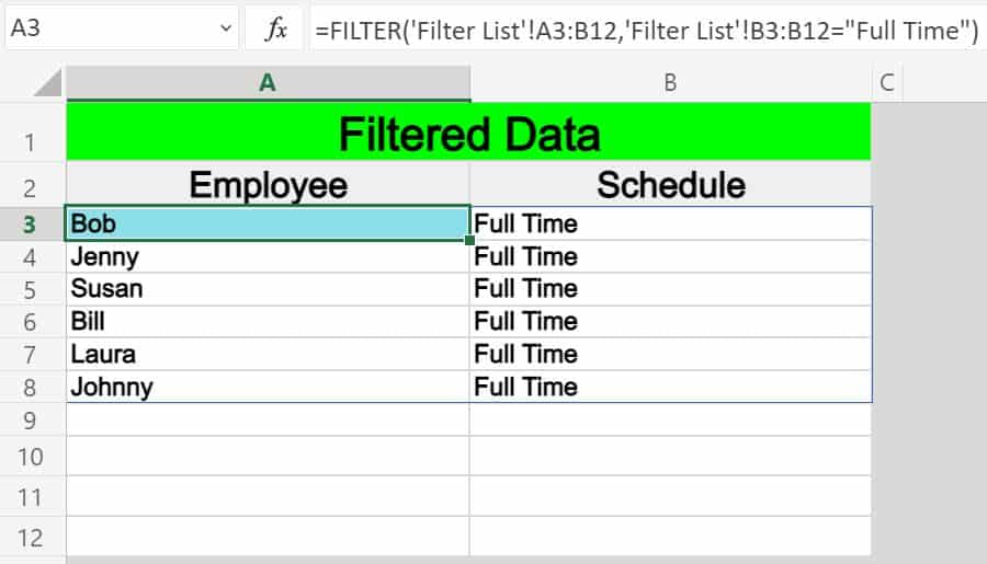
Pop Quiz: Test your knowledge
Answer the questions below about the Excel FILTER function, to refine your knowledge! Scroll to the very bottom to find the answers to the quiz.
Question #1
Which of the following formulas uses a «cell reference» in the filter condition?
- =FILTER(A1:D15, B1:B15<0.6)
- =FILTER(A2:C15, C2:C15=F1)
- =FILTER(A1:P25, G1:G25=»Yes»)
Question #2
Which of the following formulas uses the «Not Equal» operator?
- =FILTER(C1:T50, J1:J50>100)
- =FILTER(A1:B75, B1:B75=»No»)
- =FILTER(S1:Z100, T1:T100<>»True»)
Question #3
True or False: If the column(s) in the source range and the column in the filter condition are not the same size (if one has more rows than the other), the formula will not work, and will display an error.
- True
- False
Question #4
Which of the following formulas uses AND logic, where BOTH conditions must be met to satisfy the filter criteria?
- =FILTER(C1:F20, (F1:F20=»Yes»)+(E1:E20=»Active»))
- =FILTER(C1:F35, (F1:F35=»Yes»)*(E1:E35=»Active»))
Question #5
Which of the following formulas uses OR logic, where EITHER condition can be met to satisfy the filter criteria?
- =FILTER(A1:K10, (K1:K10=»Yes»)*(J1:J10=»Active»))
- =FILTER(A3:K33, (K3:K33=»Yes»)+(J3:J33=»Active»))
Answers to the questions above:
Question 1: 2
Question 2: 3
Question 3: 1
Question 4: 2
Question 5: 2

One of the most common things that I witness people (pros or amateurs / seniors or juniors) doing is applying filters to data. I mean it is so common that everyone knows it around. Agreed !
What I am going to share with you is 3 uncommon, incredibly smart ways of applying filters and not just filtering data but will also show you uncanny ways of automating filters
Method 1 – Auto Filter
This is a shortcut and will probably blow you away once you see how simple is it to use it.
Method 2 – Advanced Filter + Automation
Using advanced filter you can filter data for more complex conditions and even automate that using a tiny VB Code
Code for Pasting Filtered Data to another location
Sub My_Filter_Macro()
Range(“SalesData[#All]“).AdvancedFilter Action:=xlFilterCopy, _
CriteriaRange:=Range(“Condition[#All]“), CopyToRange:=Range(“Extract“), _
Unique:=False
End Sub
Code for Filtering data (without pasting it to another location)
Sub My_Filter_Same_Data()
Range(“SalesData[#All]“).AdvancedFilter Action:=xlFilterInPlace, CriteriaRange:= _
Range(“Condition[#All]“), Unique:=False
End Sub
To paste this code
- Open the VBA Window (Alt F11)
- In the menu click on Insert and then click on Module
- In the blank space, paste the code (make changes to the code if needed)
- Sweet..Done!
Method 3 – Filter Data using Slicers
You’ll feel like a King if you are working with Excel 2013 and above. Because you can use these nifty slicers to filter your data. Take a look
DOWNLOAD THE EXCEL FILE – with all methods + make sure to enable macros before you start toying with it
Create Dashboards using Slicers & Advanced Filter
- Create a Dashboard in 15 Mins – A small case where I’ll share simple tricks and hacks to make a quick dashboard using Filters Slicers and Formulas
- Advanced Filter Dashboard – Now since slicers work in Excel 2013 and above, you don’t have to feel disheartened. You can use advanced filter to create similar dashboard!
Topics that I write about…

Chandeep
Welcome to Goodly! My name is Chandeep.
On this blog I actively share my learning on practical use of Excel and Power BI. There is a ton of stuff that I have written in the last few years. I am sure you’ll like browsing around.
Please drop me a comment, in case you are interested in my training / consulting services. Thanks for being around
Chandeep
So you have thousands of rows of data in an Excel sheet, and you want to scan through the rows to find a pattern in the columns of the data.
You know you need an Excel filter to help you with that, but you don’t know how to go about it. Here, we’ll discuss all the best ways to filter your Excel sheet and show the data you need.
How to Filter in Excel
Assume you have an Excel sheet with three columns: age group, region, and the number of sales. In that case, an Excel filter can come in handy when you want to see your sales performance in a selected region, based on a particular age group.
Excel filters can also be useful when you want to create a smaller group before plotting your Excel data on a chart.
Let’s take a look at the following methods for filtering data in Excel.
How to Filter Based on Categories
Once you open your datasheet, on the Excel ribbon, click Data.
Next, locate the Sort & Filter group and click Filter. This puts a drop-down button on each column of your datasheet.
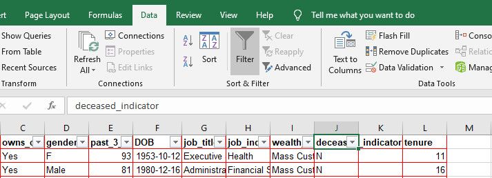
For instance, if your data has a gender column, which is a categorical variable, you can decide to filter your data to see only the female entries.
To do that, click the dropdown button on your categorical column of choice (gender in this case). In the menu that appears, untick everything by clicking the Select All box. Then select the values you want to filter your data by and click OK.
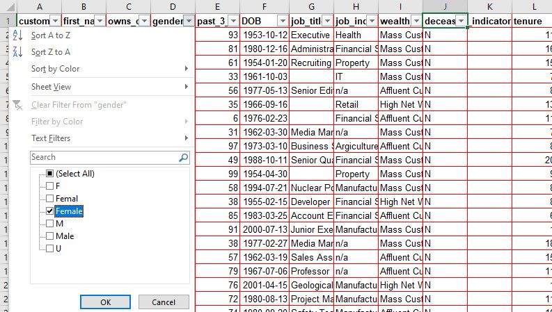
That operation filters the data based on the female listings, or whatever your categorical data of choice was. You can then check the lower-left corner of the Excel file to see the number of records on that particular filter.
While this option works for numbers as well, it’s usually inefficient and daunting. That’s because numbers can have a wider range of values. As such, ticking through the long list takes time.
How to Use Number Filters in Excel
Sometimes you might want to filter based on a particular range of numbers.
To use the number filter, click on Filter in the ribbon. Then click the dropdown button at the top of the column that contains the numbers you want to filter.
In the next menu, go to Number Filters and select your preferred choice from the options that pop up.
For instance, if you want to filter the column based on all numbers that are less than or equal to a certain number, from the Number Filters options, select Less than.
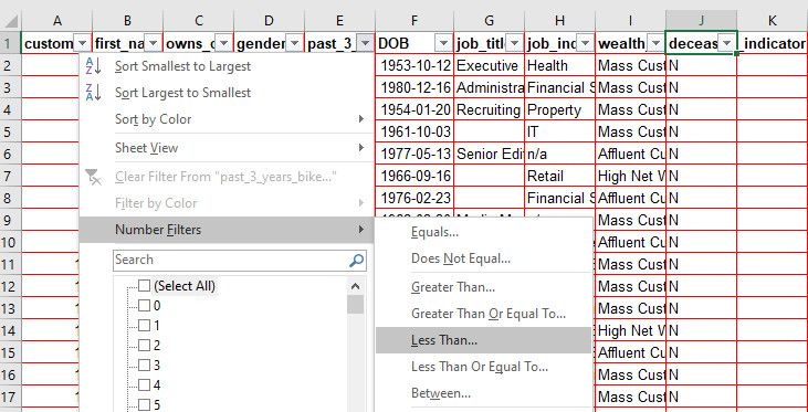
You can also use the And/Or section to add a second filter for your numbers.
Click OK when you’re done.
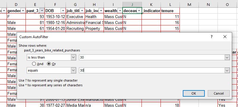
Lots of number-based filter options are available. You can play around with them to see how they work.
How to Use Advanced Filters in Excel
Excel’s advanced filter method offers a more flexible way of filtering data. With the advanced filter, you can separate your filtered result from the source data by pasting within the same sheet or in a new Excel sheet.
To use the advanced filter, create a new column on the right edge of your sheet. This new column is where you set your filtering criteria. You can leave a space between this criteria column and the last column of your source data to separate them if you want.
In the criteria column, type the exact name of the source data column you want to filter; a better alternative is to copy and paste the column heading to avoid mistakes.
In the next row, type the value you want to filter your data by for that column. For instance, if you want to see the data for all males in the gender column of the source data, type «male» beneath «gender» in your criteria section.
You can create multiple criteria columns to filter by if you like. To do that, copy the column names you want from the main data and paste them after your first criteria column.
Below each column heading, type in the data value you want to filter for.
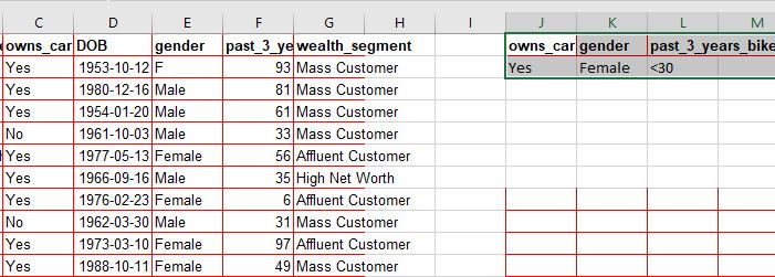
You can use Excel Boolean functions like less than (<) or greater than (>) as criteria for filtering numbers.
Once you’ve followed the process above, select Data in the Excel ribbon. Within the Sort & Filter group, click Advanced.
In the menu that opens, click the up arrow next to the List range field and choose which portion of your data you want to filter. Or ignore the List range field if you want to apply the filter to all your data.
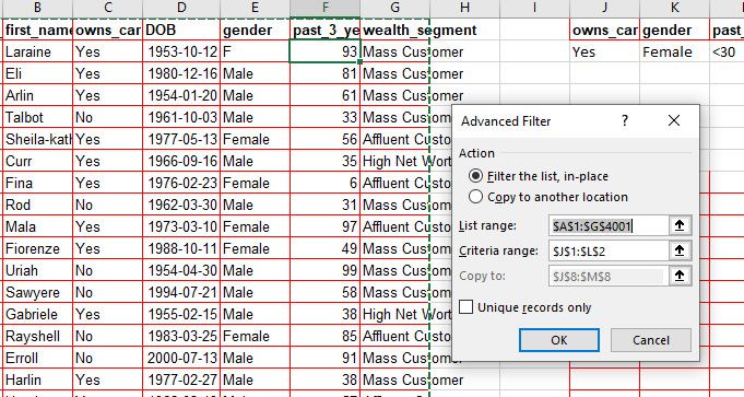
Next, place your cursor within the Criteria range field and highlight the criteria columns you created earlier: headings and values.
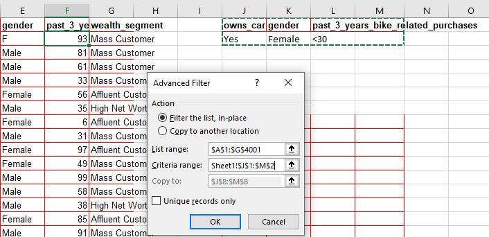
Click OK to apply the filter.
How to Paste the Filtered Results With the Advanced Filter Method
As we mentioned earlier, you can also use the advanced filter to separate your result and paste it somewhere else in the same sheet or in a new Excel sheet.
To do that, repeat the process above for filtering data with the advanced method. However, this time, in the Advanced Filter menu, select Copy to another location.
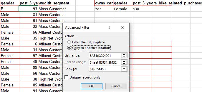
Next, place your cursor within the Copy to field and select any cell within your Excel sheet, then click OK.
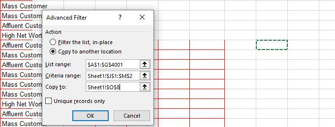
This operation copies the filtered result and pastes it at the selected location in your Excel sheet.
How to View the Filtered Result With Selected Columns in Excel
If you only want to view selected columns in the filtered data, highlight those column headings and copy them.
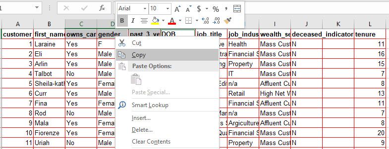
Next, paste the headings anywhere within the same sheet, where you want to see your filtered result.
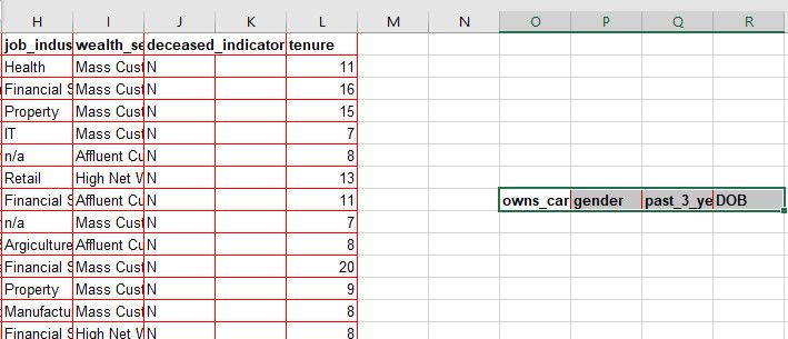
Repeat the process above for separating filtered results with the advanced filter method. But this time, once you get to the Copy to field, highlight the headings you pasted.
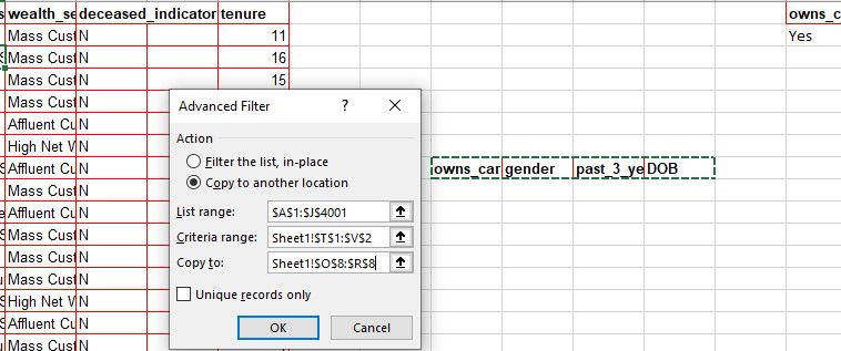
Then click OK to view the filtered result beneath these headings.
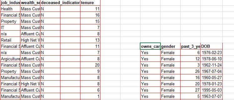
How to Use Advanced Filters to Paste the Filtered Result Into a New Excel Sheet
If you want to paste the resulting data into a new sheet, click on the Add (+) button at the lower-left corner of the Excel sheet to open a new sheet.
Click on any cell within the new sheet to activate it.
Select Data from the ribbon, then click on Advanced to make the Advanced Filter menu pop up. Select the Copy to another location option.
Place your cursor in the List range field and jump into the sheet that contains the source data. Then highlight the entire source data.
Next, place your cursor in the Criteria range field, highlight the criteria you created earlier in the source data sheet.
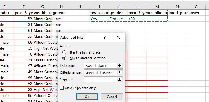
Select the Copy to field. Then select any cell on the new sheet again. Click OK to paste the filtered result to the new sheet.
Note: For this to work, ensure you activate the target sheet by clicking a cell within it first.
Get the Most Out of Excel Filters
While there are other options for filtering data, Excel is one of the most versatile productivity tools around. Although Excel filters can get a bit confusing, it’s easy once you master these tricks.
We’ve discussed the most common ways to filter data in Excel here, but there are even more advanced options available to if you play around with the advanced filter. When it comes to analyzing your filtered data, you might need the use of an Excel formula as well.