
Contents
- 1 How do you press enter in Excel and stay in the same cell?
- 2 How do you enter in an Excel cell?
- 3 Why can’t I hit Enter in Excel?
- 4 How do you press Enter?
- 5 What is Ctrl Enter in Excel?
- 6 How do you enter in the same column in Excel?
- 7 How do I enable the Enter key in Excel?
- 8 Where is Enter key on laptop?
- 9 What can I use instead of Enter key?
- 10 When you press Ctrl Enter you insert a?
- 11 How do I fill a column in Excel?
- 12 Why my Enter button is not working?
- 13 What is Ctrl +F?
- 14 What is the symbol for Enter key?
- 15 How do you press Enter without pressing enter?
- 16 How do you go to next line without pressing Enter?
- 17 Where is the enter button on HP laptop?
How do you press enter in Excel and stay in the same cell?
Stay in the same cell after pressing the Enter key with Shortcut Keys. In Excel, you can also use shortcut keys to solve this task. After entering the content, please press Ctrl + Enter keys together instead of just Enter key, and you can see the entered cell is still selected.
How do you enter in an Excel cell?
Click the location inside the cell where you want to break the line or insert a new line and press Alt+Enter.
Why can’t I hit Enter in Excel?
On the backstage screen, click “Options” in the list of items on the left. The “Excel Options” dialog box displays. Click “Advanced” in the list of items on the left. In the “Editing options” section, make sure the “After pressing Enter, move selection” check box is selected.
There are two Enter keys on a computer keyboard, one to the right of the main keyboard and the other on the bottom right corner of the numeric keypad. Keyboards and laptops without a numeric keypad only have one Enter key on the keyboard. Apple keyboards may have a Return key and an Enter key.
What is Ctrl Enter in Excel?
#2 – Ctrl+Enter to Fill All Selected Cells with the Same Data or Formula. When we are entering data or a formula in a cell, and have multiple cells selected, Ctrl+Enter will copy the data/formula to all of the selected cells.
How do you enter in the same column in Excel?
By default, when you press the “Enter” key on a spreadsheet, you will move the highlighted cell to the one below it. Use the Alt key to insert new lines into the same cell in a column.
How do I enable the Enter key in Excel?
To access this option, click File in the top left corner of your Excel document, and then click Options. The Excel Options dialog box will pop up and you will want to choose the Advanced tab. The top item listed allows you to change the behavior of the Enter key.
Where is Enter key on laptop?
The enter key is typically located to the right of the 3 and . keys on the lower right of the numeric keypad, while the return key is situated on the right edge of the main alphanumeric portion of the keyboard.
What can I use instead of Enter key?
You could replace it or use Ctrl+M instead of enter key. If the Enter key is not working, there is a high chance the Enter key is fine, but some other key is stuck, most likely ALT, CTRL, SHIFT, DEL, any key that would not show up doing something immediately.
When you press Ctrl Enter you insert a?
In a multi-line edit control on a dialog box, Ctrl + Enter inserts a carriage return into the edit control rather than executing the default button on the dialog box.
How do I fill a column in Excel?
Fill formulas into adjacent cells
- Select the cell with the formula and the adjacent cells you want to fill.
- Click Home > Fill, and choose either Down, Right, Up, or Left. Keyboard shortcut: You can also press Ctrl+D to fill the formula down in a column, or Ctrl+R to fill the formula to the right in a row.
Why my Enter button is not working?
The Enter key may not work if you are using the wrong keyboard driver or it’s out of date. To fix it, you can try reinstalling the keyboard driver with Device Manager. 1) On your keyboard, press the Windows logo key + R at the same time, type devmgmt. msc and click OK to open Device Manager.
What is Ctrl +F?
Updated: 12/31/2020 by Computer Hope. Alternatively known as Control+F and C-f, Ctrl+F is a keyboard shortcut most often used to open a find box to locate a specific character, word, or phrase in a document or web page.
What is the symbol for Enter key?
It normally has an arrow pointing down and left (⏎ or ↵), which is the symbol for carriage return. In contrast, the “Enter” key is commonly labelled with its name in plain text on generic PC keyboards, or with the symbol ⌤ (U+2324 up arrowhead between two horizontal bars) on many Apple Mac keyboards.
How do you press Enter without pressing enter?
You can use CTRL + J or CTRL + M as an alternative to Enter .
How do you go to next line without pressing Enter?
If you are searching for a way to move the cursor down a line without pressing the Enter key but still break the current line at that point, consider using a line break (Ctrl+Shift+L).
Where is the enter button on HP laptop?
The Enter (Return) key is basically the same on all laptops. The long arrow pointing to the left, on the right side of the keyboard is the return key.
How to Enter in Excel: Start a New Line in a Cell (2023)
Did you try pressing enter in excel expecting the cursor to move to the next line but met disappointment?
Yup, we have done the same. 😁
It simply happens because, unlike text editors, Excel does not let you move to the next line by pressing enter. Instead, it moves you to the next cell.
To help you with that, we are here to teach you a quick shortcut. You can insert a line break in excel on both Windows and Mac. You will also learn how to add a line break using the CONCATENATE function.
We have created a data set for you to practice. Download it here.
How to Start a New Line in a Cell
You can start a new line in Excel in less than 3 seconds – it’s so easy! Let’s consider an example.
Say you have a sentence.
Peter Piper picked a peck of pickled peppers. A peck of pickled peppers Peter Piper picked.

You want to divide the line into two separate parts:
(1) Peter Piper picked a peck of pickled peppers.
(2) A peck of pickled peppers Peter Piper picked.
In Excel, pressing the enter button will only move your cursor to the next cell. So to insert a line break in Excel:
- Double-click the selected cell.
- Place your cursor where you want to add a new line.
- Press enter.
You can also use the formula bar to start a new line in an Excel cell.
In our case, we want to insert the line break after the dot before the start of the second line.

- If you’re on Windows – press Alt + Enter to insert a line break.
- Otherwise, press CTRL + Option key + Return key to add a carriage return if you are on Mac.

The line break appears in the Excel cell. 😀
Pro Tip!
You can also add a line break after specific characters by using the Find and Replace feature. Select the cell and open the Find and Replace dialog box.
Enter the specific character in the find tab. Now, move to the replace tab and press CTRL + J. Click to replace all, and carriage returns appear at the specified positions.
How to Add Multiple Lines in a Cell
Adding multiple lines in Excel is no big deal. You can add more than one line in a single cell.
Say you have this sentence.
Peter Piper picked a peck of pickled peppers. A peck of pickled peppers Peter Piper picked. If Peter Piper picked a peck of pickled peppers?

And you want to break it into three parts like
(1) Peter Piper picked a peck of pickled peppers.
(2) A peck of pickled peppers Peter Piper picked.
(3) If Peter Piper picked a peck of pickled peppers?
It’s easy.
- Select the positions where you want to insert multiple lines.

- Press the Alt key + Enter to start a new line. You can also add spacing in selected cells – simply press the key combination twice.

Multiple line breaks appear in the selected cell.
Insert Line Breaks with CONCATENATE
Among Excel’s wide range of functions is the CONCATENATE function. It is a text-combining function and is represented by &.
Usually, it is written in one of these two ways:
- =CONCAT(text1, text2, [text3],..)
- =text1 & text2 & text3 &… textN
Let’s use the previous sentence as an example here. Say you want the following two phrases to be combined into one cell.
(1) Peter Piper picked a peck of pickled peppers.
(2) A peck of pickled peppers Peter Piper picked.

Enter appropriate arguments in the formula. Since our text is in cells A2 and A3, we will use the following formula:
=A2 & ” ” & A3
Upon exiting the edit mode, Microsoft Excel will show the sentence in a single line.

But that’s not what we wanted. Why didn’t the line break appear? 🤔
That’s because the Enter keyboard shortcut does not work with formulas. Excel needs the CHAR function for inserting line breaks with functions.
So, to insert a line break:
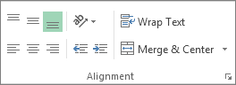
- We will enable wrap text feature from the Home Tab for the selected cell. It is under the alignment group.

Once the toggle button is switched on for the selected cell, we will add the CHAR function. Each OS has a special character code, and the code for a line break in Windows is 10 and 13 for Mac.
- Add CHAR(10) in the formula in place of ” ” to add a line break
=A2 & CHAR(10) & A3.

The line feed appears in the Excel cell.
You can also use the TEXTJOIN function in place of CONCATENATE – they both serve the same purpose.
Show New Lines with Wrap Text
Wrap text lets you easily insert line breaks between text strings in the same cell. Simply select the cell with text inside and click the wrap text button from the Home Tab.
As evident from the name, the wrap text feature ‘wraps’ the text around a worksheet cell. It adjusts the text and adds line breaks automatically to autofit the column width.
For instance, the first line in this worksheet exceeds the location inside the column. As it occupies the next several cells.

To adjust it, we will use wrap text to limit the line in an Excel cell.
- Select the cell.
- Adjust the row height.
- Enable the wrap text feature.
The text will now look something like this:

You can do the same for the next row and other multiple cells.
That’s it – Now what?
This article taught us how to enter single and multiple line breaks in a cell. We also saw how to use the wrap text feature in Excel and a quick trick to add a new line with formulas.
Although these shortcuts come in handy while working in Excel, they constitute only a small part of this gigantic spreadsheet software.
Excel has so much more to offer, like the basic VLOOKUP, IF, and SUMIF functions that you must learn.
Enroll in my 30-minute free email course that can help you master these functions (and more!). 😀
Kasper Langmann2023-02-23T11:44:22+00:00
Page load link
Содержание
- Start a new line of text inside a cell in Excel
- Need more help?
- How To Press Enter In An Excel Cell?
- How do you press enter in Excel and stay in the same cell?
- How do I enter multiple lines in an Excel cell?
- Which command is used to enter a line in a cell in Excel?
- Can’t hit Enter in Excel cell?
- When you press the Enter key the cell pointer?
- How do you press Enter?
- How do you insert multiple lines in one cell?
- How do you show all writing in an Excel cell?
- What is Ctrl Enter in Excel?
- How do you put a dot point in Excel?
- What can I use instead of Enter key?
- How do you press Enter without pressing enter?
- What is shortcut for Enter key?
- When you type data in a cell and press Enter?
- Which commands is used to display text in a cell in multiple lines?
- How do I get cells to show all text in sheets?
- What does Ctrl Alt Enter do?
- How to Start a New Line in Excel Cell (Keyboard Shortcut + Formula)
- Start a New Line in Excel Cell – Keyboard Shortcut
- Start a New Line in Excel Cell Using Formula
- Using TextJoin Formula
- Using Concatenate Formula
- New Line in an Excel Cell
- Insert a New Line in an Excel Cell
- Top 3 Ways to Insert a New Line in a Cell of Excel
- #1 – Using the Shortcut Keys “Alt+Enter”
- #2–Using the “CHAR(10)” Formula of Excel
- #3–Using the Named Formula [CHAR(10)]
- Frequently Asked Questions
- Recommended Articles
Start a new line of text inside a cell in Excel
To start a new line of text or add spacing between lines or paragraphs of text in a worksheet cell, press Alt+Enter to insert a line break.
Double-click the cell in which you want to insert a line break.
Click the location inside the selected cell where you want to break the line.
Press Alt+Enter to insert the line break.
To start a new line of text or add spacing between lines or paragraphs of text in a worksheet cell, press CONTROL + OPTION + RETURN to insert a line break.
Double-click the cell in which you want to insert a line break.
Click the location inside the selected cell where you want to break the line.
Press CONTROL+OPTION+RETURN to insert the line break.
To start a new line of text or add spacing between lines or paragraphs of text in a worksheet cell, press Alt+Enter to insert a line break.
Double-click the cell in which you want to insert a line break (or select the cell and then press F2).
Click the location inside the selected cell where you want to break the line.
Press Alt+Enter to insert the line break.
Double-tap within the cell.
Tap the place where you want a line break, and then tap the blue cursor.

Tap New Line in the contextual menu.
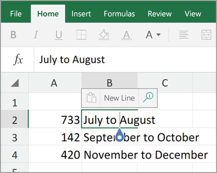
Note: You cannot start a new line of text in Excel for iPhone.
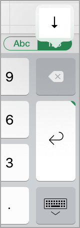
Tap the keyboard toggle button to open the numeric keyboard.

Press and hold the return key to view the line break key, and then drag your finger to that key.
Need more help?
You can always ask an expert in the Excel Tech Community or get support in the Answers community.
Источник
How To Press Enter In An Excel Cell?
Excel 2016 Click the location inside the cell where you want to break the line or insert a new line and press Alt+Enter.
How do you press enter in Excel and stay in the same cell?
Stay in the same cell after pressing the Enter key with Shortcut Keys. In Excel, you can also use shortcut keys to solve this task. After entering the content, please press Ctrl + Enter keys together instead of just Enter key, and you can see the entered cell is still selected.
How do I enter multiple lines in an Excel cell?
5 steps to better looking data
- Click on the cell where you need to enter multiple lines of text.
- Type the first line.
- Press Alt + Enter to add another line to the cell. Tip.
- Type the next line of text you would like in the cell.
- Press Enter to finish up.
Which command is used to enter a line in a cell in Excel?
To start a new line in an Excel cell, you can use the following keyboard shortcut:
- For Windows – ALT + Enter.
- For Mac – Control + Option + Enter.
Can’t hit Enter in Excel cell?
Cell Movement After Enter
- Display the Excel Options dialog box.
- At the left of the dialog box click Advanced.
- Make sure the After Pressing Enter Move Selection check box is selected.
- Use the Direction drop-down list to specify the direction that Excel should move.
- Click OK.
When you press the Enter key the cell pointer?
By default, in Microsoft Excel, when you press the Enter key, it moves the cell pointer one cell down.
How do you press Enter?
Alternatively known as a Return key, with a keyboard, the Enter key sends the cursor to the beginning of the next line or executes a command or operation. Most full-sized PC keyboards have two Enter keys; one above the right Shift key and another on the bottom right of the numeric keypad.
How do you insert multiple lines in one cell?
If you want to paste all the contents into one cell, you can use this method.
- Press the shortcut key “Ctrl + C” on the keyboard.
- And then switch to the Excel worksheet.
- Now double click the target cell in the worksheet.
- After that, press the shortcut key “Ctrl + V” on the keyboard.
How do you show all writing in an Excel cell?
Select the cells that you want to display all contents, and click Home > Wrap Text. Then the selected cells will be expanded to show all contents.
What is Ctrl Enter in Excel?
#2 – Ctrl+Enter to Fill All Selected Cells with the Same Data or Formula. When we are entering data or a formula in a cell, and have multiple cells selected, Ctrl+Enter will copy the data/formula to all of the selected cells.
How do you put a dot point in Excel?
How to Add Bullet Points in Excel
- Select the cell in which you want to insert the bullet.
- Either double click on the cell or press F2 – to get into edit mode.
- Hold the ALT key, press 7 or 9, leave the ALT key.
- As soon as you leave the ALT key, a bullet would appear.
What can I use instead of Enter key?
You could replace it or use Ctrl+M instead of enter key. If the Enter key is not working, there is a high chance the Enter key is fine, but some other key is stuck, most likely ALT, CTRL, SHIFT, DEL, any key that would not show up doing something immediately.
How do you press Enter without pressing enter?
You can use CTRL + J or CTRL + M as an alternative to Enter .
What is shortcut for Enter key?
Windows Laptops:
Hold down the “fn” key and press the ‘num lk’ key. On some laptops this key is the same as the ‘end’ key. Once the num lock function has been enabled, the Return key will function as an Enter key.
When you type data in a cell and press Enter?
By default when typing data or a formula into a cell and pressing enter, the active cell cursor will move down one cell. You don’t have to be stuck with this if you don’t want it though. You can also have it go up, left, right or not move at all if you want.
Which commands is used to display text in a cell in multiple lines?
You can put multiple lines in a cell with pressing Alt + Enter keys simultaneously while entering texts. Pressing the Alt + Enter keys simultaneously helps you separate texts with different lines in one cell.
How do I get cells to show all text in sheets?
How to Wrap Text in Google Sheets
- Select the cells you want to set to wrap.
- Click Format.
- Select Text wrapping.
- Select Wrap.
What does Ctrl Alt Enter do?
Popular programs using this shortcut
You can apply different paragraph styles to the left and right of the style separator. That can be useful for references. And you can also use it to limit the text that is included in the Table of Contents. PyCharm 2018.2 – Start a new line before the current one.
Источник
How to Start a New Line in Excel Cell (Keyboard Shortcut + Formula)
Watch Video – Start a New Line in a Cell in Excel (Shortcut + Formula)
In this Excel tutorial, I will show you how to start a new line in an Excel cell.
You can start a new line in the same cell in Excel by using:
- A keyboard shortcut to manually force a line break.
- A formula to automatically enter a line break and force part of the text to start a new line in the same cell.
This Tutorial Covers:
Start a New Line in Excel Cell – Keyboard Shortcut
To start a new line in an Excel cell, you can use the following keyboard shortcut:
- For Windows – ALT + Enter.
- For Mac – Control + Option + Enter.
Here are the steps to start a new line in Excel Cell using the shortcut ALT + ENTER:
- Double click on the cell where you want to insert the line break (or press F2 key to get into the edit mode).
- Place the cursor where you want to insert the line break.
- Hold the ALT key and press the Enter key for Windows (for Mac – hold the Control and Option keys and hit the Enter key).

Start a New Line in Excel Cell Using Formula
While keyboard shortcut is fine when you are manually entering data and need a few line breaks.
But in case you need to combine cells and get a line break while combining these cells, you can use a formula to do this.
Using TextJoin Formula
If you’re using Excel 2019 or Office 365 (Windows or Mac), you can use the TEXTJOIN function to combine cells and insert a line break in the resulting data.
For example, suppose we have a dataset as shown below and you want to combine these cells to get the name and the address in the same cell (with each part in a separate line):

The following formula will do this:
At first, you may see the result as one single line that combines all the address parts (as shown below).

To make sure you have all the line breaks in between each part, make sure the wrap text feature is enabled.
To enable Wrap text, select the cells with the results, click on the Home tab, and within the alignment group, click on the ‘Wrap Text’ option.

Once you click on the Wrap Text option, you will see the resulting data as shown below (with each address element in a new line):

Using Concatenate Formula
If you’re using Excel 2016 or prior versions, you won’t have the TEXTJOIN formula available.
So you can use the good old CONCATENATE function (or the ampersand & character) to combine cells and get line break in between.
Again, considering you have the dataset as shown below that you want to combine and get a line break in between each cell:
For example, if I combine using the text in these cells using an ampersand (&), I would get something as shown below:

While this combines the text, this is not really the format that I want. You can try using the text wrap, but that wouldn’t work either.
If I am creating a mailing address out of this, I need the text from each cell to be in a new line in the same cell.
To insert a line break in this formula result, we need to use CHAR(10) along with the above formula.
CHAR(10) is a line feed in Windows, which means that it forces anything after it to go to a new line.
So to do this, use the below formula:
This formula would enter a line break in the formula result and you would see something as shown below:
IMPORTANT : For this to work, you need to wrap text in excel cells. To wrap text, go to Home –> Alignment –> Wrap Text. It is a toggle button.

Tip: If you are using MAC, use CHAR(13) instead of CHAR(10).
You may also like the following Excel Tutorial:
Источник
New Line in an Excel Cell


Insert a New Line in an Excel Cell
A new line in excel cell is inserted when one needs to move a string to the next line of the cell. To insert a new line, a line break must be added at the relevant place. A line break tells Excel to break the existing line and begin a new line (within the same cell) with the immediately following character. When line breaks are inserted in a cell, its content can be seen in multiple lines.
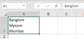
For example, in the following image, a line break has been inserted after the cities Bangalore and Mysore. So, a total of two line breaks have been inserted in cell A1. Notice that the three cities are in three different rows of the same cell.

Starting a new line in an excel cell ensures that the lengthy text strings are split into multiple lines. This improves the readability and lends a neat look to the worksheet. To obtain the right result after inserting line breaks, ensure that the wrap text feature of Excel is turned on.
Table of contents
Top 3 Ways to Insert a New Line in a Cell of Excel
The methods to start a new line in a cell of Excel are listed as follows:
- Shortcut keys “Alt+Enter”
- “CHAR(10)” formula of Excel
- Named formula [CHAR(10)]
Let us consider an example of each technique.
Note: The line feed (LF) and carriage return Carriage Return Carriage Return in excel cell is a way to shift to a new line within the same cell. This could be treated as a line breaker which fits in huge data in an organized manner within one cell. read more (CR) are two terms closely related to a line break. The LF moves the cursor to the next line within the cell. In contrast, a CR moves the cursor to the beginning (or the first position) of the same line. So, with a CR alone, the cursor does not move to the next line.
Every operating system considers a line break (LF or CR or a combination of CR and LF) differently. For instance, when a line break is inserted in the Windows operating system, both CR and LF (called CR+LF or CRLF) are inserted together.
The CRLF moves the cursor to the beginning of the next line. However, the “Alt+Enter” method inserts only line feeds in Excel. The ASCII (American Standard Code for Information Interchange) codes for LF and CR are 10 and 13 respectively.
In this article, the usage of code 10 has been shown in example #2. Further, this article uses the term line break in place of line feed and carriage return. Hence, consider all three (line break, line feed, and carriage return) to be the same in this article.
#1 – Using the Shortcut Keys “Alt+Enter”
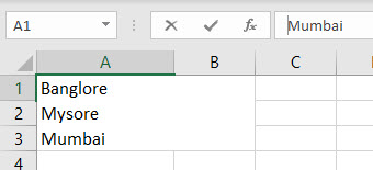
The following image shows the names of three cities of India in cell A1. We want to insert a line break after the first two cities of this cell. Use the keys “Alt+Enter” of Excel.

The steps to insert line breaks by using the keys “Alt+Enter” are listed as follows:
Step 1: Double-click inside cell A1. Next, move and bring the cursor immediately before the “M” of Mysore. To do this, either move the cursor with the arrow keys of the keyboard or click at the stated position with the left-click of the mouse.
The cursor is placed before Mysore because a line break needs to be inserted at this position.
Note: Alternatively, one can also place the cursor at the stated position in the formula bar.

Step 2: Press the keys “Alt+Enter.” For this shortcut to work, hold the “Alt” key while pressing the “Enter” key.
A new line is inserted before “Mysore,” as shown in the following image.

Step 3: Place the cursor before the “M” of Mumbai by using the left-click of the mouse. Press the keys “Alt+Enter,” the way they were pressed in the preceding step.
The name “Mumbai” shifts to a new line within the same cell of Excel. This is shown in the following image.
Step 4: Press the “Enter” key to exit the Edit mode. The following image shows the names of the three cities in multiple lines of a single cell (cell A1) of Excel. This result will be displayed only if the wrap text feature of Excel is turned on.
Notice that the formula bar (in the following image) shows a line break after Bangalore.
Note: The “wrap text” is a toggle button in the “alignment” group of the Home tab. It can also be accessed from the “alignment” tab of the “format cells” window. This window can be opened by pressing the shortcut “Ctrl+1.”
By default, the wrap text feature is turned on when a line break is inserted with the “Alt+Enter” method in Excel. To cross-check, keep cell A1 selected and notice that the “wrap text” button is automatically activated after inserting a line break with the shortcut keys.
If the wrap text button is turned off, the content of cell A1 will display in a single line. However, the line breaks will still be visible in the formula bar.
#2–Using the “CHAR(10)” Formula of Excel
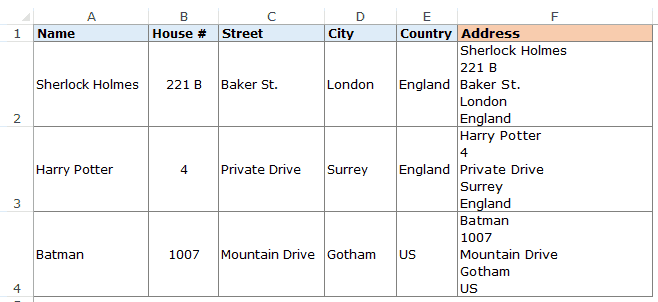
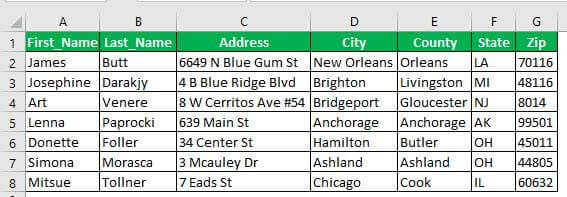
The following image shows the names and addresses of some people. The first and the last names have been split into columns A and B respectively. The address has been split into columns C to G. We want to perform the following tasks:
- Join the first and the last name to the full address of each person. For this, combine the strings of columns A and B with those of columns C to G. Use the ampersand (&) to join the stated strings. Ensure that a single space character precedes each string of the address.
- Insert a line break between the last name and the first character of the address. Use the CHAR function for inserting line breaks.
In the end, the complete name should be in one line, followed by the address in the subsequent lines of the cell. Further, use a single formula for performing the given tasks. Explain the formula used.
Step 1: Insert a new column to the right of the given dataset. We have inserted column H titled “full address.” This is shown in the following image.

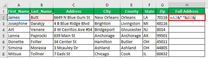
Step 2: Begin by combining the first and last names (of row 2) with the ampersand. To do this, type the following formula in cell H2.
This formula joins the first and the last names of cells A2 and B2 and also inserts a space between them. However, the formula is currently incomplete.
Step 3: Extend the preceding formula to include the CHAR function. Open this function by typing “CHAR,” followed by the opening parenthesis.
The opening of the CHAR function is shown in the following image.
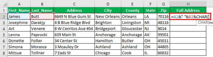
Step 4: Insert the number 10 within the CHAR function. The “CHAR(10)” formula inserts a line break in Excel.
Note: The syntax of the CHAR function is “CHAR(number).” This function returns a character when a number between 1 and 255 is entered. The character is returned from the character set of the user’s computer.
Earlier, the Windows operating system used the ASCII and the ANSI character sets, which have now been replaced by Unicode. The ASCII stands for American Standard Code for Information Interchange. The ANSI character set was created by the American National Standard Institute.
In contrast, the Macintosh operating system uses the Macintosh character set. So, the Macintosh users may use the formula “CHAR(13)” to insert a line break in Excel.
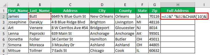
Step 5: Insert the cell references to be joined with the strings of cells A2 and B2. So, in cell H2, enter the following formula by excluding the beginning and ending double quotation marks.
Press the “Enter” key. The output appears in cell H2. The formula and the output are shown in the following image. The output is not fully visible as it is in a single line of cell H2 of Excel.

Explanation of the formula: The preceding formula joins the first and the last names (in cells A2 and B2) with the entire address of a person (in cells D2, E2, F2, and G2). The ampersand (&) is used to join.
Notice that, in the formula, a space character has been inserted preceding the strings of cells D2, E2, F2, and G2. This space character is inserted within double quotation marks (like “ ”). These spaces of the formula ensure that spaces are inserted as separators in the output. Moreover, the separators are inserted at exactly those places (in the output) where they have been entered in the formula.
However, no space is inserted between the strings of cells B2 and C2. Rather, the “CHAR(10)” has been used in place of a space. This is because the “CHAR(10)” moves the immediately following string (of cell C2) to the next line.
Step 6: Activate the wrap text feature of Excel to see the entire content of cell H2. So, select cell H2 and click the “wrap text” button in the “alignment” group of the Home tab.
The output is shown in the following image. The full name and the complete address are visible in cell H2. Not only the strings of cells A2 to G2 have been joined, but a line break has also been inserted after the name (James Butt). As a result, a legible output has been obtained in cell H2.
Note: When a line break is inserted by the CHAR function, the wrap text feature of Excel is not turned on by default. Rather, this feature needs to be enabled manually to see the impact of the line break.

Step 7: Drag the formula of cell H2 till cell H8 by using the fill handle. The fill handle is displayed at the bottom-right corner of cell H2.
The dragging of the fill handle and the outputs are shown in the following image. Hence, the names and addresses have been consolidated neatly in column H.
#3–Using the Named Formula [CHAR(10)]
Working on the dataset of example #2, we want to perform the following tasks:
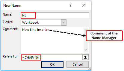
- Assign the name “NL” to the “CHAR(10)” formula. By doing this, “CHAR(10)” becomes a named formula.
- Add the comment “new line inserter” to the name “NL.”
- Show how to use the name “NL” (representing the named formula) in the ampersand and CHAR formula of example #2. Explain the formula thus used.
Use the “define name” property of Excel for the first two bullet points.
The steps to perform the given tasks by using the named formula are listed as follows:
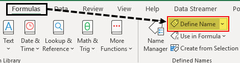
Step 1: Click “define name” from the “defined names” group of the Formulas tab. This option is shown in the following image.
Step 2: The “new name” window opens, as shown in the following image. Make the following insertions in this window:
- In the “name” box, enter the name “NL.”
- In the “scope” box, let the option “workbook” remain selected.
- In the “comment” box, enter the string “new line inserter.”
- In the “refers to” box, enter the formula “=CHAR(10).”
Ensure that the insertions of points “a,” “c,” and “d” are entered without the beginning and ending double quotation marks. Click “Ok” once the insertions are done.
Note 1: The name and the comment cannot exceed 255 characters in length. The name must begin with a letter, underscore (_) or backslash (). Further, the name should not consist of any space characters.
Step 3: Use “NL” in place of “CHAR(10)” in the following formula.
Press the “Enter” key. The outputs are shown in the following image.
Note: When the “N” of “NL” is typed in the formula, Excel shows the name (NL) as well as the comment (new line inserter) in a list of suggestions. To select “NL” from this list, just double-click it.

Explanation of the formula: The outputs of the preceding formula are the same as that of example #2 (in step 7). This is because other than the name “NL,” the formulas of the two examples (examples #2 and #3) are the same.
Since “CHAR(10)” has been named “NL,” we have used this name in the formula instead of the CHAR function. The “wrap text” feature has also been applied to cell H2. This is the reason its content has fitted into multiple lines of cell H2 of Excel.
Notice that using a different name for “CHAR(10)” has not impacted the result. Rather, using the name “NL” has made the preceding formula compact and understandable.
Note: In this example, “CHAR(10)” is considered a named formula. A named formula is one that has been assigned a name in Excel. Assigning a name (like “NL”) to a formula [like “CHAR(10)”] helps refer to the formula by its name.
So, every time one needs to use “CHAR(10)” in the formulas of the current workbook, one can use “NL” in its place. This is because the “scope” in the “new name” window has been set as “workbook.”
Frequently Asked Questions
Inserting a new line means moving the content of a cell to the next line. This allows one to break lengthy text strings and display their data in multiple lines of a single cell. The shortcuts for inserting a line break in Excel are stated as follows:
Windows operating system – The shortcut is “Alt+Enter.” For this shortcut to work, hold the “Alt” key while pressing the “Enter” key.
Macintosh operating system – The shortcut is “Control+Option+Return” (or “Control+Command+Return”). For this shortcut to work, hold the “Control” and the “Option” keys while pressing the “Return” key.
Note: Before using the preceding shortcuts, ensure that the cursor is placed where a line break needs to be inserted.
The CONCATENATE function joins the values of different cells in a single cell. Thereafter, the “CHAR(10)” inserts line breaks in the single output cell.
The CONCATENATE and CHAR formula for inserting a new line in Excel is stated as follows:
“CONCATENATE(cell1,CHAR(10),cell2,CHAR(10),cell3,CHAR(10)…)”
The steps for inserting a new line with the Find and Replace feature of Excel are listed as follows:
a. Select the cells in which a new line needs to be inserted.
b. Press the keys “Ctrl+H” to open the Replace tab of the Find and Replace window. Alternatively, click the “find & select” drop-down from the “editing” group of the Home tab. Then, select the “replace” option.
c. In the “find what” box, type the separator that separates the strings. For instance, if a comma separates the strings, type a comma. Likewise, if a space separates the strings, type a space.
d. In the “replace with” box, press the keys “Ctrl+J.” A small, blinking dot appears in this box.
e. Click “replace all.”
In the selected cells, all occurrences of the separator (typed in step “c”) will be replaced by line breaks.
Note: Use the Find and Replace feature for inserting line breaks when each selected cell contains at least one occurrence of the separator. At the same time, there is a need to replace all these occurrences with line breaks.
The formula to remove a line break from a cell is stated as follows:
“=SUBSTITUTE(cell1,CHAR(10),””)”
The formula to insert a comma in place of a line break is stated as follows:
“=SUBSTITUTE(cell1,CHAR(10),”,”)”
In both the preceding formulas, “cell1” is the cell that contains the string with line breaks. Further, the SUBSTITUTE function replaces every occurrence of “CHAR(10)” with a blank (“”) or a comma (“,”).
Note: Alternatively, the line breaks can be removed with the Find and Replace feature. Press the keys “Ctrl+J” in the “find what” box. In the “replace with” box, type a separator (like a space or comma) that needs to be inserted in place of a line break. Click “replace all” at the end.
Since removing line breaks with the Find and Replace feature may not always work as desired, one can use the preceding SUBSTITUTE and CHAR formulas.
Recommended Articles
This has been a guide to inserting a new line in a cell of Excel. Here we learn how to start a new line in an Excel cell by using the shortcut keys (Alt+Enter), CHAR function, and named formula [CHAR(10)]. A downloadable template is available on the website. You may learn more about Excel from the following articles–
Источник
Table of Contents
- How do you hit enter in an Excel cell?
- How do you add alt enter in Excel?
- How do I enable Alt enter in Excel?
- What is Ctrl enter?
- Why can’t Alt enter in Excel?
- Why can’t I enter in Excel?
- Can’t see what I’m typing in Excel?
- How do I enable typing in Excel?
- What is type in Excel?
- How can I type in Excel?
- Where is Scroll Lock key?
- How do I open scroll lock in Excel?
- How do I turn on scroll lock in Excel?
- Why is my screen scrolling by itself?
- What is auto scrolling?
- How do I stop scrolling?
- Why can’t I stop scrolling?
- How do you scroll?
- How do I stop my scrolling at night?
- How do I stop my social media from scrolling?
- What is mindless scrolling?
- What can I do instead of scrolling?
Start a new line of text inside a cell in Excel
- Double-click the cell in which you want to insert a line break.
- Click the location inside the selected cell where you want to break the line.
- Press Alt+Enter to insert the line break.
How do you add alt enter in Excel?
It’s easy to add a line break when you’re typing in an Excel worksheet. Just click where you want the line break, and press Alt + Enter.
How do I enable Alt enter in Excel?
Double-click on the cell in which you want to insert the line break (or press F2). This will get you into the edit mode in the cell. Place the cursor where you want the line break. Use the keyboard shortcut – ALT + ENTER (hold the ALT key and then press Enter).
What is Ctrl enter?
Ctrl+Enter in Word and other word processors In Microsoft Word and other word processors, pressing Ctrl + Enter adds a page break at the cursor’s current position. Full list of Microsoft Word shortcuts.
Why can’t Alt enter in Excel?
There are a couple of things that must be in effect in order for Alt+Enter to work properly. … In other words, you cannot just select a cell and press Alt+Enter. You need to do something to cause Excel to believe you are editing the cell; the easiest way is to press F2 or start typing something else into the cell.
Why can’t I enter in Excel?
The issue could be because of the following option might enabled in your excel. Please un-check “Transition formula evaluation” and “Transition formula entry” options under “File > Options > Advanced.
Can’t see what I’m typing in Excel?
Right click any offending cell choose Format | Custom in the “Type” box look for ;;; – it is these 3 semi colons that can make cell data invisible, anyway to get the sheet back to normal you could just press Ctrl+A then right click inside the highlighted area choose Format | General, all data will now be visible but …
How do I enable typing in Excel?
Make sure the character you choose is one you won’t be using in the cells. Click “OK” to accept the change and close the “Excel Options” dialog box. Now you can type a slash in any cell in your worksheet. Again, the character you entered as the “Microsoft Excel menu key” is not available to type in the cells.
What is type in Excel?
TYPE is most useful when you are using functions that can accept different types of data, such as ARGUMENT and INPUT. Use TYPE to find out what type of data is returned by a function or formula. … If value is a cell reference to a cell that contains a formula, TYPE returns the type of the formula’s resulting value.
How can I type in Excel?
Enter text or a number in a cell
- On the worksheet, click a cell.
- Type the numbers or text that you want to enter, and then press ENTER or TAB. To enter data on a new line within a cell, enter a line break by pressing ALT+ENTER.
Sometimes abbreviated as ScLk, ScrLk, or Slk, the Scroll Lock key is found on a computer keyboard, often located close to the pause key. The Scroll Lock key was initially intended to be used in conjunction with the arrow keys to scroll through the contents of a text box.
Remove scroll lock in Excel using on-screen keyboard
- Click the Windows button and start typing “on-screen keyboard” in the search box. …
- Click the On-Screen Keyboard app to run it.
- The virtual keyboard will show up, and you click the ScrLk key to remove Scroll Lock.
For Windows 10
- If your keyboard does not have a Scroll Lock key, on your computer, click Start > Settings > Ease of Access > Keyboard.
- Click the On Screen Keyboard button to turn it on.
- When the on-screen keyboard appears on your screen, click the ScrLk button.
If you recently installed a patch, program or update, some of the files may be corrupt, which could cause the scrolling. Go to “Start,””Control Panel” and “Programs,” and select the program, patch or update that you last installed. Click on “Uninstall.” Restart the computer and reinstall the program.
Filters. To scroll by dragging the mouse pointer beyond the edge of the current window or screen. It is used to move around a virtual screen as well as to highlight text blocks and images that are larger than the current window. 0.
If you’re hooked on the scroll, here are some helpful tips to break the addiction.
- Admit you have a problem. …
- Turn off your notifications. …
- Don’t sleep next to your phone. …
- Put your phone in another room. …
- In fact, leave your phone at home altogether. …
- Turn on grayscale. …
- Take the apps off your phone. …
- Set boundaries.
Dopamine is a chemical in our brains that’s released after pleasure and reward-seeking behaviors—and it causes us to want them all over again. … “It turns out the dopamine system doesn’t have satiety built in.” That’s why you can scroll long past the point of feeling amused or entertained by what you’re seeing.
On a touch screen device, swipe your finger up or down to scroll the screen up or down. Swiping up scrolls down and swiping down scrolls up. If the screen has a horizontal scrollbar, swiping left scrolls right, and swiping right scrolls left.
Take a look:
- Make “Me Time” — Even If It’s Just a Micromoment. “Before it’s time to tuck in, make a nighttime routine to signal to your body it’s time for sleep,” Webb suggests. …
- Create a Soothing Environment Without Spending a Lot. …
- Keep a Yoga Pose In Your Back Pocket. …
- Work on Your Breath. …
- Do the “Write” Thing.
Ways to Stop Scrolling
- Set your ‘Social Media Time’ One of the best ways to lessen your phone screen time is to set a ‘social media time’ every day. …
- Don’t sleep with your phone. When you keep your phone near your bed, it ignites the scrolling routine. …
- Delete apps. …
- Turn off notifications. …
- Keep your phone out of sight.
Mindless scrolling results from a subconscious state of living that lacks purpose and priority. To be able to put an end to this, you need to make a conscious effort to be present in the moment and aware of your actions. Only when you do this will you be able to keep a tab of the time you’re spending on your phone.
Here are new things to try and learn instead of scrolling through social media:
- Make a new recipe. …
- Listen to music and/or make a music playlist.
- Listen to a podcast. …
- Write in a journal. …
- Create goals for yourself. …
- Plan a trip with friends or family. …
- Have fun with a coloring book. …
- Go to a museum.
Transcript
In this lesson, we’ll look at the most basic way to enter data in an Excel worksheet—by typing. In future lessons, we’ll look at a number of shortcuts for entering data faster.
To enter data in Excel, just select a cell and begin typing. You’ll see the text appear both in the cell and in the formula bar above.
To tell Excel to accept the data you’ve typed, press enter. The information will be entered immediately, and the cursor will move down one cell.
You can also press the tab key instead of the enter key. If you press tab, the cursor will move one cell to the right once the information has been entered.
When Excel sees that you are typing into a list, pressing enter at the end of the row will move the cursor down one row and back to the first column.
At any time while you are typing you can press the escape key to cancel. This brings Excel back to the state it was in before you started typing.
When you want to delete information that has already been entered, just select the cells, and press the delete key.

Author![]()
Dave Bruns
Hi — I’m Dave Bruns, and I run Exceljet with my wife, Lisa. Our goal is to help you work faster in Excel. We create short videos, and clear examples of formulas, functions, pivot tables, conditional formatting, and charts.
Enter data manually in worksheet cells
Excel for Microsoft 365 Excel 2021 Excel 2019 Excel 2016 Excel 2013 Excel 2010 Excel 2007 More…Less
You have several options when you want to enter data manually in Excel. You can enter data in one cell, in several cells at the same time, or on more than one worksheet at once. The data that you enter can be numbers, text, dates, or times. You can format the data in a variety of ways. And, there are several settings that you can adjust to make data entry easier for you.
This topic does not explain how to use a data form to enter data in worksheet. For more information about working with data forms, see Add, edit, find, and delete rows by using a data form.
Important: If you can’t enter or edit data in a worksheet, it might have been protected by you or someone else to prevent data from being changed accidentally. On a protected worksheet, you can select cells to view the data, but you won’t be able to type information in cells that are locked. In most cases, you should not remove the protection from a worksheet unless you have permission to do so from the person who created it. To unprotect a worksheet, click Unprotect Sheet in the Changes group on the Review tab. If a password was set when the worksheet protection was applied, you must first type that password to unprotect the worksheet.
-
On the worksheet, click a cell.
-
Type the numbers or text that you want to enter, and then press ENTER or TAB.
To enter data on a new line within a cell, enter a line break by pressing ALT+ENTER.
-
On the File tab, click Options.
In Excel 2007 only: Click the Microsoft Office Button
 , and then click Excel Options.
 -
Click Advanced, and then under Editing options, select the Automatically insert a decimal point check box.
-
In the Places box, enter a positive number for digits to the right of the decimal point or a negative number for digits to the left of the decimal point.
For example, if you enter 3 in the Places box and then type 2834 in a cell, the value will appear as 2.834. If you enter -3 in the Places box and then type 283, the value will be 283000.
-
On the worksheet, click a cell, and then enter the number that you want.
Data that you typed in cells before selecting the Fixed decimal option is not affected.
To temporarily override the Fixed decimal option, type a decimal point when you enter the number.
 , and then click Excel Options.
-
On the worksheet, click a cell.
-
Type a date or time as follows:
-
To enter a date, use a slash mark or a hyphen to separate the parts of a date; for example, type 9/5/2002 or 5-Sep-2002.
-
To enter a time that is based on the 12-hour clock, enter the time followed by a space, and then type a or p after the time; for example, 9:00 p. Otherwise, Excel enters the time as AM.
To enter the current date and time, press Ctrl+Shift+; (semicolon).
-
-
To enter a date or time that stays current when you reopen a worksheet, you can use the TODAY and NOW functions.
-
When you enter a date or a time in a cell, it appears either in the default date or time format for your computer or in the format that was applied to the cell before you entered the date or time. The default date or time format is based on the date and time settings in the Regional and Language Options dialog box (Control Panel, Clock, Language, and Region). If these settings on your computer have been changed, the dates and times in your workbooks that have not been formatted by using the Format Cells command are displayed according to those settings.
-
To apply the default date or time format, click the cell that contains the date or time value, and then press Ctrl+Shift+# or Ctrl+Shift+@.
-
Select the cells into which you want to enter the same data. The cells do not have to be adjacent.
-
In the active cell, type the data, and then press Ctrl+Enter.
You can also enter the same data into several cells by using the fill handle
to automatically fill data in worksheet cells.For more information, see the article Fill data automatically in worksheet cells.
 to automatically fill data in worksheet cells.
By making multiple worksheets active at the same time, you can enter new data or change existing data on one of the worksheets, and the changes are applied to the same cells on all the selected worksheets.
-
Click the tab of the first worksheet that contains the data that you want to edit. Then hold down Ctrl while you click the tabs of other worksheets in which you want to synchronize the data.
Note: If you don’t see the tab of the worksheet that you want, click the tab scrolling buttons to find the worksheet, and then click its tab. If you still can’t find the worksheet tabs that you want, you might have to maximize the document window.
-
On the active worksheet, select the cell or range in which you want to edit existing or enter new data.
-
In the active cell, type new data or edit the existing data, and then press Enter or Tab to move the selection to the next cell.
The changes are applied to all the worksheets that you selected.
-
Repeat the previous step until you have completed entering or editing data.

-
To cancel a selection of multiple worksheets, click any unselected worksheet. If an unselected worksheet is not visible, you can right-click the tab of a selected worksheet, and then click Ungroup Sheets.
-
When you enter or edit data, the changes affect all the selected worksheets and can inadvertently replace data that you didn’t mean to change. To help avoid this, you can view all the worksheets at the same time to identify potential data conflicts.
-
On the View tab, in the Window group, click New Window.
-
Switch to the new window, and then click a worksheet that you want to view.
-
Repeat steps 1 and 2 for each worksheet that you want to view.
-
On the View tab, in the Window group, click Arrange All, and then click the option that you want.
-
To view worksheets in the active workbook only, in the Arrange Windows dialog box, select the Windows of active workbook check box.
-
There are several settings in Excel that you can change to help make manual data entry easier. Some changes affect all workbooks, some affect the whole worksheet, and some affect only the cells that you specify.
Change the direction for the Enter key
When you press Tab to enter data in several cells in a row and then press Enter at the end of that row, by default, the selection moves to the start of the next row.
Pressing Enter moves the selection down one cell, and pressing Tab moves the selection one cell to the right. You cannot change the direction of the move for the Tab key, but you can specify a different direction for the Enter key. Changing this setting affects the whole worksheet, any other open worksheets, any other open workbooks, and all new workbooks.
-
On the File tab, click Options.
In Excel 2007 only: Click the Microsoft Office Button
, and then click Excel Options. -
In the Advanced category, under Editing options, select the After pressing Enter, move selection check box, and then click the direction that you want in the Direction box.
Change the width of a column
At times, a cell might display #####. This can occur when the cell contains a number or a date and the width of its column cannot display all the characters that its format requires. For example, suppose a cell with the Date format «mm/dd/yyyy» contains 12/31/2015. However, the column is only wide enough to display six characters. The cell will display #####. To see the entire contents of the cell with its current format, you must increase the width of the column.
-
Click the cell for which you want to change the column width.
-
On the Home tab, in the Cells group, click Format.
-
Under Cell Size, do one of the following:
-
To fit all text in the cell, click AutoFit Column Width.
-
To specify a larger column width, click Column Width, and then type the width that you want in the Column width box.
-
Note: As an alternative to increasing the width of a column, you can change the format of that column or even an individual cell. For example, you could change the date format so that a date is displayed as only the month and day («mm/dd» format), such as 12/31, or represent a number in a Scientific (exponential) format, such as 4E+08.
Wrap text in a cell
You can display multiple lines of text inside a cell by wrapping the text. Wrapping text in a cell does not affect other cells.
-
Click the cell in which you want to wrap the text.
-
On the Home tab, in the Alignment group, click Wrap Text.
Note: If the text is a long word, the characters won’t wrap (the word won’t be split); instead, you can widen the column or decrease the font size to see all the text. If all the text is not visible after you wrap the text, you might have to adjust the height of the row. On the Home tab, in the Cells group, click Format, and then under Cell Size click AutoFit Row.
For more information on wrapping text, see the article Wrap text in a cell.
Change the format of a number
In Excel, the format of a cell is separate from the data that is stored in the cell. This display difference can have a significant effect when the data is numeric. For example, when a number that you enter is rounded, usually only the displayed number is rounded. Calculations use the actual number that is stored in the cell, not the formatted number that is displayed. Hence, calculations might appear inaccurate because of rounding in one or more cells.
After you type numbers in a cell, you can change the format in which they are displayed.
-
Click the cell that contains the numbers that you want to format.
-
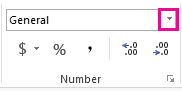
On the Home tab, in the Number group, click the arrow next to the Number Format box, and then click the format that you want.
To select a number format from the list of available formats, click More Number Formats, and then click the format that you want to use in the Category list.
Format a number as text
For numbers that should not be calculated in Excel, such as phone numbers, you can format them as text by applying the Text format to empty cells before typing the numbers.
-
Select an empty cell.
-
On the Home tab, in the Number group, click the arrow next to the Number Format box, and then click Text.
-
Type the numbers that you want in the formatted cell.
Numbers that you entered before you applied the Text format to the cells must be entered again in the formatted cells. To quickly reenter numbers as text, select each cell, press F2, and then press Enter.
Need more help?
You can always ask an expert in the Excel Tech Community or get support in the Answers community.
Need more help?
Want more options?
Explore subscription benefits, browse training courses, learn how to secure your device, and more.
Communities help you ask and answer questions, give feedback, and hear from experts with rich knowledge.
Everyone must start somewhere and getting started with Excel 365 will be made easy with this massive article. Grab your coffee and get ready to learn Excel in a practical way.
If you have every wondered how to use an Excel Spreadsheet and how you can learn to use Excel quickly then you have come to the right place. We are delighted to have you visit and I hope we can add some value while you are learning Excel.
For those of you new to The Excel Club, you should familiarise yourself with our Learn and Earn Activities. Yes, that’s right, you can earn while you learn with us. This article will offer you plenty of opportunities to practice what you will learn so if you want to earn while you learn then you need to be familiar with our program (don’t worry, this won’t cost you a cent)
What is Excel and Why should you learn it?
Excel is a software that allows you to create spreadsheets. Spreadsheets, traditionally used by Accountants, allow you to lay out data in rows and columns. Basic functions of the spreadsheet include keeping lists and records, so they are easily stored and sorted and organized. Excel is often used for carrying out quick and complex calculations, summarizing and reporting. However, once you move beyond the basics of Excel, it is a powerful tool used that can be used for business intelligence and data analysis.
Having basics Excel skills are entry level requirements for many job roles, from Accounting to administration. Everyone uses Excel. Having advanced level excel skills have been proven to propel your career and it gives you an edge when looking for a new job or even that promotion.
Getting Started with Excel – Table of Content
So, what are you going to learn? Well, we are going to answer the basics questions asked when getting started and learning how to use Excel.
How do I open and save an Excel Workbook?
What are the ribbons for in Excel?
How do I use Excels Help Options (and Help on Steroids)?
How do I enter data to an Excel worksheet?
How do I enter formula and do calculations in Excel?
How do I navigate a workbook and select data?
How do I use and edit Excels quick access toolbar?
Whats next?
Before we get started and you make that coffee, why don’t you bookmark this article now in your browser for easy reference! This is a long article with a lot in it (there is no point in skipping stuff when you are new to Excel) and you might not get through it all in the one sitting. Once you have it bookmarked, we will be easy to find 😊
How do I open and save an Excel Workbook?
As there are numerous options for saving workbooks and there are templates available when opening workbooks. Tasks such as Opening, closing, and saving workbooks are done daily and understanding your options is important.
To open a new Excel workbook, select file from the ribbon bar and then select New. A template window will be shown to you. This contains the most popular templates, such as Blank Workbook which you will use most often.

In addition to the most used templates, there is also a search bar that will allow you to search for more templates.
To open a Blank workbook left click on the Blank workbook option found on the templates page. A new instance of Excel will open with a blank workbook.

To Save a workbook, select File from the ribbon bar and then select Save As. Navigate to the folder you wish to save your file. Then enter your file name. The name of a file should be descriptive and saved in a place that you will find it.
Most often you will save your file as an Excel Workbook (.xlsx) however you can select other file types from the dropdown.
To open a workbook you have saved already, select File from the ribbon bar and then select Open. You will be shown the most recent files you have been working on for quick access. Left click on any of these files and they will open.
If your file is not in the recent files, you can navigate to the location and once you find the file, left click and it will open.
To save a file you have been working on previously, select File from the ribbon bar and then select Save. This will save updates to the file and keep the same name and file location.
Learn and Earn Activity 1:
In the comments section below, answer the following question
What recommendations would you make for naming workbooks and why?
What are the ribbons?
Ribbons are the tabs found on the top of your Excel Workbook. They include Home, Insert, Page Layout, Formulas, Data, Review, View, and Help. By clicking on any of the tabs, all the commands and options from that tab can be actioned.
The Ribbons are often shown in a condensed format. When you click on a tab, the ribbon will expand. To hold the ribbon in expanded mode, click on the pin on the very left of the ribbon.
The home ribbon contains commands for
- The clipboard – Cut, Copy, Paste
- Formatting – Font, Alignment, number
- Styles – Conditional Formatting and styles
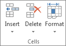
- Cell actions – insert, Delete, Format
- Editing actions – Autosum, Fill, clear, sort/filter and Find & select

The Insert Ribbon contains commands for inserting objects to a worksheet such as
- Tables and Pivot tables
- Pictures and shapes
- Charts
- Sparklines
- Filters, links, and comments
- Text, headers, and footers

The Page Layout ribbon contains commands for
- Setting a theme on the workbook
- Page setup options such as setting margins, print orientations and setting print areas
- Sheet options such as scale to fit and showing/printing gridlines and headings.
- Arrange command for aligning objects in a worksheet

The Formulas Ribbon contains the commands for formulas such as
- Function Library to quickly locate a function you wish to use
- Define Names commands such as Name manager.
- Formula auditing tools and
- Calculation options

The Data Ribbon contains commands for
- Getting and Transforming data
- Filter and Sort commands
- Data tools such as flash fill
- Outline feature such as grouping and ungrouping

The Review ribbon contains commands for
- Proofing such as spell check
- Smart lookups for insights on your data
- Comments and notes
- Worksheet protection

The View ribbon contains commands for
- Workbook views such as page break preview
- Show gridlines, formula bar and headings
- Zoom options
- Window options such as freeze panes

Learn and Earn Activity 2:
In the comments section below answer the following questions
On what ribbon will you find page setup commands?
- Page Layout
- Home
- Insert
- Formulas
On what ribbon will you find the clipboard commands?
- Page Layout
- Home
- Insert
- Formulas
How do I use Excels Help Options (and Help on Steroids)
Both new and experienced Excel users should make themselves familiar with Excels Help feature. No matter what you are doing, F1 will bring up help. When you bring up help you will be met with a predefined list of common help topics.

Clicking on any of the help topics will expand it to a list of articles and videos where you can get further help. These videos can be very useful and are often worth watching as supplementary learning. The search bar can be used to type in what it is that you need help with.
Excel natural language search is like help on steroids. Not only can you get help, but you can also quickly access commands and use smart lookup. To use natural language search just type into the box whatever it is that you are looking for.
If you are working with a business subscription, typing a colleague’s name into the natural language search will bring up the contact details for that colleague. If you type in the name of a file and are using Onedrive or Sharepoint, you can insert them into your current file or open them separately.
Typing in a command, such as Save, will search through excel and if there is a command it will bring up the best match and the arrow keys can be used so select the command you want to perform.

Selecting Help will bring up the help feature that we have already been familiar with.

Selecting Smart Lookup will use Bing, Microsoft search engine, to search the internet for more information and explanations.

In this video, we will take a look at both Help and Excels Natural Language Search so that you are familiar with it before we move on teaching you how to use Excel.
Learn and Earn Activity 3:
In the comments section below tell me which you would prefer to use and why. Excels F1 help feature or Excels natural language search?
How do I enter data?
Data can be entered into Excel in different formats, such as numbers, text and even date and time. You would often see labels in excel, which are most often text which describes the row or column of data.
Before we can enter data, we need to first understand the layout of a worksheet

A cell is any of the boxes you can see on the worksheet. Every cell has an address which is made up of the column letter and row number.
1 – Formula bar. This is used for entering formulas into a cell or range of cells
2 – Cells going across the sheet make up rows. Each row is numbered 1,2…….
3 – cells going down a sheet make up columns. This are lettered A, B, C….
4- An active cell is any cell you click on. Selected cells will be shown with a green box
5 – cell address. This will show the cell address for the active cell. The cell address is the column letter and row number. The active cell is the currently selected cell.
How to enter data into a cell
To enter data into a cell, first, select the cell by clicking on it with the mouse or using the keypad arrows to move to the cell you want. For example, we wish to enter the word Name to Cell A1. First click on cell A1, then using the keyboard enter the text “Name”. To accept the text in the cell press, enter. This will move your active cell down to the next cell below.
We can also enter text data directly into the formulas bar. To do this, again select the cell in which you want the data and then in the formula bar enter the text you want.
To edit the contents of a cell, click or navigate to the cell you wish to edit. Press F2 to turn the cell to edit mode and make any adjustments you need. Once you have made your adjustments, press Enter to accept. You can also edit in the formula bar by selecting the cell and making the edits by selecting the formula bar.
To delete the contents of a cell or cells, select the cells and press delete on your keyboard.
How do I enter a calculation or formula?
The beauty of Excel is its ability to carry out calculations in a fraction of a second. Excel is equipped with many built-in functions from basic arithmetic such as sum and average to more complex engineering and financial functions.
To perform a mathematical operation such as add, subtract, divide or multiply, first select in the cell in which you want to perform the calculation.
All calculations are carried out as a formula. All formulas being with typing = at the start of the cell.
To add two numbers, select the cell and type =1 + 2. When you press enter excel will perform the calculation and return the result. We can do this with any other mathematical operations such as +, -, /, *
You can also carry out calculations on numerical data contains in cells. If we wish to add the contents of multiple cells, we would use the SUM function.
Functions are built-in formulas within excel, such as SUM, AVERAGE, and COUNT.
Functions start with a = and then the functions name followed by a bracket. A screen tip will be displayed showing you tips of what to enter for the function to work.
The SUM function tips look for numbers to add. Click on the cell that contains the first number and you will see this cell reference being entered to the formula. Next, enter a comma, you will see the screen tip jump to the second number, again select the cell. Continue this for each cell you wish to include in your calculation and end with a closing bracket. All formulas end with a closing bracket. Press Enter to accept your formula and the value shown will be the result of the calculation.
Learn and Earn Activity 4
Open a new instance of Excel and carry out the following activities
- In cell A1 type name. In cell B1 type sales
- In cell A2 type Paula. In cell B2 type 20
- In cell A3 type Ava. In cell B3 type 25
- In cell A4 type List. In cell B4 type 22.
- In cell B5 enter a formula that will add all the sales value together.
In the comments section below answer the following questions
- What formula did you use to add all the sales values together?
- What value did you get for the total sales?
How do I navigate a workbook and select data?
We saw when entering data into a cell that pressing enter to accept the contents you entered will move the active cell down one on the worksheet. There are however other navigation options available that will ensure you become more efficient when working with Excel
Below is a table of 16 keyboard shortcuts that will allow you to quickly move around and work with select data. This table is available to download so you have it for handy reference. You should practice these shortcuts as often as possible
| Keys | Action |
| Up Arrow, or Shift+Enter | Move up one cell |
| Down Arrow, or Enter | Down one cell |
| Right Arrow, or Tab | Move right one cell |
| Home | will go to the beginning of the row |
| Ctrl+Home | will go to cell A1 |
| Ctrl+End | Go to the last cell of used range |
| Page Down | Move down one screen (28 rows) |
| Page Up | Move up one screen (28 rows) |
| Ctrl+Right Arrow or Ctrl+Left Arrow | Move to the edge of the current data region |
| Shift+F11 | Insert new sheet |
| Alt+Control+Page Down | Switch to next worksheet |
| Alt+Control+Page Up | Switch to previous worksheet |
| Shift+Arrow keys | Select a range of cells |
| Ctrl+SPACE | Select an entire column |
| Shift+SPACE | Select an entire row |
| Ctrl+Shift+Right Arrow or Ctrl+Shift+Left Arrow | Extend selection to the last nonblank cell in the same column or row as the active cell, or if the next cell is blank, to the next nonblank cell. |
It is important to point out there is a difference between a workbook and a worksheet. A worksheet is the pages in a workbook. You can see the pages as tabs on the bottom of the workbook.
To add a new worksheet to a workbook, click on the + button on the worksheet tabs section.
To rename a worksheet, right click on the tab and select Rename. The cursor will become active in the tab. Once you enter the sheet name, press Enter to accept.
To delete a worksheet, right click on the tab and select delete.

The quick access toolbar allows you to quickly access commands that you use on a regular basis. The toolbar is found on top of the ribbons and it is easy to configure to the commands you use the most
To quickly set up the quick access toolbar customized to suit your needs click on the down arrow to open the Customize quick access toolbar. This will show a list of popular command. By clicking on any of these, you will add them to your quick access toolbar.
For commands that are not included in this list, select More commands
A new box will open with two tables. The table on the left contains the commands available. The table on the right will show what has been added to the quick access toolbar. Select a command from the list on the left by clicking on it, press add, and the quick access toolbar icons should now contain this command. Press ok to accept and the quick access toolbar will update.
To use commands in the quick access toolbar, hover the mouse over the icon and left click.
Learn and Earn Activity 6:
In the comments section below answer the following questions
When writing a formula or mathematical operation such as +,-,*,/ you must start with
- SUM
- The first number to be included in the calculation
- =
“The __________ are identified as tabs which are found on the bottom of a workbook
- Formulas
- Worksheets
- Ribbons
- Quick access tool bar
When you enter data, be it text or numbers, and press enter, the data is accepted into the cell. What happens to the active cell?
- When you press enter the active cell moves down the current column by one row
- When you press enter the active cell moves across the current row by one column
- When you press enter the current cell remain the active cell
What’s next?
Congratulations on reaching the end of this article, you did amazingly well to get this far. Believe it or not, this article makes up the bones of module 1 in our FREE Practical Beginner Excel 365 Course. The next step is to sign up for this free course and continue your learning

In addition to the course, each week we post a new Excel, PowerBI or DAX article with a Learn and Earn Activity. Make sure you are on our email list so you don’t miss out on any of these and you can earn while you learn Excel. You can then use these tokens against the price of our premium training, or you can cash them in or use them against other products and services that now accept STEEM.
Learn and Earn Activity 7
We need your help to get more exposure. Please share this article on your social media profiles, Twitter, Facebook, Instagram, Reddit, where every you can. You can use all or any of the following hashtags #excel #learnexcel #theexcelclub #basicexcel.
In the comments below, share a screenshot or a link to the share and we will reward you with STEEM tokens.
Sign up for my newsletter – Don’t worry, I won’t spam. Just useful Excel and Power BI tips and tricks to your inbox

When you enter any sort of data into Excel, you’ll enter it into a spreadsheet. Of course, starting to enter information is as simple as clicking on a cell in the spreadsheet and typing, but there are some things that are helpful to know – and that you can do – before you ever type that first letter or number.
The first thing you want to do before you type anything is to spend a little time planning the spreadsheet. Beginning to type in Excel is perhaps not as easy as it might be in, let’s say, a word processing program because you’re going to enter all information into rows and columns. A little more organization is required to save you the time of having to create and then recreate the spreadsheet to get it as you want it.
To organize your spreadsheet, you’ll need to determine:
- What is the point of the spreadsheet?
- What information do you need to include?
- What headings are you going to need to explain the information in the spreadsheet?
- Do you want to use columns, rows, or both?
Take a little time to plan out your spreadsheet, and you’ll save yourself a lot of time and headaches down the road.
The Three Types of Data
There are three types of data in Excel: text, value, or formula. This is the type of data you enter into cells. If Excel detects that the entry is a formula, it will calculate the formula and display the result in the cell. You can see the formula in the Formula Bar when the cell is active.
If it detects that it’s not a formula, Excel then decides if it’s text or value. Text entries are aligned to the left side of the cell. Values are aligned to the right.
This is all important to know so you can make sure you are entering things correctly, and Excel is recognizing your entries as the correct data type.
About Text Data
Text entries are simply bits of data that Excel can’t classify as a formula or value. Most text entries are labels. Labels are the names of columns and rows.
You can always tell if Excel is classifying your entry as text because text will be aligned to the left side of the cell.
About Values
Values are the building blocks of all formulas that you enter. Values are numbers that represent quantities, and they are numbers that represent dates.
Values are aligned to the right side of the cell.
If Excel cannot solve the values you add as a formula, it will assume they are values.
Adding Values
Let’s take a look at how to enter values into an Excel worksheet.
Negative values. If you need to add a negative value, enter a minus (-) sign before the value. You can also put in parentheses if you want. Excel will convert it to negative if you choose to use parentheses.
Dollar amounts. If you’re entering a value that’s a dollar amount, you can add dollar signs and commas just like you would if you were writing it by hand.
Decimal points. If you need to add a decimal point, use the period key on your keyboard.
Fractions. If you need to convert a fraction to a decimal, Excel can do that for you, so there’s no need to stress over it yourself. Simply type the fraction in using the slash key on the keyboard. Just make sure you leave a space after any whole numbers before typing in the fraction, as shown below.
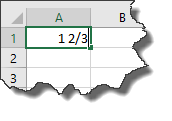
Hit Enter on your keyboard.
As you can see below, Excel classified the number as a value and aligned it to the left. However, it’s still a fraction.
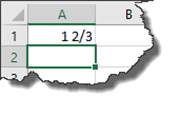
Click on the cell that contains the fraction, then take look at the Formula Bar.
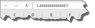
Excel converted it to a decimal.
Note: If you’re entering simple fractions such as 5/8 where a whole number isn’t present, you must enter a zero as the whole number. If you don’t, Excel thinks you’re entering a date.
About Formulas
In Excel, a formula is simply an equation that performs a calculation. It can be as simple as 5 + 2, or as complex as . You can perform calculations within a single cell or based on the values in two different cells, a range of cells, or even a range of cells across several different worksheets. A range of cells is defined as a block or group of cells that have been selected. If all this is confusing right now, don’t worry. It will become crystal clear very soon.
For now, remember that whenever you enter a formula into Excel, the formula must start with an equals sign: =. This might seem strange at first since ordinarily an equals sign comes at the end of an equation, but this lets Excel know right away that you want to perform a calculation. Again, whenever you want to add a formula in Excel, you always start with the equal sign, as shown below:
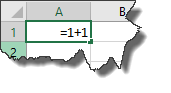
Once you’ve entered it into the cell, either hit Enter or the arrow key to go to another cell.
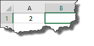
Excel performs the calculation and displays the answer in the cell.
Now whenever you click on the cell, the formula will appear in the Formula Bar.
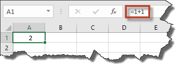
Fixing Decimal Points
If you need to enter a bunch of numbers that use the exact same number of decimal places, you can use Excel’s Fixed Decimal setting so that Excel automatically adds the decimal point for you.
To do this, click the File tab to go to the Backstage area, then click Options.
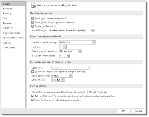
Go to the column on the left, and click Advanced.
Go to Automatically Insert a Decimal Point and put a check in the box.
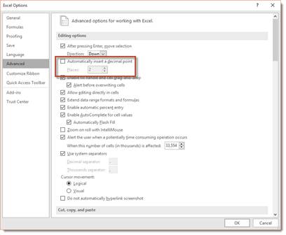
By default, it’s set to two places from the left. You can change this number if needed.
Entering Dates
Dates and times are values in a worksheet, not text. They are values because they can be used for formulations, such as how many days an employee worked last month. In saying that, Excel determines that you’re entering a date or time by the way you type it in.
These are the ways you can type a time into Excel so that it recognizes it as a value:
-
5 AM or 5 PM
-
5 A or 5 P
-
5:46 AM or 5:46 PM
-
5:46:12 AM or 5:46:12 PM
-
17:46
-
17:46:12
Below are the date formats that Excel recognizes as values:
-
May 1, 2016 or May 1, 13. It will appear in Excel as 1-May-13
-
5/1/13 or 5-1-13. It will appear as 5/1/2016
-
1-May-13 or 1/May/13 or 1May13. It will appear as 1-May-2016.
-
May-1 or May/1 or May1 will appear as 1-May.
Note: You only need to enter the last two digits of the year for this century if the last two digits are 00-29. Starting with 2030, you need to enter all four digits.
Entering Data into a Worksheet
Now that we’ve covered some of the very basics of data, it’s time to start actually entering information into Excel. Entering information is as easy as clicking on a cell. When you click on a cell, the cell will be highlighted with a border as shown below.
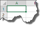
Once it’s highlighted with border, you can type inside of it. When you’re finished entering information into one cell, you can click the mouse in another cell to type more information.
However, moving and clicking your mouse each time you want to change cells becomes time consuming. Most people who use Excel want to move a little faster than that and save as much time as possible. That said, you can also use the following keys to navigate the spreadsheet as you enter information.
-
Enter. Enters the data into the current cell, then moves the cursor to the next cell in the same column. In other words, using the example above, if we pressed ‘Enter’ it would move the cursor down to cell A2. We could then type in A2.
-
Tab. Tab enters the data into the current cell, then moves on cell over in the same row. In this example, it would move to B1.
-
Arrows. You can navigate through columns or rows in the spreadsheet using the arrows.
-
Esc. Cancels the current entry
Entering Labels for Columns and Rows
Labels are used for things such as titles, headings, names, and for identifying columns that contain data. These are text values.
Below we’ve created the beginning of a spreadsheet that will be used to calculate the sales for each employee by the month.
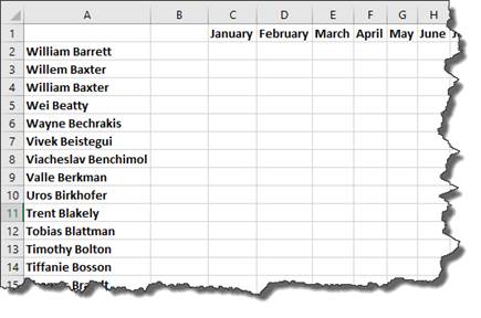
As you can see, Excel recognized our entries as text values. Text values are always aligned to the left side of the cell.
Entering Repeated Labels
Now, let’s say we want to add the first name, William Barrett, twice in our spreadsheet.
A method that you can use to quickly enter repeated labels is to use the Pick List feature. To use the Pick List feature, right click on the cell where you want the label to appear. Select ‘Pick from Drop-down List.’
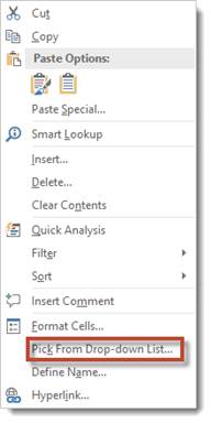
When you click on Pick from Drop-down List, a dropdown menu will appear:
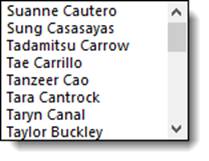
Select the label you want to appear by clicking on it.
For our example, we would scroll down until we found William Barrett, then we’d click on the name. The text label William Barrett is now entered in the cell.
By default, whenever you’re in a cell in Excel and hit the Enter/Return key, the cursor would go down one cell.
In most cases, this is what you want (especially during data entry when you want to move to the next cell below)
But I’ve also come across many scenarios where users do not want to move the cursor to the next cell. They want the cursor to remain on the same cell when they hit the Enter key.
Now there are two broad scenarios where this is required:
- You hit the Enter key and the cursor stays on the same cell
- you want to hit the enter key and want to move to the next line in the same cell so that you can have multiple lines of data in a cell in Excel
In this tutorial, I will show you how to do both of these things, so that when you hit the enter key the cursor remains on the same cell.
Keyboard Shortcut to Keep the Same Cell Active When you Hit the Enter/Return Key
If all you want is to cursor to remain on the same cell when you hit the enter key, the easiest way would be to use the below keyboard shortcut
ALT + ENTER
To use this keyboard shortcut, hold the ALT key and then press the Enter key.
This keyboard shortcut works just like hitting the Enter key, while keeping the cursor in the active cell.
Bonus Shortcut: If you use SHIFT + ENTER, the cursor would move one cell above.
VBA Code to Change Cursor Movement After the Enter Key
While the keyboard shortcut is great, if you want the change the default movement of the cursor when the enter key is hit, you can do that with a very simple one-line VBA code.
Once the VBA code is executed, whenever you hit the Enter key, the cursor would stay on the same cell and would not move anywhere
Make the Change In All Excel Files (the Entire Excel Application)
Below is the VBA macro code to do this:
Application.MoveAfterReturn = FALSE
Below are the steps to use this VBA macro code:
- Open any Excel workbook (or activate any existing open workbook)
- Click the Developer tab (check this if you can’t see the developer tab in the ribbon)
- Click on Visual Basic (this opens the VB editor)

- Click the View option in the menu
- Click on Immediate Window

- Copy the above code and paste it into the ‘Immediate Window’

- Place the cursor at the end of the code line and hit Enter (this executes that line of code)
- Close the VB Editor
The above steps would run this line of code.
Now when you working on a worksheet in Excel, and you hit Enter key, it would keep you in the same cell and not move you to the cell below.
In the above code, we have changed the MoveAfterReturn property and set it to FALSE.
This property is TRUE by default, which means that whenever you hit the Enter key in the Excel application, it moves to the cell below.
By setting this property to FALSE, we had asked Excel, not to move the cursor when we hit Enter.
One very important thing to know here is that this change will be applied to the entire Excel application. so even if you close the current workbook, and open a new or any other existing workbook, this change would remain in place (unless you revert it by setting the MoveAfterReturn property to TRUE)
To revert this change, so that the cursor starts moving to the cell below when you hit the enter key, you need to follow the same steps shown above and use the below VBA code instead:
Application.MoveAfterReturn = TRUE
Make the Change In Specific Excel Files
If you want the cursor to remain on the same cell when you hit enter in only some specific workbooks, and not the entire Excel application, you can do that as well using a simple VBA code.
To do this, you have to ensure that MoveAfterReturn is set to FALSE in only that specific workbook, and it’s TRUE in all the other workbooks.
And there is a very smart way to do this in Excel.
First, let me give you the VBA code that will do this, and then I will explain where to put this code and how to use this.
'This code is developed by Scott from https://SpreadsheetPlanet.com
Private Sub Workbook_Activate()
Application.MoveAfterReturn = False
End Sub

Private Sub Workbook_Deactivate()
Application.MoveAfterReturn = True
End Sub
Below are the steps to place this code in the workbook where you want the cursor to remain on the active cell when you hit the Enter key:
- Open the Excel workbook where you want to apply this
- Click the Developer tab
- Click on Visual Basic (this opens the VB editor)
- In the ‘Project Explorer’ pane, double-click on the ThisWorkbook object (If you don’t see the Project Explorer, click on View and then click on Project Explorer)

- Copy and Paste the above VBA code in the ThisWorkbook code window

- Save the Workbook as a .xlsm (macro-enabled file). The option comes when you save the file (in the Save as Type drop-down in the Save as dialog box)
Once you have added this code in one specific workbook, the MoveAfterReturn property will be set to FALSE only in this specific workbook and would remain TRUE in all the other workbooks.
So when you open/activate this specific workbook and hit the Enter/Return key when working on any cell in the worksheet, the cursor would stay on the same cell.
But for any other workbook, the cursor would move to the cell below.
Let me also quickly explain what happens with this code and how it works.
The Private Sub Workbook_Activate() part of the code is only run when you activate that specific workbook. so as soon as you open or activate that workbook, the MoveAfterReturn property is set to FALSE.
And as soon as you deactivate this workbook (which could be by moving to any other workbook or application), the Private Sub Workbook_Deactivate() part of the code is executed, which sets the MoveAfterReturn property to TRUE.
This way, we are only changing the MoveAfterReturn property in that specific workbook, and we revert it back to its default setting (which is true) as soon as this specific workbook is deactivated.
Entering New Line In The Same Cell
Another common scenario where you may want to remain on the same cell when you hit enter is when you want to have multiple lines in the same cell.
By default, as soon as you hit the Enter key, whatever you have entered in the cell remains and the cursor moves to the next cell.
But what if you want to have multiple lines in the same cell (as shown below).
You can achieve this easily by using the below keyboard shortcut
ALT + ENTER
To use this keyboard shortcut, enter any text that you want to have as the first line in the cell, place the cursor at the end of the line, and then use the above keyboard shortcut by holding the alt key and then pressing the enter key.
ALT + ENTER works as a carriage return where it starts a new line in the same cell.
So these are some of the methods that you can use to stay in the same cell when you hit the Enter or Return key.
If you only need to do this occasionally, you can use the keyboard shortcut CONTROL + ENTER, but in case you need this functionality to be more permanent, you can use the VBA code method.
And finally, if you want to start a new line in the same cell in Excel, you can use the keyboard shortcut ALT + ENTER
I hope you found this Excel tutorial helpful.
Other Excel guides that may also be useful:
- How to Enter Sequential Numbers in Excel? 4 Easy Ways!
- How to Add Bullet Points in Excel (7 Easy Ways)
- How to Unmerge All Cells in Excel? 3 Simple Ways
- Highlight Cell If Value Exists in Another Column in Excel
- How to Remove Panes in Excel Worksheet (Shortcut)
- Edit Cell in Excel (Keyboard Shortcut)