
To find the mean in Excel, you start by typing the syntax =AVERAGE or select AVERAGE from the formula dropdown menu. Then, you select which cells will be included in the calculation. For example: Say you will be calculating the mean for column A, rows two through 20. Your formula will look like this: =AVERAGE(A2:A20).
Contents
- 1 What is mean function in Excel?
- 2 How do you find the mean?
- 3 How do you find the mean median and mode?
- 4 How does mean work?
- 5 How do you solve a mean problem?
- 6 How do you find the mean of the following data?
- 7 What is a mean in a data set?
- 8 How do you calculate mean with examples?
- 9 Is mean the same as average?
- 10 When to use median vs mean?
- 11 How do you find the mean of two means?
- 12 How do you find the mean of grouped data?
- 13 How do I find the mean shortcut method?
- 14 How do you find the sample mean of a data set?
- 15 How do you find the mean of two sets of data?
- 16 How do you find mean in a table?
- 17 How do you calculate mean manually?
- 18 What are the three methods to find mean?
- 19 What does a mean score mean?
- 20 What is the difference between mean and means?
What is mean function in Excel?
The mean or the statistical mean is essentially means average value and can be calculated by adding data points in a setand then dividing the total, by the number of points. Excel’s AVERAGE function does exactly this: sum all the values and divides the total by the count of numbers.
The mean is the same as the average value of a data set and is found using a calculation. Add up all of the numbers and divide by the number of numbers in the data set.
How do you find the mean median and mode?
The arithmetic mean is found by adding the numbers and dividing the sum by the number of numbers in the list. This is what is most often meant by an average. The median is the middle value in a list ordered from smallest to largest. The mode is the most frequently occurring value on the list.
How does mean work?
The mean is the total of the numbers divided by how many numbers there are. To find the mean, add all the numbers together then divide by the number of numbers.
How do you solve a mean problem?
It is easy to calculate: add up all the numbers, then divide by how many numbers there are. In other words it is the sum divided by the count.
How do you find the mean of the following data?
To find the mean of a data set, add all the values together and divide by the number of values in the set. The result is your mean!
What is a mean in a data set?
average
The mean of a set of numbers, sometimes simply called the average , is the sum of the data divided by the total number of data. Example 1 :There are 8 numbers in the set. Add them all, and then divide by 8 .
How do you calculate mean with examples?
For example, take this list of numbers: 10, 10, 20, 40, 70. The mean (informally, the “average“) is found by adding all of the numbers together and dividing by the number of items in the set: 10 + 10 + 20 + 40 + 70 / 5 = 30.
Is mean the same as average?
Average, also called the arithmetic mean, is the sum of all the values divided by the number of values. Whereas, mean is the average in the given data. In statistics, the mean is equal to the total number of observations divided by the number of observations.
When to use median vs mean?
Mean is the most frequently used measure of central tendency and generally considered the best measure of it. However, there are some situations where either median or mode are preferred. Median is the preferred measure of central tendency when: There are a few extreme scores in the distribution of the data.
How do you find the mean of two means?
A combined mean is a mean of two or more separate groups, and is found by : Calculating the mean of each group, Combining the results.
To calculate the combined mean:
- Multiply column 2 and column 3 for each row,
- Add up the results from Step 1,
- Divide the sum from Step 2 by the sum of column 2.
How do you find the mean of grouped data?
To calculate the mean of grouped data, the first step is to determine the midpoint of each interval or class. These midpoints must then be multiplied by the frequencies of the corresponding classes. The sum of the products divided by the total number of values will be the value of the mean.
How do I find the mean shortcut method?
To calculate mean deviation about mean by shortcut method, *First take an appropriate ‘Assumed Mean’ A. *calculate the sum of the frequencies, ∑i=1nfi . *calculate ∑i=1nfidi where, di=xi−A .
How do you find the sample mean of a data set?
The following steps will show you how to calculate the sample mean of a data set: Add up the sample items. Divide sum by the number of samples. The result is the mean.
How do you find the mean of two sets of data?
How to Find the Mean: Overview. To find the arithmetic mean of a data set, all you need to do is add up all the numbers in the data set and then divide the sum by the total number of values.
How do you find mean in a table?
It is easy to calculate the Mean: Add up all the numbers, then divide by how many numbers there are.
How do you calculate mean manually?
The mean, or average, is calculated by adding up the scores and dividing the total by the number of scores.
The mean is calculated in the following manner:
- 3 + 4 + 6 + 6 + 8 + 9 + 11 = 47.
- 47 / 7 = 6.7.
- The mean (average) of the number set is 6.7.
What are the three methods to find mean?
There are three methods for finding the mean from a grouped frequency table.
- Method 1: Direct method.
- Method 2: Assumed Mean method.
- Method 3: Step Deviation method.
What does a mean score mean?
A mean scale score is the average performance of a group of students on an assessment. Specifically, a mean scale score is calculated by adding all individual student scores and dividing by the number of total scores. It can also be referred to as an average.
What is the difference between mean and means?
Mean is the base form and means is the fifth form of verb ‘mean’. In other way,we can also say that mean is plural and means is singular.
There are many functions in order to find the average in Excel (although it does not matter what kind of value it is: numerical, textual, percentage or other). And each of them has its own peculiarities and advantages. After all, certain conditions can be put in this task.
For example, the average in Excel is counting using statistical functions. You can also manually enter your own formula. Consider the various options.
How to find the arithmetic mean?
It is necessary to add all the numbers in the set and divide the sum by the number in order to find the arithmetic mean. For example, the student’s marks in computer science: 3, 4, 3, 5, 5. The average rating is 4 for a quarter. We found the arithmetic mean using the formula: =(3 + 4 + 3 + 5 + 5) / 5.
How can you quickly do this with Excel functions? Take for example a number of random numbers in a row:

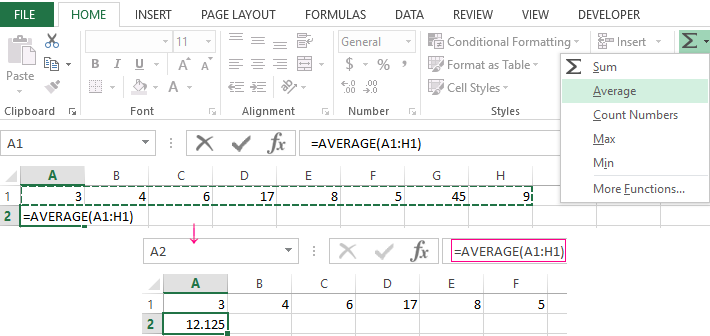
- We put the cursor in cell A2 (under a set of numbers). In the menu – «HOME»-«Editing»-«AutoSum»-«Average» button. A formula appears after clicking in the active cell. Select the range: A1: H1 and press ENTER.
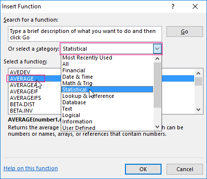
- The second method is based on the same principle of finding the arithmetic mean. But we will call the function AVERAGE differently. Using the function wizard (use fx button or key combination SHIFT + F3).
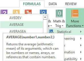
- The third way to call the AVERAGE function from the panel: «FORMULAS»-«More Function»-«Statistical»-«AVERAGE».
Or you can make cell to be active and just manually enter the formula: =AVERAGE(A1:A8).
Now let’s see what the AVERAGE function be able to:
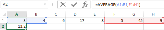
Let us find the arithmetic mean of the first two and three last numbers. Formula: =AVERAGE(A1:B1,F1:H1).
Average value by condition
A numerical criterion or a textual criterion can be the condition for finding the arithmetic mean. We will use the function: = AVERAGEIF().
Find the arithmetic mean for numbers that are greater or equal to 10.
Function:
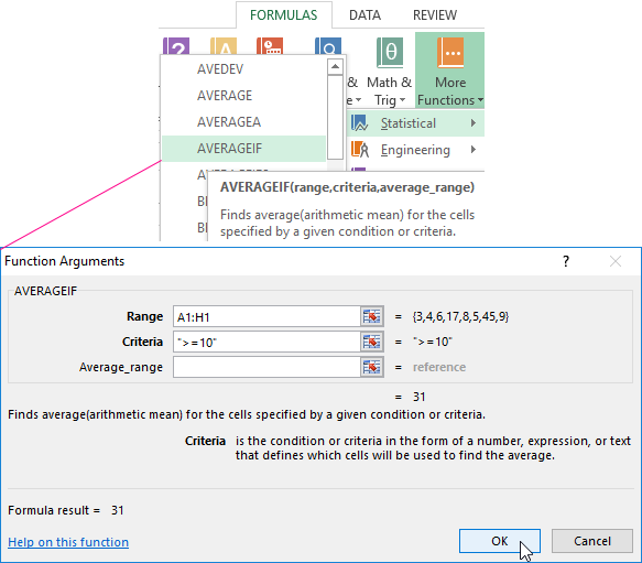
The result of using the function «AVERAGEIF» by the condition «>=10» is next:
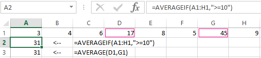
The third argument «Averaging Range» is omitted. Firstly, it is not necessary. Secondly, the range analyzed by the program contains ONLY numeric values. In the cells specified in the first argument, the search will be performed according to the condition specified in the second argument.
Attention! You can specify the search criteria in the cell. And in the formula make a reference to it.
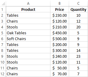
Let’s find the average value of numbers by the text criterion. For example, the average sales of goods «Tables».
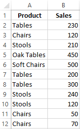
The function will look like this:
Range is a column with the names of goods. Search criteria is a link to a cell with the word «Tables» (you can insert the word «Tables» instead of the A7 link). The averaging range is the cells from which data will be taken to calculate the arithmetic mean.
We get the following value as a result of calculating using the function:
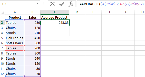
Attention! It is mandatory to point the averaging range for the text criterion (condition).
How to calculate the weighted average price in Excel?
How to calculate the average percentage in Excel? For this purpose, the SUMPRODUCTS and SUM functions are suitable. Table for an example:
How did we know the weighted average price?
Formula:
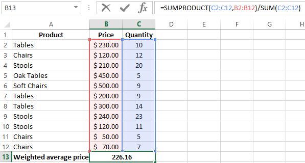
Using the formula =SUMPRODUCT() we learn the total revenue after the realization of the entire quantity of goods. And the =SUM() function sums the goods quantity. We found a weighted average price having divided the total revenue from the sale of goods by the total number of units of the goods. This indicator takes into account the «weight» of each price and its share in the total mass of values.
The standard deviation: the formula in Excel
There is a standard deviation in the entire population and in the sampling. In the first case, this is the square root of the general variance. In the second, this is a square root of the sampling variance.
A dispersion formula is compiled to calculate this statistical indicator. The square root is extracted from it. But in Excel, there is a ready-made function for finding the root-mean-square deviation.
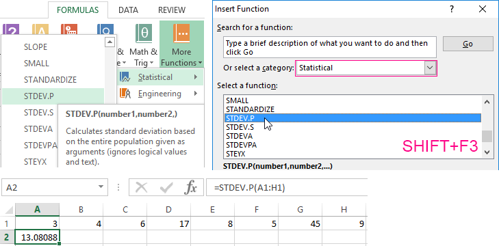
The root-mean-square deviation is related to the scope of the initial data. This is not enough for a figurative representation of the variation of the analyzed range. The coefficient of variation is calculated to obtain the relative level of the data variability.
standard deviation / arithmetic mean
The formula in Excel is as follows:
STDEV.P (range of values) / AVERAGE (range of values).
The coefficient of variation is considered as a percentage. Therefore, set the percentage format in the cell set.
How to Find Mean in Excel (Table of Content)
- Introduction to Mean in Excel
- Example of Mean in Excel
Introduction to Mean in Excel
The average function is used to calculate the Arithmetic Mean of the given input. It is used to do sum of all arguments and divide it by the count of arguments where the half set of the number will be smaller than the mean, and the remaining set will be greater than the mean. It will return the arithmetic mean of the number based on provided input. It is an in-built Statistical function. A user can give 255 input arguments in the function.
As an example, suppose there is 4 number 5,10,15,20 if a user wants to calculate the mean of the numbers then it will return 12.5 as the result of =AVERAGE (5, 10, 15, 20).
The formula of Mean: It is used to return the mean of the provided number where a half set of the number will be smaller than the number, and the remaining set will be greater than the mean.
The argument of the Function:
- number1: It is a mandatory argument in which functions will take to calculate the mean.
- [number2]: It is an optional argument in the function.
Examples on How to Find Mean in Excel
Here are some examples of how to find mean in excel with the steps and the calculation
You can download this How to Find Mean Excel Template here – How to Find Mean Excel Template
Example #1 – How to Calculate the Basic Mean in Excel
Let’s assume there is a user who wants to perform the calculation for all numbers in Excel. Let’s see how we can do this with the average function.
Step 1: Open MS Excel from the start menu >> Go to Sheet1, where the user has kept the data.
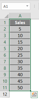
Step 2: Now create headers for Mean where we will calculate the mean of the numbers.
![]()
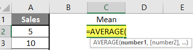
Step 3: Now calculate the mean of the given number by average function>> use the equal sign to calculate >> Write in cell C2 and use average>> “=AVERAGE (“
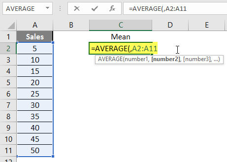
Step 3: Now, it will ask for a number1, which is given in column A >> there are 2 methods to provide input either a user can give one by one or just give the range of data >> select data set from A2 to A11 >> write in cell C2 and use average>> “=AVERAGE (A2: A11) “
Step 4: Now press the enter key >> Mean will be calculated.
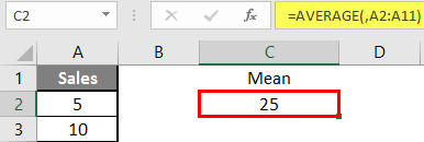
Summary of Example 1: As the user wants to perform the mean calculation for all numbers in MS Excel. Easley everything calculated in the above excel example, and the Mean is 27.5 for sales.
Example #2 – How to Calculate Mean if Text Value Exists in the Data Set
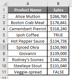
Let’s calculate the Mean if there is some text value in the Excel data set. Let’s assume a user wants to perform the calculation for some sales data set in Excel. But there is some text value also there. So, he wants to use count for all, either its text or number. Let’s see how we can do this with the AVERAGE function. Because in the normal AVERAGE function, it will exclude the text value count.
Step 1: Open MS Excel from the start menu >> Go to Sheet2, where the user has kept the data.
Step 2: Now create headers for Mean where we will calculate the mean of the numbers.
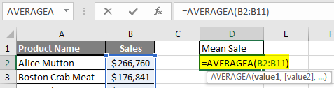
Step 3: Now calculate the mean of the given number by average function>> use the equal sign to calculate >> Write in cell D2 and use AVERAGEA>> “=AVERAGEA (“
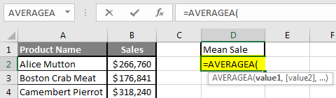
Step 4: Now, it will ask for a number1, which is given in column B >> there is two open to provide input either a user can give one by one or just give the range of data >> select data set from B2 to B11 >> write in D2 Cell and use average>> “=AVERAGEA (D2: D11) “
Step 5: Now click on the enter button >> Mean will be calculated.
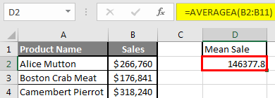
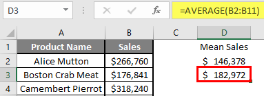
Step 6: Just to compare the AVERAGEA and AVERAGE, in normal average, it will exclude the count for text value so mean will high than the AVERAGE MEAN.
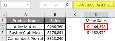
Summary of Example 2: As the user wants to perform the mean calculation for all number in MS Excel. Easley, everything calculated in the above excel example and the Mean is $146377.80 for sales.
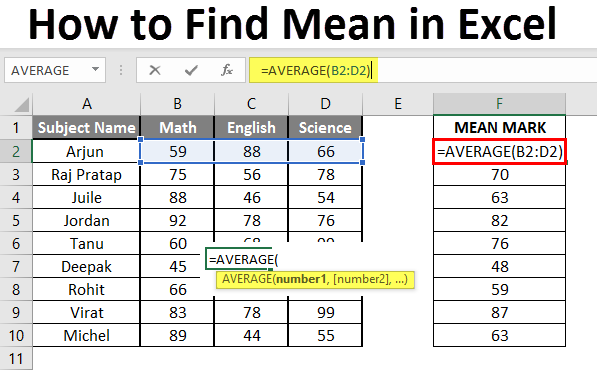
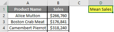
Example #3 – How to Calculate Mean for Different Set of Data
Let’s assume a user wants to perform the calculation for some student’s mark data set in MS Excel. There are ten student marks for Math, English, and Science out of 100. Let’s see How to Find Mean in Excel with the AVERAGE function.
Step 1: Open the MS Excel from the start menu >> Go to Sheet3, where the user kept the data.
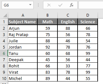
Step 2: Now create headers for Mean where we will calculate the mean of the numbers.
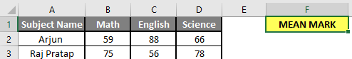
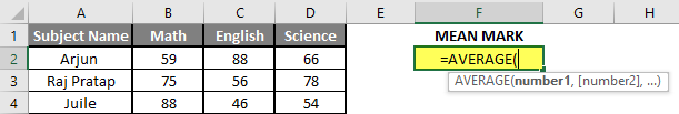
Step 3: Now calculate the mean of the given number by average function>> use the equal sign to calculate >> Write in F2 Cell and use AVERAGE >> “=AVERAGE (“
Step 3: Now, it will ask for number1 which is given in B, C, and D column >> there is two open to provide input either a user can give one by one or just give the range of data >> Select data set from B2 to D2 >> Write in F2 Cell and use average >> “=AVERAGE (B2: D2) “
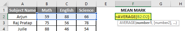
Step 4: Now click on the enter button >> Mean will be calculated.
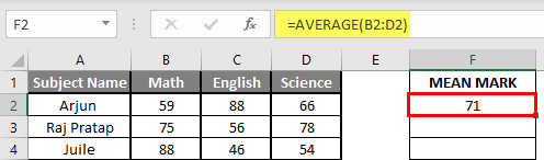
Step 5: Now click on the F2 cell and drag and apply to another cell in the F column.
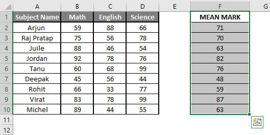
Summary of Example 3: As the user wants to perform the mean calculation for all number in MS Excel. Easley, everything calculated in the above excel example and the Mean is available in the F column.
Things to Remember About How to Find Mean in Excel
- Microsoft Excel’s AVERAGE function used to calculate the Arithmetic Mean of the given input. A user can give 255 input arguments in the function.
- Half the set of a number will be smaller than the mean, and the remaining set will be greater than the mean.
- If a user calculating the normal average, it will exclude the count for a text value, so AVERAGE Mean will bigger than the AVERAGE MEAN.
- Arguments can be number, name, range or cell references that should contain a number.
- If a user wants to calculate the mean with some condition, then use AVERAGEIF or AVERAGEIFS.
Recommended Articles
This is a guide to How to Find Mean in Excel. Here we discuss How to Find Mean along with examples and a downloadable excel template. You may also look at the following articles to learn more –
- FIND Function in Excel
- Excel Find
- Excel Average Formula
- Excel AVERAGE Function
This tutorial will explain and elaborate on how to calculate Mean in Excel along with easy steps and examples. Indeed Microsoft excel is designed to analyze and organize numerical data quickly.
For this reason measure of central tendency is a big part thus basically used to represent and identify the central position within the data provided or, more technically, the middle or center in a statistical distribution. Sometimes, they are also classified as summary statistics.
The three main measures of central tendency are Mean, Median and Mode. They all are valid measures of a central location, but each gives a different indication of a typical value, and under different circumstances, some measures are more appropriate to use than others.
Particularly, we will be focused on how to get the MEAN of supplied data
Mean formula in Excel
The mean function is one of the three main measure of central tendency. It is basically known as average of cells was calculated by adding up all the collection of data sets and dividing it by the number of counts.
These mathematical terms including median and mode have different ways of examining the set of data or numbers. Consequently, Excel provides built-in function determining these terms except range, which requires formula to obtain the output.
Furthermore, MEAN is one of the crucial functions in terms of analyzing data. Therefore it is not a waste when you know how to use it. It is helpful considering instances of finalizing the students’ grades or even product sales.
One more thing that MEAN or average function can do is to ignore cells omitting numbers and empty cells. But if you want to include empty cells or values specified as zero, you can use AVERAGEA function which is more likely the same.
The good thing about finding MEAN is that the function you’re gonna use is still available on the following; excel for Microsoft 365, excel 2010, excel 2016, excel 2019, and excel 2021.
Syntax of Mean
=Average(value1,[value2]...)
Return Value
Average of the set of numerical values
Arguments
value1: required its the values needed to calculate MEAN.value2:Optional.Values to calculate.
There are bunches of ways to calculate the MEAN of your data in your spreadsheet, it will depend on what data you are trying to exercise. So here are the simple steps to find your mean.
- Create the data you will use in your workbook.
Open your Microsoft Excel, and analyze what data you need. You can have any data such as order sales, student grades, employee salaries, or whatever suits your perspective. Make use of the columns and rows as it is favorable when doing hands-on take advantage to create your design and creativity.
- Reorganize your Excel spreadsheet as needed
If you imported data in your workbook reorganize those data and format it according to the requirements. Actually, this step is not required to finish since you are at hand making your data; it is up to you how you would like to rearrange the data.
- Select an empty cell to enter the mean formula
Calculating MEAN in your excel spreadsheet could be done on the same worksheet you’re analyzing. Select an empty cell so you will not lose any data in the worksheet. You can prefer to be at the bottom of the column or at the right side depending on what is easy for you.
- Press Enter to the formula to find the mean
After you created a formula, just hit enter key to completely see the Mean of your data.
As we have probably known the arithmetic mean is also understood as average. Thus let’s see how to calculate the average, will give few example formulas and instances to clearly understand it.
Basically, to get the mean of a group of numbers: {2,4,6,7, 8,10,12}.
Add them up and then divide the sum by the total number of set: {2,4,6,7, 8,10,12}/7=6
Take a look at this another sample:
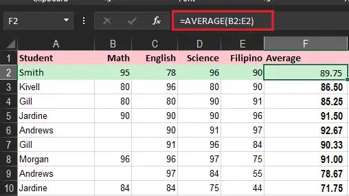
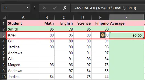
Supposedly you are going to get the mean of Smith’s subjects’ scores.
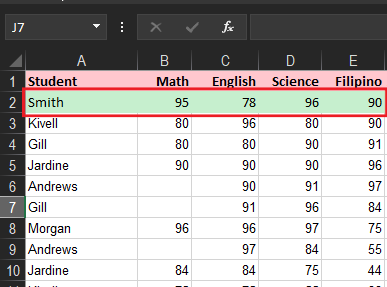
- To get the Mean use this formula: =AVERAGE(B2:E2)
To get the average of only “Kivell” grades, use an AVERAGEIF formula:
=AVERAGEIF(A2:A10,"Kivell",C3:E3)
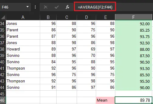
To calculate the mean of all the student’s averages
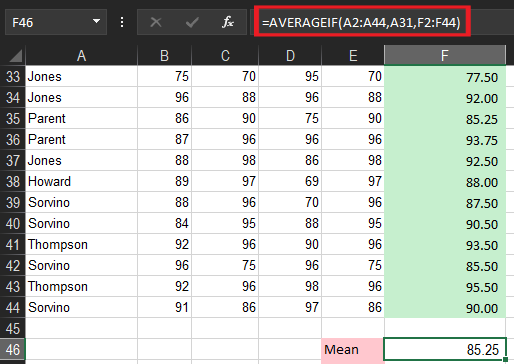
You can also enter your conditions in separate cells, and reference those cells in your formulas, like this:
=AVERAGEIF(A2:A44,A31,F2:F44)
Reminders for Specifying MEAN calculation criteria
There are more often that you need to meet certain criteria in order to obtain the mean of data. Here are circumstances you will use more specific mean formulas to acquire specified information needed in the calculation.
- AVERAGEA: If you need to include text or zero value in your calculations.
- AVERAGEIF: Utilize this formula if you want to get the mean which needs to meet a single criterion of certain information. For instance, you need to find the cells that do not meet a quota or the passing average.
- AVERAGE IF: Finding MEAN which meets multiple criteria. This scenario implies two or more requirements need to find the MEAN of a sample data, thus use this formula to find the mean of a certain range.
What does ref mean on excel?
The #REF error you encountered when applying your formula is because the formula refers to a cell that is not valid. It always occurs when your cells used as references are pasted or deleted.
Summary
Recap on this tutorial How To Calculate Mean on Excel there are several ways to calculate MEAN from single criteria to two or more, including text values. Finding MEAN is similar to average and it uses the same function. Besides, it is beneficial in analyzing data in business, study, and daily activities.
There we have already done what MEAN is. For further clarification and suggestions feel free to leave your comment!
Thank you for reading!
Calculating the mean of numbers is one of staples of statistical analysis processes. In this article, we’re going to show you how to calculate mean in Excel using the AVERAGE formula.
Syntax
=AVERAGE( array of numbers )
Steps
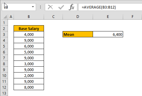
- Begin by creating the formula =AVERAGE(
- Select your data range that contains the values (i.e. B3:B12)
- Finish the formula with ) and press the Enter key.
How to find the mean in Excel
The mean or the statistical mean is essentially means average value and can be calculated by adding data points in a setand then dividing the total, by the number of points. Excel’s AVERAGE function does exactly this: sum all the values and divides the total by the count of numbers.
The AVERAGE function can also be configured to ignore empty cells and cells that do not include any numbers. If you want to include empty or invalid values in calculations as zeroes, use the AVERAGEA function. The AVERAGEA function works exactly the same with the AVERAGE.
=AVERAGEA( array of numbers )
For more information about AVERAGE formula please see our related article.
In this guide, I will show you how to calculate the mean (average), standard deviation (SD) and standard error of the mean (SEM) by using Microsoft Excel.
Calculating the mean and standard deviation in Excel is pretty easy. These have built-in functions already available.
Calculating the standard error in Excel, however, is a bit trickier. There is no formula within Excel to use for this, so I will show you how to calculate this manually.
How to calculate the mean value in Excel
The mean, or average, is the sum of the values, divided by the number of values in the group.
To calculate the mean, follow the steps below.
1. Click on an empty cell where you want the mean value to be.
2. Enter the following formula.
=AVERAGE(number1:number2)
Then change the following:
- Number1 – the cell that is at the start of the list of values
- Number2 – the cell that is at the end of the list of values
You can simply click and drag on the values within Excel instead of typing the cell names.
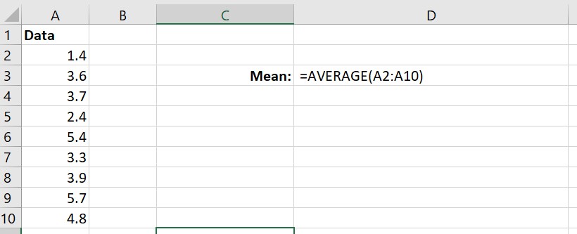
3. Then press the ‘enter’ button to calculate the mean value.
How to calculate the standard deviation in Excel
The standard deviation (SD) is a value to indicate the spread of values around the mean value.
To calculate the SD in Excel, follow the steps below.
1 Click on an empty cell where you want the SD to be.
2. Enter the following formula
=STDEV(number1:number2)
Then, as with the mean calculation, change the following:
- Number1 – the cell that is at the start of the list of values
- Number2 – the cell that is at the end of the list of values
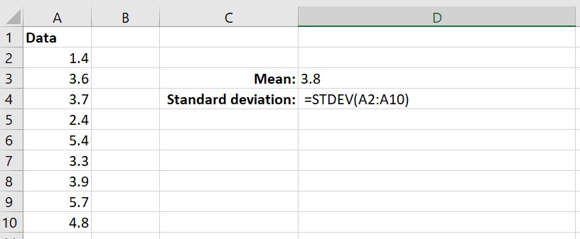
3. Then press the ‘enter’ button to calculate the SD.
How to calculate the standard error in Excel
The standard error (SE), or standard error of the mean (SEM), is a value that corresponds to the standard deviation of a sampling distribution, relative to the mean value.
The formula for the SE is the SD divided by the square root of the number of values n the data set (n).
To calculate the SE in Excel, follow the steps below.
1. Click on an empty cell where you want the SE to be.
2. Enter the following into the cell:
=STDEV(number1:number2)/SQRT(COUNT(number1:number2))
Change the following throughout:
- Number1 – the cell that is at the start of the list of values
- Number2 – the cell that is at the end of the list of values
It is worth noting that instead of using the COUNT function, you can simply type in the number of values in the data set. In this example, this would be 9.
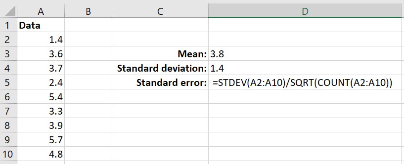
3. Then press the ‘enter’ button to calculate the SE.
Conclusion
In this tutorial, I have described how to calculate the mean, SD and SE by using Microsoft Excel.
Microsoft Excel version used: Office 365 ProPlus
Statistics made easy: Microsoft Excel offers you a function for the automatic calculation of the arithmetic mean – also called “mean” or “average“. To calculate the mean on Excel, the number of values add and then divide all values. In Excel, you can either enter individual values or select cells. In this article, I want to show you a couple of really practical methods on how to find mean on excel and how it works.
In this guide, you will learn the following
How Microsoft Excel Calculates mean on Excel.
The average is basically a value calculated within a set of numbers, which, in mathematics, is known as the arithmetic mean or mean. To calculate it, what we do is add the values and divide them by the total number of numbers.
For example: let’s assume that we have the grades of any subject, in which we have got the following results (3, 4, 5, 3, 5) and we want to calculate the average obtained in that subject. Therefore, to get our average we would do it as follows, first- we add the values (3 + 4 + 5 + 3 + 5) and divide by the number of numbers (5).
The average of the marks obtained will be (3 + 4 + 5 + 3 + 5) / 5 = 4
This method is undoubtedly good, but the convenience of its use is significantly limited by the volume of processed data because it will take a lot of time to enumerate all the numbers or coordinates of cells in a large array, in this case, we can follow the procedure below to find the average on Excel.
Now, to calculate the average on Excel, we don’t have to perform all that operation, we just have to call the AVERAGE function.
To apply the average function in Excel, select an empty cell to enter the mean formula and start the formula with an equal (=), then we write AVERAGE and select the range of which we want to calculate the mean.
= AVERAGE (B2: F2)

Find mean on Excel from Ribbon Tools
This method is based on the use of a special tool on the program tape.
1 Select the range of cells with numeric data for which we want to determine the average value.

2 Go to the “Home” tab. Find the AutoSum icon in the Editing Tools section and click on the small down arrow next to it. In the list that opens, click on the “Average” option.

3 Immediately below the selected range, the result will be displayed, which is the average value for all the selected cells.
4 If we go to the cell with the result, then in the formula bar we will see which function was used for calculations – this is the AVERAGE operator, the arguments of which is the range of cells we have selected.
An alternative way to find mean (average) on Excel.
Go to the first free cell after the column or row (depending on the data structure) and press the keyboard shortcut “Alt+MUA” for calculating the average.
Using the AVERAGE function
1 We stand in the cell where we want to display the result. Click on the “Insert Function” (fx) icon to the left of the formula bar.
2 In the opened window of the Function Wizard, select the “Statistical” category, in the proposed list, click on the “AVERAGE“, and then click OK.

3 A window with function arguments will be displayed on the screen (their maximum number is 255). Mark the coordinates of the required range as the value of the “Number1” argument. This can be done manually by typing the addresses of the cells from the keyboard.
Alternatively, you can first click inside the field to enter information and then use the left mouse button to select the required range on the sheet. If necessary (if you need to mark cells and ranges of cells elsewhere in the sheet), proceed to fill in the “Number2” argument, and so on. When ready, click OK.

4 We get the result in the selected cell.
Tools in the Formulas tab
Excel has a special tab responsible for working with formulas. In the case of calculating the average, it can also come in handy.
1 We select the cell in which we want to perform calculations. Go to the “Formulas” tab. In the “Functions Library” section of the tools, click on the “More Functions” icon, in the list that opens, select the “Statistical” group, then – “AVERAGE“.

2 The already familiar window of arguments for the selected function will open. Fill in the data and click the OK button.
Calculate average with a condition (AVERAGEIF)
Through the Excel spreadsheet, we can also calculate the average according to a given condition or criterion. We can do this through the AVERAGE function.
The AVERAGEIF function helps us find the average (arithmetic mean) of the cells that meet a certain condition.
AVERAGEIF function syntax
AVERAGEIF (range, criterion, [average_range])
- Range: It is the range of cells where the criteria will be searched.
- Criterion: It is the condition or criteria as a number, expression, or text that determines which cells will find the average.
- Average_range: These are the cells that will find the average. If omitted, the cells in the range will calculate the average.
Example: We need to get the average sale price of the HP laptop product in the technology category.
To calculate the average sale price of the portable product we are going to use the AVERAGEIF function and we are going to start our formula with the equal sign (=), then we are going to choose the range where our criterion is, which for our example is in B2: B20 and the criterion or condition of our formula, located in quotation marks is “HP laptop“. Finally, we choose the range of values where the average will be applied if it meets the criteria that we have established.
= AVERAGEIF (B2: B20, “HP laptop”, E2: E20)

Calculate the average of numbers in non-contiguous cells
In this example, We need to get the average sale price of Sales 1 and Sales 2 in the fashion category.
=AVERAGE(C2:D2,C5:D5,C9:D9)
- So select the cell that will display the result.
- Insert Average function and select cell range C2:D2 and type comma.
- Then select the other cells range C5:D5, C9:D9.
- Close the parenthesis and validate.

![]()
Finding the mean comes in handy when processing and analyzing all kinds of data. With Microsoft Excel’s AVERAGE function, you can quickly and easily find the mean for your values. We’ll show you how to use the function in your spreadsheets.
How Microsoft Excel Calculates the Mean
By definition, the mean for a data set is the sum of all the values in the set divided by the count of those values.
For example, if your data set contains 1, 2, 3, 4, and 5, the mean for this data set is 3. You can find it with the following formula.
(1+2+3+4+5)/5
You could type out formulas like that yourself, but Excel’s AVERAGE function helps you perform this calculation with ease.
Find the Mean Using a Function in Microsoft Excel
In our example, we’ll find the mean for the values in the “Score” column, and display the answer in the C9 cell.
We’ll start by clicking the C9 cell where we want to display the resulting mean.

In the C9 cell, we’ll type the following function. This function finds the mean for the values in all the cells between C2 and C6 (both these cells included).
=AVERAGE(C2:C6)
Press Enter and the result will appear in the C9 cell.
You can use the AVERAGE function to find the mean for any values in your spreadsheet. Enjoy!
Getting the mean will come in handy if you ever need Excel to calculate uncertainty.
RELATED: How to Get Microsoft Excel to Calculate Uncertainty
READ NEXT
- › How to Calculate Average in Microsoft Excel
- › How to Combine Data From Spreadsheets in Microsoft Excel
- › How to Manage Conditional Formatting Rules in Microsoft Excel
- › How to Calculate the Median in Microsoft Excel
- › HoloLens Now Has Windows 11 and Incredible 3D Ink Features
- › The New NVIDIA GeForce RTX 4070 Is Like an RTX 3080 for $599
- › How to Adjust and Change Discord Fonts
- › This New Google TV Streaming Device Costs Just $20
How-To Geek is where you turn when you want experts to explain technology. Since we launched in 2006, our articles have been read billions of times. Want to know more?
Contents
- 1 How do you calculate mean in Excel 2016?
- 2 What is the mean function in Excel?
- 3 How do you do mean median mode in Excel?
- 4 How do I calculate mean?
- 5 How do you find the median of grouped data in Excel?
- 6 What is the formula of grouped data?
- 7 What is the median of grouped data?
- 8 What is the formula of mode for grouped data?
- 9 Is there a formula for mode?
- 10 What is mode formula?
- 11 How do you solve for mode?
- 12 How do you solve a mode question?
- 13 How do you do range?
- 14 What happens when you have 2 modes?
- 15 Can you have 3 modes?
- 16 What is the mode if there are no repeating numbers?
- 17 What to put if there is no mode?
- 18 What does a mode of 0 mean?
- 19 How do you find the mode when there are two?
- 20 What do you do when there are two medians?
How do you calculate mean in Excel 2016?
Calculate the average of numbers in a contiguous row or column
- Click a cell below, or to the right, of the numbers for which you want to find the average.
- On the Home tab, in the Editing group, click the arrow next to AutoSum , click Average, and then press Enter.
What is the mean function in Excel?
Description. Returns the average (arithmetic mean) of the arguments. For example, if the range A1:A20 contains numbers, the formula =AVERAGE(A1:A20) returns the average of those numbers.
How do you do mean median mode in Excel?
How do I calculate mean?
The mean is the average of the numbers. It is easy to calculate: add up all the numbers, then divide by how many numbers there are. In other words it is the sum divided by the count.
How do you find the median of grouped data in Excel?
What is the formula of grouped data?
To calculate the mean of grouped data, the first step is to determine the midpoint (also called a class mark) of each interval, or class. These midpoints must then be multiplied by the frequencies of the corresponding classes. The sum of the products divided by the total number of values will be the value of the mean.
What is the median of grouped data?
To find the median of a grouped data, we have the formula. Median=l+N2−Ff×h. where l = lower limit of the median class. f = frequency of the median class. F = cumulative frequency of the class preceding the median class.
What is the formula of mode for grouped data?
Mode for grouped data is given as Mode=l+(f1−f02f1−f0−f2)×h , where l is the lower limit of modal class, h is the size of class interval, f1 is the frequency of the modal class, f0 is the frequency of the class preceding the modal class, and f2 is the frequency of the class succeeding the modal class.
Is there a formula for mode?
In this article, we will try and understand the mode function, examples and explanations of each example along with the formula and the calculations. Where, L = Lower limit Mode of modal class. fm = Frequency of modal class.
Mode Formula Calculator.
| Mode Formula = | L + (fm – f1) x h / (fm – f1) + (fm – f2) |
|---|---|
| = | 0 + (0 – 0) x 0 / (0 – 0) + (0 – 0)= 0 |
What is mode formula?
The formula used to find the mode of a grouped or non-grouped data is called mode formula and the value of the observation having the maximum frequency is called mode. Mode = l +(frac{f_{1}-f_{0}}{2f_{1}-f_{0}-f_{2}}times h) Where, l = lower limit of the modal class. h = size of the class interval.
How do you solve for mode?
The mode of a data set is the number that occurs most frequently in the set. To easily find the mode, put the numbers in order from least to greatest and count how many times each number occurs. The number that occurs the most is the mode!
How do you solve a mode question?
How do you do range?
The range is the difference between the smallest and highest numbers in a list or set. To find the range, first put all the numbers in order. Then subtract (take away) the lowest number from the highest. The answer gives you the range of the list.
What happens when you have 2 modes?
A set of numbers can have more than one mode (this is known as bimodal if there are two modes) if there are multiple numbers that occur with equal frequency, and more times than the others in the set.
Can you have 3 modes?
In a set of data, the mode is the most frequently observed data value. There may be no mode if no value appears more than any other. There may also be two modes (bimodal), three modes (trimodal), or four or more modes (multimodal).
What is the mode if there are no repeating numbers?
The “mode” is the value that occurs most often. If no number in the list is repeated, then there is no mode for the list.
What to put if there is no mode?
Thus, If data has no mode then we can’t use mode as a measure of central tendency instead we can use mean, median, etc.
What does a mode of 0 mean?
Answer: The mode of these temperatures is 0. In Example 3, each value occurs only once, so there is no mode. In Example 4, the mode is 0, since 0 occurs most often in the set. Do not confuse a mode of 0 with no mode.
How do you find the mode when there are two?
The mode of a data set is the number that occurs most frequently in the set. To easily find the mode, put the numbers in order from least to greatest and count how many times each number occurs. The number that occurs the most is the mode!