
A PivotTable is a powerful tool to calculate, summarize, and analyze data that lets you see comparisons, patterns, and trends in your data. PivotTables work a little bit differently depending on what platform you are using to run Excel.


-
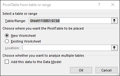
Select the cells you want to create a PivotTable from.
Note: Your data should be organized in columns with a single header row. See the Data format tips and tricks section for more details.
-
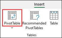
Select Insert > PivotTable.

-
This will create a PivotTable based on an existing table or range.
Note: Selecting Add this data to the Data Model will add the table or range being used for this PivotTable into the workbook’s Data Model. Learn more.
-
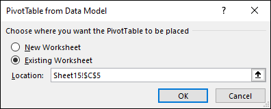
Choose where you want the PivotTable report to be placed. Select New Worksheet to place the PivotTable in a new worksheet or Existing Worksheet and select where you want the new PivotTable to appear.
-
Click OK.
By clicking the down arrow on the button, you can select from other possible sources for your PivotTable. In addition to using an existing table or range, there are three other sources you can select from to populate your PivotTable.
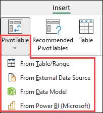
Note: Depending on your organization’s IT settings you might see your organization’s name included in the button. For example, «From Power BI (Microsoft)»
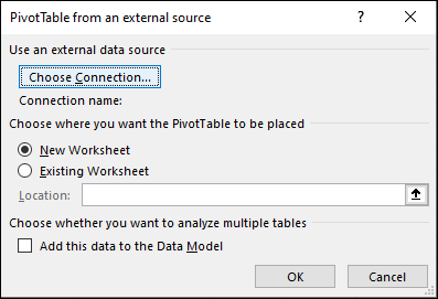
Get from External Data Source
Get from Data Model
Use this option if your workbook contains a Data Model, and you want to create a PivotTable from multiple Tables, enhance the PivotTable with custom measures, or are working with very large datasets.
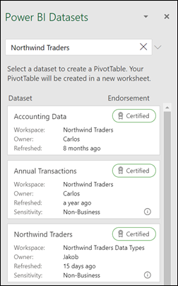
Get from Power BI
Use this option if your organization uses Power BI and you want to discover and connect to endorsed cloud datasets you have access to.
-
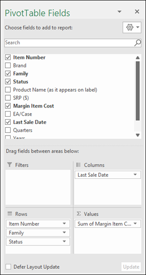
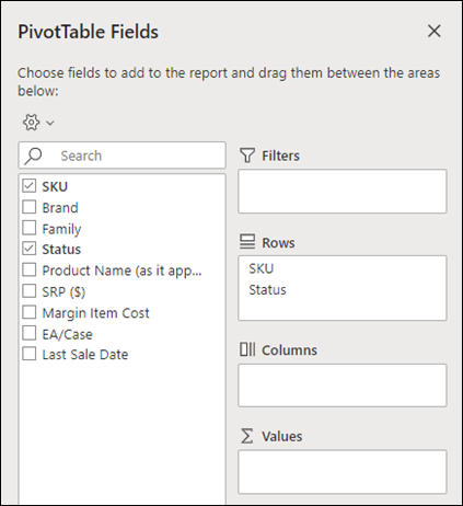
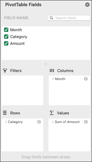
To add a field to your PivotTable, select the field name checkbox in the PivotTables Fields pane.
Note: Selected fields are added to their default areas: non-numeric fields are added to Rows, date and time hierarchies are added to Columns, and numeric fields are added to Values.
-
To move a field from one area to another, drag the field to the target area.
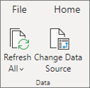
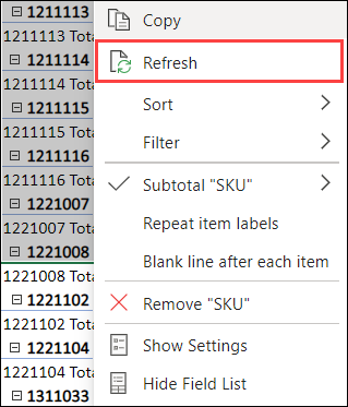
If you add new data to your PivotTable data source, any PivotTables that were built on that data source need to be refreshed. To refresh just one PivotTable you can right-click anywhere in the PivotTable range, then select Refresh. If you have multiple PivotTables, first select any cell in any PivotTable, then on the Ribbon go to PivotTable Analyze > click the arrow under the Refresh button and select Refresh All.
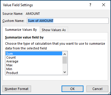
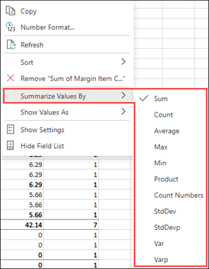
Summarize Values By
By default, PivotTable fields that are placed in the Values area will be displayed as a SUM. If Excel interprets your data as text, it will be displayed as a COUNT. This is why it’s so important to make sure you don’t mix data types for value fields. You can change the default calculation by first clicking on the arrow to the right of the field name, then select the Value Field Settings option.
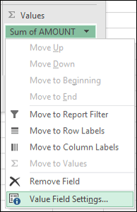
Next, change the calculation in the Summarize Values By section. Note that when you change the calculation method, Excel will automatically append it in the Custom Name section, like «Sum of FieldName», but you can change it. If you click the Number Format button, you can change the number format for the entire field.
Tip: Since the changing the calculation in the Summarize Values By section will change the PivotTable field name, it’s best not to rename your PivotTable fields until you’re done setting up your PivotTable. One trick is to use Find & Replace (Ctrl+H) >Find what > «Sum of«, then Replace with > leave blank to replace everything at once instead of manually retyping.
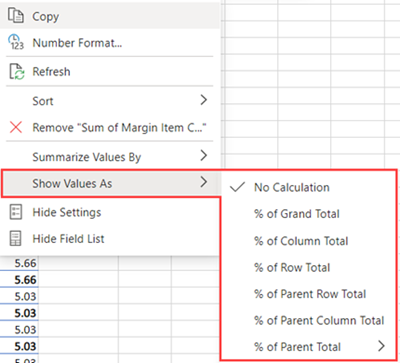
Show Values As
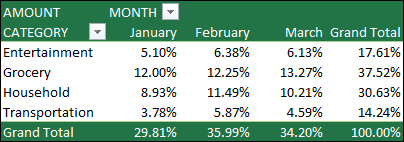
Instead of using a calculation to summarize the data, you can also display it as a percentage of a field. In the following example, we changed our household expense amounts to display as a % of Grand Total instead of the sum of the values.
Once you’ve opened the Value Field Setting dialog, you can make your selections from the Show Values As tab.
Display a value as both a calculation and percentage.
Simply drag the item into the Values section twice, then set the Summarize Values By and Show Values As options for each one.
-
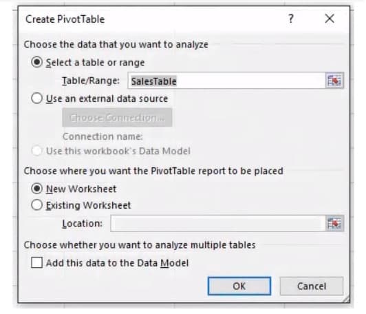
Select a table or range of data in your sheet and select Insert > PivotTable to open the Insert PivotTable pane.
-
You can either manually create your own PivotTable or choose a recommended PivotTable to be created for you. Do one of the following:
-
On the Create your own PivotTable card, select either New sheet or Existing sheet to choose the destination of the PivotTable.
-
On a recommended PivotTable, select either New sheet or Existing sheet to choose the destination of the PivotTable.
Note: Recommended PivotTables are only available to Microsoft 365 subscribers.
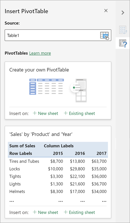
You can change the data sourcefor the PivotTable data as you are creating it.
-
In the Insert PivotTable pane, select the text box under Source. While changing the Source, cards in the pane won’t be available.
-
Make a selection of data on the grid or enter a range in the text box.
-
Press Enter on your keyboard or the button to confirm your selection. The pane will update with new recommended PivotTables based on the new source of data.

Get from Power BI
Use this option if your organization uses Power BI and you want to discover and connect to endorsed cloud datasets you have access to.
In the PivotTable Fields pane, select the check box for any field you want to add to your PivotTable.
By default, non-numeric fields are added to the Rows area, date and time fields are added to the Columns area, and numeric fields are added to the Values area.
You can also manually drag-and-drop any available item into any of the PivotTable fields, or if you no longer want an item in your PivotTable, drag it out from the list or uncheck it.
Summarize Values By
By default, PivotTable fields in the Values area will be displayed as a SUM. If Excel interprets your data as text, it will be displayed as a COUNT. This is why it’s so important to make sure you don’t mix data types for value fields.
Change the default calculation by right clicking on any value in the row and selecting the Summarize Values By option.
Show Values As
Instead of using a calculation to summarize the data, you can also display it as a percentage of a field. In the following example, we changed our household expense amounts to display as a % of Grand Total instead of the sum of the values.
Right click on any value in the column you’d like to show the value for. Select Show Values As in the menu. A list of available values will display.
Make your selection from the list.
To show as a % of Parent Total, hover over that item in the list and select the parent field you want to use as the basis of the calculation.
If you add new data to your PivotTable data source, any PivotTables built on that data source will need to be refreshed. Right-click anywhere in the PivotTable range, then select Refresh.
If you created a PivotTable and decide you no longer want it, select the entire PivotTable range and press Delete. It won’t have any effect on other data or PivotTables or charts around it. If your PivotTable is on a separate sheet which has no other data you want to keep, deleting the sheet is a fast way to remove the PivotTable.
-
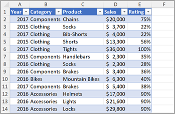
Your data should be organized in a tabular format, and not have any blank rows or columns. Ideally, you can use an Excel table like in our example above.
-
Tables are a great PivotTable data source, because rows added to a table are automatically included in the PivotTable when you refresh the data, and any new columns will be included in the PivotTable Fields List. Otherwise, you need to either Change the source data for a PivotTable, or use a dynamic named range formula.
-
Data types in columns should be the same. For example, you shouldn’t mix dates and text in the same column.
-
PivotTables work on a snapshot of your data, called the cache, so your actual data doesn’t get altered in any way.
If you have limited experience with PivotTables, or are not sure how to get started, a Recommended PivotTable is a good choice. When you use this feature, Excel determines a meaningful layout by matching the data with the most suitable areas in the PivotTable. This helps give you a starting point for additional experimentation. After a recommended PivotTable is created, you can explore different orientations and rearrange fields to achieve your specific results. You can also download our interactive Make your first PivotTable tutorial.
-
Click a cell in the source data or table range.
-
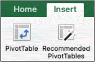
Go to Insert > Recommended PivotTable.
-
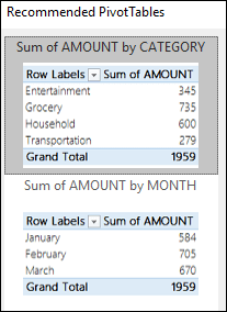
Excel analyzes your data and presents you with several options, like in this example using the household expense data.
-
Select the PivotTable that looks best to you and press OK. Excel will create a PivotTable on a new sheet, and display the PivotTable Fields List

-
Click a cell in the source data or table range.
-
Go to Insert > PivotTable.
-
Excel will display the Create PivotTable dialog with your range or table name selected. In this case, we’re using a table called «tbl_HouseholdExpenses».
-
In the Choose where you want the PivotTable report to be placed section, select New Worksheet, or Existing Worksheet. For Existing Worksheet, select the cell where you want the PivotTable placed.
-
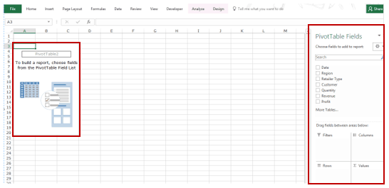
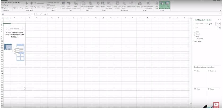
Click OK, and Excel will create a blank PivotTable, and display the PivotTable Fields list.
PivotTable Fields list
In the Field Name area at the top, select the check box for any field you want to add to your PivotTable. By default, non-numeric fields are added to the Row area, date and time fields are added to the Column area, and numeric fields are added to the Values area. You can also manually drag-and-drop any available item into any of the PivotTable fields, or if you no longer want an item in your PivotTable, simply drag it out of the Fields list or uncheck it. Being able to rearrange Field items is one of the PivotTable features that makes it so easy to quickly change its appearance.
PivotTable Fields list
-
Summarize by
By default, PivotTable fields that are placed in the Values area will be displayed as a SUM. If Excel interprets your data as text, it will be displayed as a COUNT. This is why it’s so important to make sure you don’t mix data types for value fields. You can change the default calculation by first clicking on the arrow to the right of the field name, then select the Field Settings option.
Next, change the calculation in the Summarize by section. Note that when you change the calculation method, Excel will automatically append it in the Custom Name section, like «Sum of FieldName», but you can change it. If you click the Number… button, you can change the number format for the entire field.
Tip: Since the changing the calculation in the Summarize by section will change the PivotTable field name, it’s best not to rename your PivotTable fields until you’re done setting up your PivotTable. One trick is to click Replace (on the Edit menu) >Find what > «Sum of«, then Replace with > leave blank to replace everything at once instead of manually retyping.
-
Show data as
Instead of using a calculation to summarize the data, you can also display it as a percentage of a field. In the following example, we changed our household expense amounts to display as a % of Grand Total instead of the sum of the values.
Once you’ve opened the Field Settings dialog, you can make your selections from the Show data as tab.
-
Display a value as both a calculation and percentage.
Simply drag the item into the Values section twice, right-click the value and select Field Settings, then set the Summarize by and Show data as options for each one.
If you add new data to your PivotTable data source, any PivotTables that were built on that data source need to be refreshed. To refresh just one PivotTable you can right-click anywhere in the PivotTable range, then select Refresh. If you have multiple PivotTables, first select any cell in any PivotTable, then on the Ribbon go to PivotTable Analyze > click the arrow under the Refresh button and select Refresh All.
If you created a PivotTable and decide you no longer want it, you can simply select the entire PivotTable range, then press Delete. It won’t have any affect on other data or PivotTables or charts around it. If your PivotTable is on a separate sheet that has no other data you want to keep, deleting that sheet is a fast way to remove the PivotTable.
Data format tips and tricks
-
Use clean, tabular data for best results.
-
Organize your data in columns, not rows.
-
Make sure all columns have headers, with a single row of unique, non-blank labels for each column. Avoid double rows of headers or merged cells.
-
Format your data as an Excel table (select anywhere in your data and then select Insert > Table from the ribbon).
-
If you have complicated or nested data, use Power Query to transform it (for example, to unpivot your data) so it is organized in columns with a single header row.
Need more help?
You can always ask an expert in the Excel Tech Community or get support in the Answers community.
PivotTable Recommendations are a part of the connected experience in Microsoft 365, and analyzes your data with artificial intelligence services. If you choose to opt out of the connected experience in Microsoft 365, your data will not be sent to the artificial intelligence service, and you will not be able to use PivotTable Recommendations. Read the Microsoft privacy statement for more details.
Related articles
Create a PivotChart
Use slicers to filter PivotTable data
Create a PivotTable timeline to filter dates
Create a PivotTable with the Data Model to analyze data in multiple tables
Create a PivotTable connected to Power BI Datasets
Use the Field List to arrange fields in a PivotTable
Change the source data for a PivotTable
Calculate values in a PivotTable
Delete a PivotTable
![]()
Download Article
Step-by-step tutorial for making and editing a pivot table in Excel
![]()
Download Article
- Building the Pivot Table
- Configuring the Pivot Table
- Using the Pivot Table
- Video
- Expert Q&A
- Tips
- Warnings
|
|
|
|
|
|
Trying to make a new pivot table in Microsoft Excel? The process is quick and easy using Excel’s built-in tools. Pivot tables are a great way to create an interactive table for data analysis and reporting. Excel allows you to drag and drop the variables you need in your table to immediately rearrange it. This wikiHow guide will show you how to create pivot tables in Microsoft Excel.
Things You Should Know
- Go to the Insert tab and click «PivotTable» to create a new pivot table.
- Use the PivotTable Fields pane to arrange your variables by row, column, and value.
- Click the drop-down arrow next to fields in the pivot table to sort and filter.
-
1
Open the Excel file where you want to create the pivot table. A pivot table allows you to create tabular reports of data in a spreadsheet. You can also perform calculations without having to input formulas.
- You can also create a pivot table in Excel using an outside data source, such as an Access database.
-
2
Highlight the cells you want to make into a pivot table. Note that the original spreadsheet data will be preserved. Skip this step if you’re going to make the pivot table using an external source of data.
- Make sure your data is formatted correctly. To create a pivot table, you’ll need a dataset that is organized in columns. It should have a single header row.
- Optionally, formatting your original data as a table using Insert > Table will help make sure the formatting is correct.
Advertisement
-
3
Go to the Insert tab and click PivotTable. This will open a new window for creating the pivot table.
- If you are using Excel 2003 or earlier, click the Data menu and select PivotTable and PivotChart Report.
- If you’re using an external source of data, click the drop-down arrow under PivotTable and select From External Data Source. Then click Choose Connection in the new window.
-
4
Select the location for your pivot table and click OK. This will place the new pivot table in the selected location. By default, Excel will place the table on a new worksheet, allowing you to switch back and forth by clicking the tabs at the bottom of the window. You can also choose to place the pivot table on the same sheet as the data, which allows you to pick the cell where you want it to be placed.
- You can later delete the pivot table without losing its data if needed.


Advertisement
-
1
Click the checkbox next to fields you want in the PivotTables Fields pane. This adds the field to your pivot table. Note that fields are what Excel calls the variables in your dataset, based on the headers in the header row.[1]
- Clicking the checkboxes automatically adds the field to a section of the pivot table. Non-numeric fields are placed in the rows section, dates are placed in the columns section, and numeric fields are placed in the values section.
- You can rearrange the fields by dragging them to a different section.
-
2
Add or move a row field. Drag a field from the field list on the right onto the «Row» section of the pivot table pane to add the field to your table.
- For example, your company sells two products: tables and chairs. You have a spreadsheet with the number (Sales) of each product (Product Type) sold in your five stores (Store).
- Drag the Store field from the field list into the Row Fields section of the pivot table. Your list of stores will appear, each as its own row.
-
3
Add a value field. Drag a field from the field list on the right onto the «Values» section of the pivot table pane to add the field to your table. The values will be calculated and organized based on the rows and columns you select.
- Continuing our example: Click and drag the Sales field into the Value Fields section of the pivot table. You will see your table display the sales information for each of your stores.
-
4
Add or move a column field. Drag a field from the field list on the right onto the «Column» section of the pivot table pane to add the column field to your table. This is used to separate your data by different categories or dates.
- Continuing our example, you could move Product Type to the columns section to see the product sales data for each store.
-
5
Add multiple fields to a section. Pivot tables allow you to add multiple fields to each section, displaying more information on the table or further subdividing the data.
- Using the above example, say you make several types of tables and several types of chairs. Your data notes whether the item is a table or chair (Product Type), but also the exact model of the table or chair sold (Model).
- Drag the Model field onto the Column Fields section. The columns will now display the breakdown of sales per model and overall type. You can change the order that these labels are displayed by clicking the arrow button next to the field in the boxes in the lower-right corner of the window. Select Move Up or Move Down to change the order.
-
6
Change the way data is displayed. You can change the way values are displayed by following these steps:
- Click the arrow icon next to a value in the Values box.
- Select Value Field Settings to change the way the values are calculated.
- For example, you could display the average value instead of a sum.
- You can add the same field to the Value box multiple times to take advantage of this. In the above example, the sales total for each store is displayed. By adding the Sales field again, you can change the value settings to show the second Sales as a percentage of total sales.
-
7
Learn some of the ways that values can be manipulated. When changing the ways values are calculated, you have several options to choose from depending on your needs.
- Sum — This is the default for value fields. Excel will total all of the values in the selected field.
- Count — This will count the number of cells that contain data in the selected field.
- Average — This will take the average of all of the values in the selected field.
-
8
Click the drop-down arrow next to a field to add a filter and sort data. Note that this is next to the field header in the pivot table, not in the pivot table editor pane. Adding a filter allows you to display only certain data given the criteria you select. Sorting the data changes the order that it appears in the pivot table.


Advertisement
-
1
Update your pivot table. Your pivot table will automatically update as you modify the data in the spreadsheet. This can be great for monitoring your spreadsheets and tracking changes.
- You can also manually update the pivot table by clicking Refresh in the PivotTable Analyze tab.
-
2
Change your pivot table around. Pivot tables are easy to edit using the editing pane. Try dragging different fields to different locations to come up with a pivot table that meets your exact needs.
- This is where the pivot table gets its name. Moving the data to different locations is known as «pivoting» as you are changing the direction that the data is displayed.
-
3
Create a pivot chart. You can use a pivot chart to show dynamic visual reports. Your Pivot Chart can be created directly from your completed pivot table.
- Click PivotChart in the «Tools» section of the PivotTable Analyze tab to make a pivot chart.


Advertisement
Add New Question
-
Question
I have created pivot tables in Excel 2020. I have selected in Design Totals to show Column and row totals but row totals will not show. Any advice please?

Kyle Smith is a wikiHow Technology Writer, learning and sharing information about the latest technology. He has presented his research at multiple engineering conferences and is the writer and editor of hundreds of online electronics repair guides. Kyle received a BS in Industrial Engineering from Cal Poly, San Luis Obispo.
wikiHow Technology Writer
Expert Answer
You can try using the PivotTable Options menu to resolve this issue. Go to the PivotTable Analyze tab > click the drop-down arrow under the PivotTable button > click Options > go to the Totals & Filters tab > check the box next to «Show grand totals for rows.»
-
Question
How do I change a name in a field/column in an existing pivot table without changing the field before/after the field requiring the update?
Kyle Smith is a wikiHow Technology Writer, learning and sharing information about the latest technology. He has presented his research at multiple engineering conferences and is the writer and editor of hundreds of online electronics repair guides. Kyle received a BS in Industrial Engineering from Cal Poly, San Luis Obispo.
wikiHow Technology Writer
Expert Answer
You can change a field name by right-clicking a value of the field in the pivot table > select Field Settings > and enter a new name in the «Custom Name» section.
-
Question
Why doesn’t my pivot table show the changes I made to the base file?
There could be couple of reasons: the base file could be missing from original location, or you did not save the changes properly in the base file. Also, remember to save your pivot table before you can expect to see any changes reflected.

See more answers
Ask a Question
200 characters left
Include your email address to get a message when this question is answered.
Submit
Advertisement
wikiHow Video: How to Create Pivot Tables in Excel
-
If you use the Import Data command from the Data menu, you have more options on how to import data ranging from Office Database connections, Excel files, Access databases, Text files, ODBC DSNs, webpages, OLAP and XML/XSL. You can then use your data as you would an Excel list.
-
If you are using an AutoFilter (Under «Data», «Filter»), disable this when creating the pivot table. It is okay to re-enable it after you have created the pivot table.
-
In addition to pivot tables, another powerful tool in Excel is the Solver function.
Thanks for submitting a tip for review!
Advertisement
-
If you are using data in an existing spreadsheet, make sure that the range that you select has a unique column name at the top of each column of data.
Advertisement
References
About This Article
Article SummaryX
A pivot table is an interactive table that lets you group and summarize data in a concise, tabular format. To create a pivot table, click the Insert tab, and then click the PivotTable icon on the toolbar. You can enter your data range manually, or quickly select it by dragging the mouse cursor across all cells in the range, including the labeled column headers. Or, if the data is in an external database, select Use an external data source, and then choose that database and range. Your new pivot table will be placed on the active worksheet by default, but you can change the sheet name and range under «»Existing Worksheet»» to put it elsewhere, or select New Worksheet to place it on its own brand new sheet. Click OK to place your pivot table on the selected sheet.
You’ll use the Pivot Table Fields bar on the right to lay out your table in columns and rows. Drag fields to the Columns and Rows areas, and then drag fields that represent values to the Values area. Adding fields to the Filters area lets you filter your table by the type of data in that field. You can add multiple data fields to any of these sections, and move things around until they look the way you’d like. Once you’ve created your table, you can click the PivotTable Analyze tab to view and manage more settings, or the Design tab to customize its color and style.
Did this summary help you?
Thanks to all authors for creating a page that has been read 2,133,227 times.
Reader Success Stories
-

«What helped me most with my questions were the sequential steps and explanations on what to do and how to do it. …» more
Is this article up to date?
The pivot table is one of Microsoft Excel’s most powerful — and intimidating — functions. Pivot tables can help you summarize and make sense of large data sets. However, they also have a reputation for being complicated.

The good news is that learning how to create a pivot table in Excel is much easier than you may believe.
We’re going to walk you through the process of creating a pivot table and show you just how simple it is. First, though, let’s take a step back and make sure you understand exactly what a pivot table is, and why you might need to use one.
What is a pivot table?
What are pivot tables used for?
How to Create a Pivot Table
Pivot Table Examples
![Download 10 Excel Templates for Marketers [Free Kit]](https://no-cache.hubspot.com/cta/default/53/9ff7a4fe-5293-496c-acca-566bc6e73f42.png)
What is a pivot table?
A pivot table is a summary of your data, packaged in a chart that lets you report on and explore trends based on your information. Pivot tables are particularly useful if you have long rows or columns that hold values you need to track the sums of and easily compare to one another.
In other words, pivot tables extract meaning from that seemingly endless jumble of numbers on your screen. And more specifically, it lets you group your data in different ways so you can draw helpful conclusions more easily.
The «pivot» part of a pivot table stems from the fact that you can rotate (or pivot) the data in the table to view it from a different perspective. To be clear, you’re not adding to, subtracting from, or otherwise changing your data when you make a pivot. Instead, you’re simply reorganizing the data so you can reveal useful information.
What are pivot tables used for?
If you’re still feeling a bit confused about what pivot tables actually do, don’t worry. This is one of those technologies that are much easier to understand once you’ve seen it in action.
The purpose of pivot tables is to offer user-friendly ways to quickly summarize large amounts of data. They can be used to better understand, display, and analyze numerical data in detail.
With this information, you can help identify and answer unanticipated questions surrounding the data.
Here are seven hypothetical scenarios where a pivot table could be helpful.
1. Comparing Sales Totals of Different Products
Let’s say you have a worksheet that contains monthly sales data for three different products — product 1, product 2, and product 3. You want to figure out which of the three has been generating the most revenue.
One way would be to look through the worksheet and manually add the corresponding sales figure to a running total every time product 1 appears. The same process can then be done for product 2, and product 3 until you have totals for all of them. Piece of cake, right?
Imagine, now, that your monthly sales worksheet has thousands upon thousands of rows. Manually sorting through each necessary piece of data could literally take a lifetime.
With pivot tables, you can automatically aggregate all of the sales figures for product 1, product 2, and product 3 — and calculate their respective sums — in less than a minute.
 Image source
2. Showing Product Sales as Percentages of Total Sales
Pivot tables inherently show the totals of each row or column when created. That’s not the only figure you can automatically produce, however.
Let’s say you entered quarterly sales numbers for three separate products into an Excel sheet and turned this data into a pivot table. The pivot table automatically gives you three totals at the bottom of each column — having added up each product’s quarterly sales.
But what if you wanted to find the percentage these product sales contributed to all company sales, rather than just those products’ sales totals?
With a pivot table, instead of just the column total, you can configure each column to give you the column’s percentage of all three column totals.
Let’s say three products totaled $200,000 in sales. The first product made $45,000, you can edit a pivot table to instead say this product contributed 22.5% of all company sales.
To show product sales as percentages of total sales in a pivot table, simply right-click the cell carrying a sales total and select Show Values As > % of Grand Total.
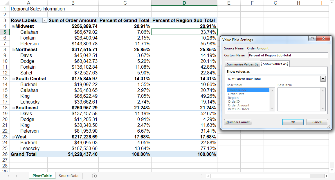 Image source
3. Combining Duplicate Data
In this scenario, you’ve just completed a blog redesign and had to update many URLs. Unfortunately, your blog reporting software didn’t handle the change well and split the «view» metrics for single posts between two different URLs.
In your spreadsheet, you now have two separate instances of each individual blog post. To get accurate data, you need to combine the view totals for each of these duplicates.
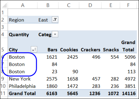 Image source
Instead of having to manually search for and combine all the metrics from the duplicates, you can summarize your data (via pivot table) by blog post title.
Voilà, the view metrics from those duplicate posts will be aggregated automatically.
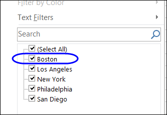 Image source
4. Getting an Employee Headcount for Separate Departments
Pivot tables are helpful for automatically calculating things that you can’t easily find in a basic Excel table. One of those things is counting rows that all have something in common.
For instance, let’s say you have a list of employees in an Excel sheet. Next to the employees’ names are the respective departments they belong to. You can create a pivot table from this data that shows you each department’s name and the number of employees that belong to those departments.
The pivot table’s automated functions effectively eliminate your task of sorting the Excel sheet by department name and counting each row manually.
5. Adding Default Values to Empty Cells
Not every dataset you enter into Excel will populate every cell. If you’re waiting for new data to come in, you might have lots of empty cells that look confusing or need further explanation.
That’s where pivot tables come in.
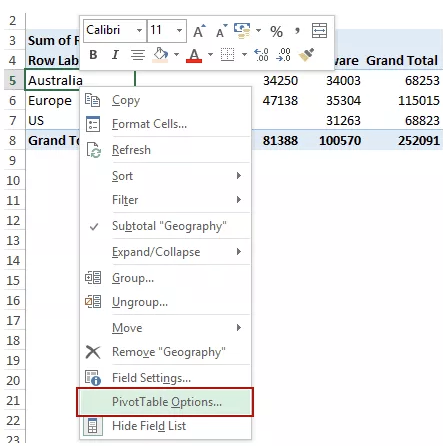 Image source
You can easily customize a pivot table to fill empty cells with a default value, such as $0, or TBD (for «to be determined»). For large data tables, being able to tag these cells quickly is a valuable feature when many people are reviewing the same sheet.
To automatically format the empty cells of your pivot table, right-click your table and click PivotTable Options.
In the window that appears, check the box labeled Empty Cells As and enter what you’d like displayed when a cell has no other value.
 Image source
- Enter your data into a range of rows and columns.
- Sort your data by a specific attribute.
- Highlight your cells to create your pivot table.
- Drag and drop a field into the «Row Labels» area.
- Drag and drop a field into the «Values» area.
- Fine-tune your calculations.
Now that you have a better sense of what pivot tables can be used for, let’s get into the nitty-gritty of how to actually create one.
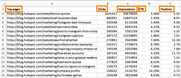
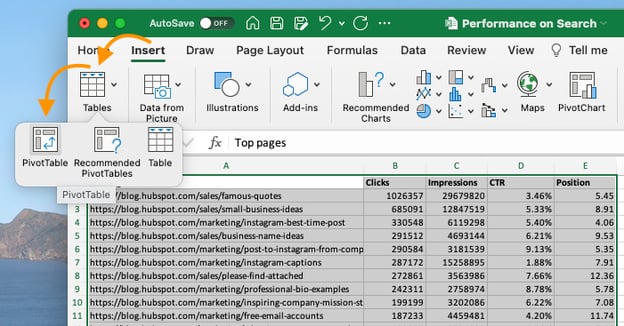
Step 1. Enter your data into a range of rows and columns.
Every pivot table in Excel starts with a basic Excel table, where all your data is housed. To create this table, simply enter your values into a specific set of rows and columns. Use the topmost row or the topmost column to categorize your values by what they represent.
For example, to create an Excel table of blog post performance data, you might have:
- A column listing each «Top Pages.»
- A column listing each URL’s «Clicks.»
- A column listing each post’s «Impressions.»
We’ll be using that example in the steps that follow.
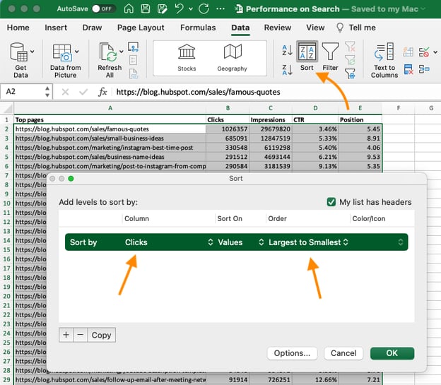
Step 2. Sort your data by a specific attribute.
Once you’ve entered all your data into your Excel sheet, you’ll want to sort your data by attribute. This will make your information easier to manage once it becomes a pivot table.
To sort your data, click the Data tab in the top navigation bar and select the Sort icon underneath it. In the window that appears, you can sort your data by any column you want and in any order.
For example, to sort your Excel sheet by «Views to Date,» select this column title under Column and then select whether you want to order your posts from smallest to largest, or from largest to smallest.
Select OK on the bottom-right of the Sort window.
Now, you’ve successfully reordered each row of your Excel sheet by the number of views each blog post has received.
Step 3. Highlight your cells to create your pivot table.
Once you’ve entered and sorted your data, highlight the cells you’d like to summarize in a pivot table. Click Insert along the top navigation, and select the PivotTable icon.
You can also click anywhere in your worksheet, select «PivotTable,» and manually enter the range of cells you’d like included in the PivotTable.
This opens an options box. Here you can select whether or not to launch this pivot table in a new worksheet or keep it in the existing worksheet, in addition to setting your cell range.
If you open a new sheet, you can navigate to and away from it at the bottom of your Excel workbook. Once you’ve chosen, click OK.
Alternatively, you can highlight your cells, select Recommended PivotTables to the right of the PivotTable icon, and open a pivot table with pre-set suggestions for how to organize each row and column.
Note: If using an earlier version of Excel, «PivotTables» may be under Tables or Data along the top navigation, rather than «Insert.» In Google Sheets, you can create pivot tables from the Data dropdown along the top navigation.
Step 4. Drag and drop a field into the «Row Labels» area.
After you’ve completed Step 3, Excel will create a blank pivot table for you.
Your next step is to drag and drop a field — labeled according to the names of the columns in your spreadsheet — into the Row Labels area. This will determine what unique identifier the pivot table will organize your data by.
For example, let’s say you want to organize a bunch of blogging data by post title. To do that, you’d simply click and drag the “Top pages” field to the «Row Labels» area.
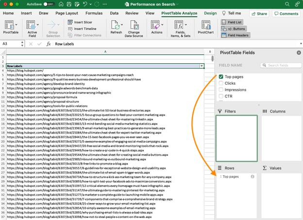
Note: Your pivot table may look different depending on which version of Excel you’re working with. However, the general principles remain the same.
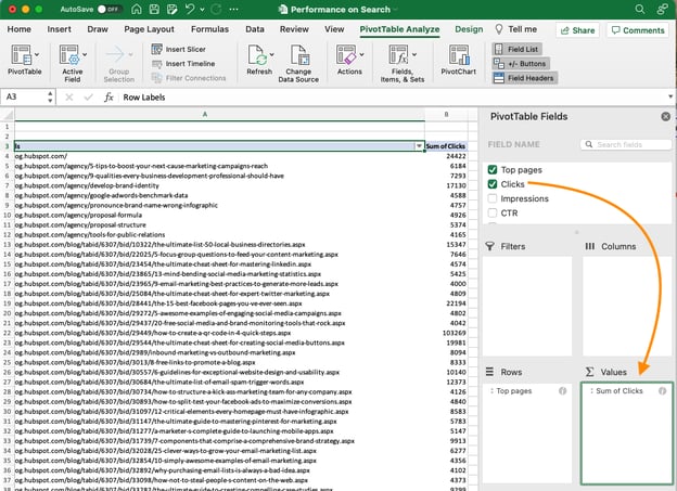
Step 5. Drag and drop a field into the «Values» area.
Once you’ve established how you’re going to organize your data, your next step is to add in some values by dragging a field into the Values area.
Sticking with the blogging data example, let’s say you want to summarize blog post views by title. To do this, you’d simply drag the «Views» field into the Values area.
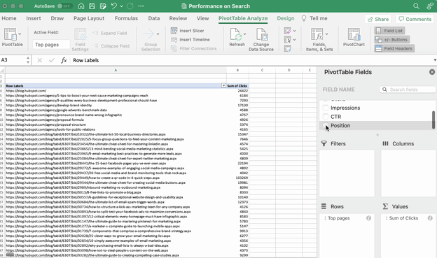
Step 6. Fine-tune your calculations.
The sum of a particular value will be calculated by default, but you can easily change this to something like average, maximum, or minimum depending on what you want to calculate.
On a Mac, you can do this by clicking on the small i next to a value in the «Values» area, selecting the option you want, and clicking «OK.» Once you’ve made your selection, your pivot table will be updated accordingly.
If you’re using a PC, you’ll need to click on the small upside-down triangle next to your value and select Value Field Settings to access the menu.
When you’ve categorized your data to your liking, save your work and use it as you please.
Pivot Table Examples
From managing money to keeping tabs on your marketing effort, pivot tables can help you keep track of important data. The possibilities are endless!
See three pivot table examples below to keep you inspired.
1. Creating a PTO Summary and Tracker
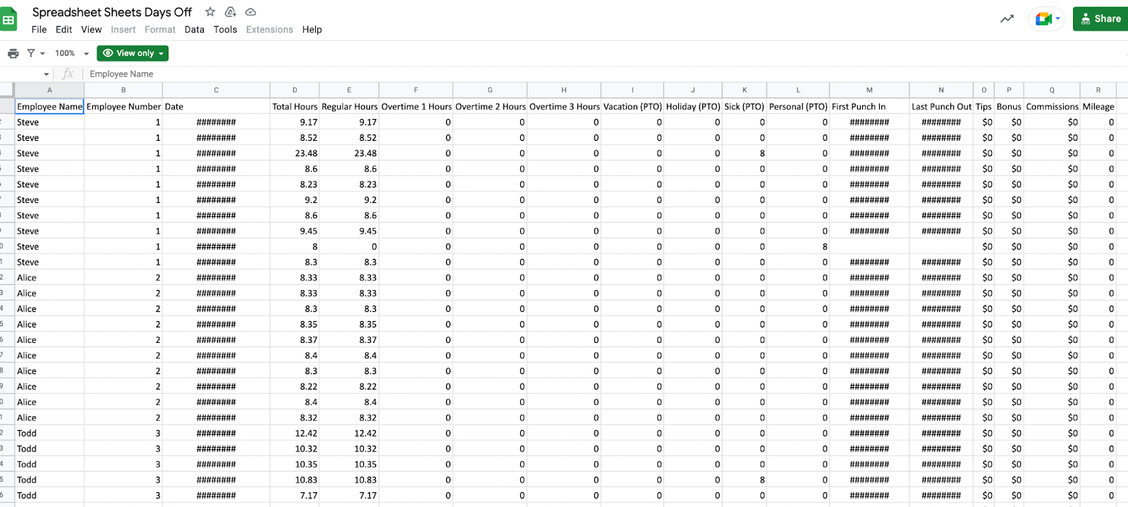 Image source
If you’re in HR, running a business, or leading a small team, managing employees’ vacations is essential. This pivot allows you to seamlessly track this data.
All you need to do is import your employee’s identification data along with the following data:
- Sick time.
- Hours of PTO.
- Company holidays.
- Overtime hours.
- Employee’s regular number of hours.
From there, you can sort your pivot table by any of these categories.
2. Building a Budget
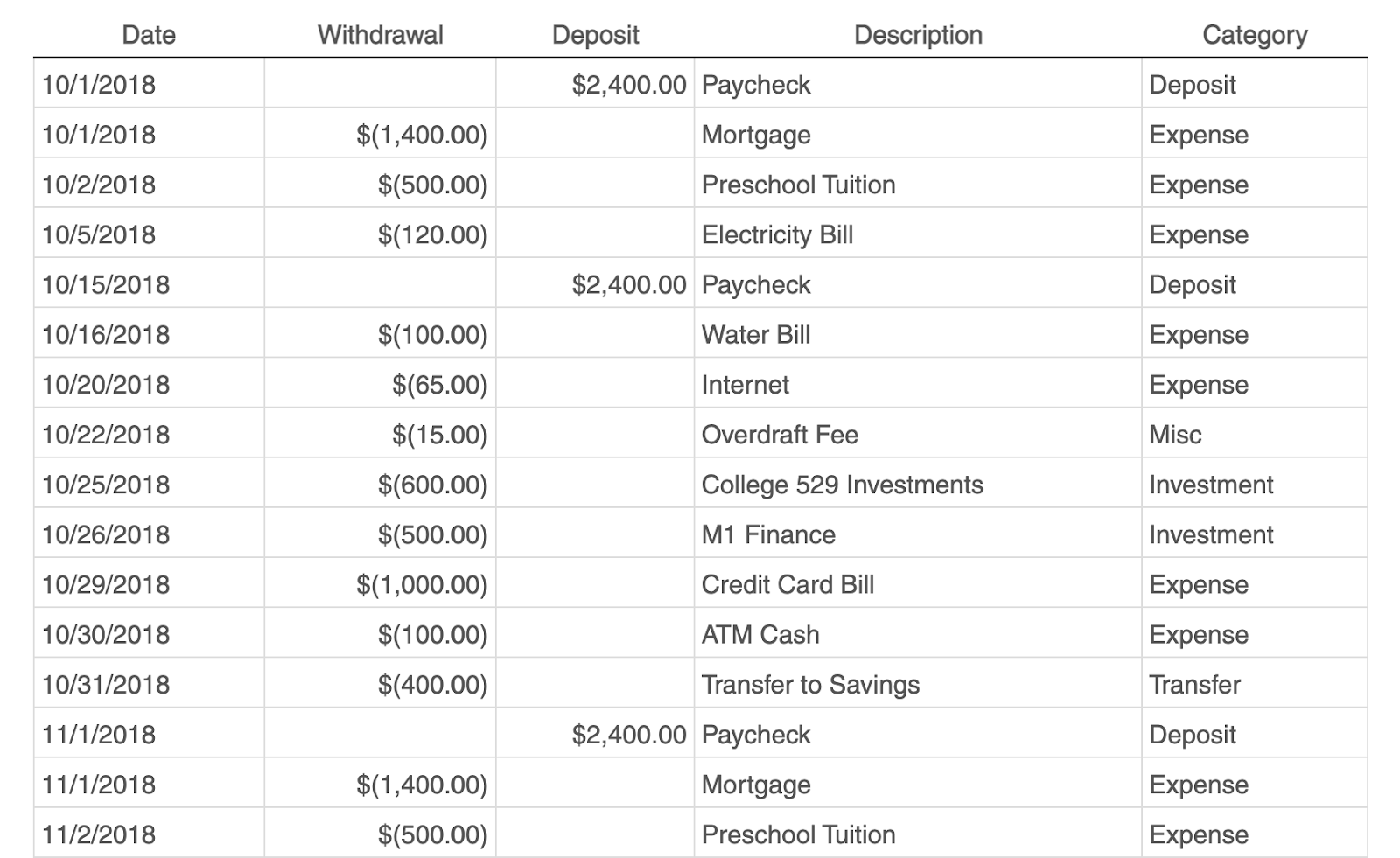 Image source
Whether you’re running a project or just managing your own money, pivot tables are an excellent tool for tracking spend.
The simplest budget just requires the following categories:
- Date of transaction
- Withdrawal/Expenses
- Deposit/Income
- Description
- Any overarching categories (like paid ads or contractor fees)
With this information, you can see your biggest expenses and brainstorm ways to save.
3. Tracking Your Campaign Performance
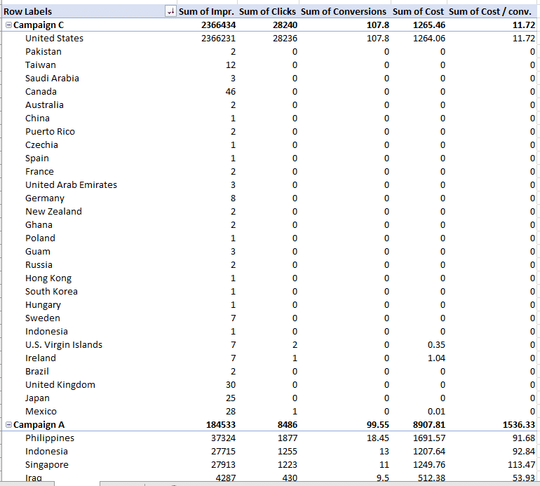 Image source
Pivot tables can help your team assess the performance of your marketing campaigns.
In this example, campaign performance is split by region. You can easily which country had the highest conversions during different campaigns.
This can help you identify tactics that perform well in each region and where advertisements need to be changed.
Digging Deeper With Pivot Tables
You’ve now learned the basics of pivot table creation in Excel. With this understanding, you can figure out what you need from your pivot table and find the solutions you’re looking for.
For example, you may notice that the data in your pivot table isn’t sorted the way you’d like. If this is the case, Excel’s Sort function can help you out. Alternatively, you may need to incorporate data from another source into your reporting, in which case the VLOOKUP function could come in handy.
Editor’s note: This post was originally published in December 2018 and has been updated for comprehensiveness.

If you are reading this tutorial, there is a big chance you have heard of (or even used) the Excel Pivot Table. It’s one of the most powerful features in Excel (no kidding).
The best part about using a Pivot Table is that even if you don’t know anything in Excel, you can still do pretty awesome things with it with a very basic understanding of it.
Let’s get started.
Click here to download the sample data and follow along.
What is a Pivot Table and Why Should You Care?
A Pivot Table is a tool in Microsoft Excel that allows you to quickly summarize huge datasets (with a few clicks).
Even if you’re absolutely new to the world of Excel, you can easily use a Pivot Table. It’s as easy as dragging and dropping rows/columns headers to create reports.
Suppose you have a dataset as shown below:
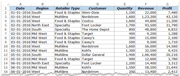
This is sales data that consists of ~1000 rows.
It has the sales data by region, retailer type, and customer.
Now your boss may want to know a few things from this data:
- What were the total sales in the South region in 2016?
- What are the top five retailers by sales?
- How did The Home Depot’s performance compare against other retailers in the South?
You can go ahead and use Excel functions to give you the answers to these questions, but what if suddenly your boss comes up with a list of five more questions.
You’ll have to go back to the data and create new formulas every time there is a change.
This is where Excel Pivot Tables comes in really handy.
Within seconds, a Pivot Table will answer all these questions (as you’ll learn below).
But the real benefit is that it can accommodate your finicky data-driven boss by answering his questions immediately.
It’s so simple, you may as well take a few minutes and show your boss how to do it himself.
Hopefully, now you have an idea of why Pivot Tables are so awesome. Let’s go ahead and create a Pivot Table using the data set (shown above).
Inserting a Pivot Table in Excel
Here are the steps to create a pivot table using the data shown above:
As soon as you click OK, a new worksheet is created with the Pivot Table in it.
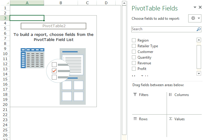
While the Pivot Table has been created, you’d see no data in it. All you’d see is the Pivot Table name and a single line instruction on the left, and Pivot Table Fields on the right.
Now before we jump into analyzing data using this Pivot Table, let’s understand what are the nuts and bolts that make an Excel Pivot Table.
Also read: 10 Excel Pivot Table Keyboard Shortcuts
The Nuts & Bolts of an Excel Pivot Table
To use a Pivot Table efficiently, it’s important to know the components that create a pivot table.
In this section, you’ll learn about:
- Pivot Cache
- Values Area
- Rows Area
- Columns Area
- Filters Area
Pivot Cache
As soon as you create a Pivot Table using the data, something happens in the backend. Excel takes a snapshot of the data and stores it in its memory. This snapshot is called the Pivot Cache.
When you create different views using a Pivot Table, Excel does not go back to the data source, rather it uses the Pivot Cache to quickly analyze the data and give you the summary/results.
The reason a pivot cache gets generated is to optimize the pivot table functioning. Even when you have thousands of rows of data, a pivot table is super fast in summarizing the data. You can drag and drop items in the rows/columns/values/filters boxes and it will instantly update the results.
Note: One downside of pivot cache is that it increases the size of your workbook. Since it’s a replica of the source data, when you create a pivot table, a copy of that data gets stored in the Pivot Cache.
Read More: What is Pivot Cache and How to Best Use It.
Values Area
The Values Area is what holds the calculations/values.
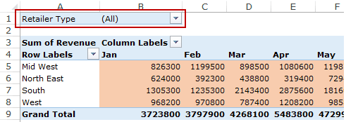
Based on the data set shown at the beginning of the tutorial, if you quickly want to calculate total sales by region in each month, you can get a pivot table as shown below (we’ll see how to create this later in the tutorial).
The area highlighted in orange is the Values Area.
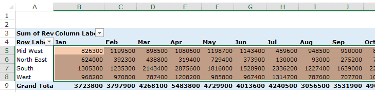
In this example, it has the total sales in each month for the four regions.
Rows Area
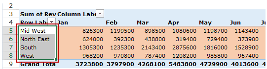
The headings to the left of the Values area makes the Rows area.
In the example below, the Rows area contains the regions (highlighted in red):
Columns Area
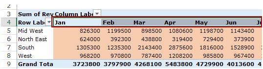
The headings at the top of the Values area makes the Columns area.
In the example below, Columns area contains the months (highlighted in red):
Filters Area
Filters area is an optional filter that you can use to further drill down in the data set.
For example, if you only want to see the sales for Multiline retailers, you can select that option from the drop down (highlighted in the image below), and the Pivot Table would update with the data for Multiline retailers only.
Analyzing Data Using the Pivot Table
Now, let’s try and answer the questions by using the Pivot Table we have created.
Click here to download the sample data and follow along.
To analyze data using a Pivot Table, you need to decide how you want the data summary to look in the final result. For example, you may want all the regions in the left and the total sales right next to it. Once you have this clarity in mind, you can simply drag and drop the relevant fields in the Pivot Table.
In the Pivot Tabe Fields section, you have the fields and the areas (as highlighted below):
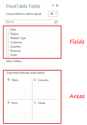
The Fields are created based on the backend data used for the Pivot Table. The Areas section is where you place the fields, and according to where a field goes, your data is updated in the Pivot Table.
It’s a simple drag and drop mechanism, where you can simply drag a field and put it in one of the four areas. As soon as you do this, it will appear in the Pivot Table in the worksheet.
Now let’s try and answer the questions your manager had using this Pivot Table.
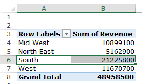
Q1: What were the total sales in the South region?
Drag the Region field in the Rows area and the Revenue field in the Values area. It would automatically update the Pivot Table in the worksheet.
Note that as soon as you drop the Revenue field in the Values area, it becomes Sum of Revenue. By default, Excel sums all the values for a given region and shows the total. If you want, you can change this to Count, Average, or other statistics metrics. In this case, the sum is what we needed.
The answer to this question would be 21225800.
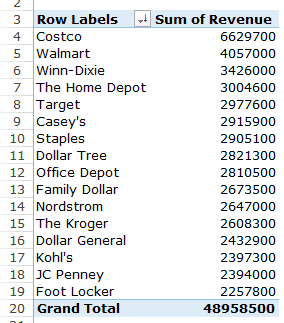
Q2 What are the top five retailers by sales?
Drag the Customer field in the Row area and Revenue field in the values area. In case, there are any other fields in the area section and you want to remove it, simply select it and drag it out of it.
You’ll get a Pivot Table as shown below:
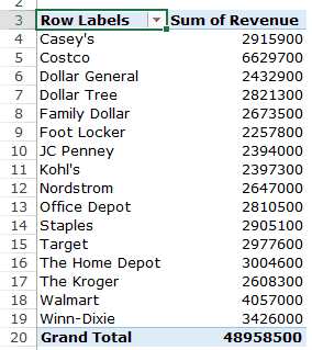
Note that by default, the items (in this case the customers) are sorted in an alphabetical order.
To get the top five retailers, you can simply sort this list and use the top five customer names. To do this:
This will give you a sorted list based on total sales.
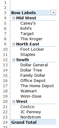
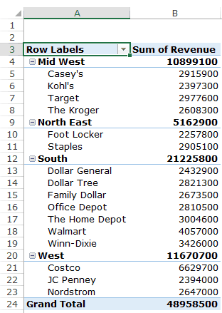
Q3: How did The Home Depot’s performance compare against other retailers in the South?
You can do a lot of analysis for this question, but here let’s just try and compare the sales.
Drag the Region Field in the Rows area. Now drag the Customer field in the Rows area below the Region field. When you do this, Excel would understand that you want to categorize your data first by region and then by customers within the regions. You’ll have something as shown below:
Now drag the Revenue field in the Values area and you’ll have the sales for each customer (as well as the overall region).
You can sort the retailers based on the sales figures by following the below steps:
- Right-click on a cell that has the sales value for any retailer.
- Go to Sort –> Sort Largest to Smallest.
This would instantly sort all the retailers by the sales value.
Now you can quickly scan through the South region and identify that The Home Depot sales were 3004600 and it did better than four retailers in the South region.
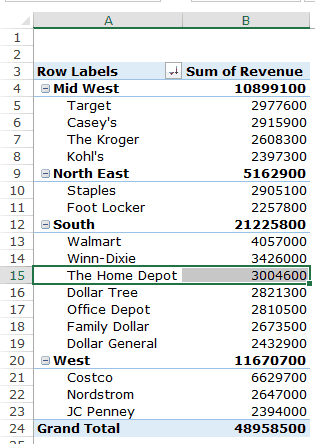
Now there are more than one ways to skin the cat. You can also put the Region in the Filter area and then only select the South Region.
Click here to download the sample data.
I hope this tutorial gives you a basic overview of Excel Pivot Tables and helps you in getting started with it.
Here are some more Pivot Table Tutorials you may like:
- Preparing Source Data For Pivot Table.
- How to Apply Conditional Formatting in a Pivot Table in Excel.
- How to Group Dates in Pivot Tables in Excel.
- How to Group Numbers in Pivot Table in Excel.
- How to Filter Data in a Pivot Table in Excel.
- Using Slicers in Excel Pivot Table.
- How to Replace Blank Cells with Zeros in Excel Pivot Tables.
- How to Add and Use an Excel Pivot Table Calculated Fields.
- How to Refresh Pivot Table in Excel.
Home > Microsoft Excel > How to Create a Pivot Table in Excel? — The Easiest guide
If you ask anyone with decent experience in using Excel, about the most useful Excel feature, they will vouch for the Excel Pivot Table. It is one of the most searched Excel features on the internet, and for good reason.
Related:
Creating A Dynamic Pivot Chart Title Using Slicers
Using Getpivotdata In Excel
Dashboards In Excel Using Pivot Tables, Pivot Charts And Slicers
In this guide, let’s see what makes the Pivot table one of the most popular and powerful Excel features.
This guide covers
Table Of Contents
- What is a Pivot Table?
- What is the use of a Pivot Table in Excel?
- How does an Excel Pivot Table work?
- How to Create a Pivot Table in Excel?
- Step 1: Turn the Data Range into a Table
- Step 2: Open the Create Pivot Table Wizard
- Step 3: Select the Source Table or Range for the Pivot Table
- Step 4: Set the Location of the Pivot Table
- How to Add Data to an Excel Pivot Table?
- Four Quadrants
- Values:
- Rows:
- Columns:
- Filters:
- Value Field Settings
- Analyse data using Pivot Table
- Sales Values across Months
- Sales Values across months in Each branch.
- Sales Values across months in Each branch for each department.
- What are the Benefits of Pivot Tables?
- FAQs
- What is the use of a Pivot Table in Excel?
- What is a Pivot Table formula?
- Let’s wrap up
What is a Pivot Table?
Microsoft describes a Pivot Table in Excel (or PivotTable if you’re using the trademarked function name!) as “an interactive way to quickly summarize large amounts of data”. It’s a pretty good description.
What is the use of a Pivot Table in Excel?
The Excel Pivot Table function is an essential part of data analysis in Excel. Before the Pivot Table came along you’d need multiple functions tied together in a complicated and convoluted way to perform the same action that just takes a few clicks in a Pivot Table.
To say they revolutionised the way the average Excel user performs data analysis is an understatement. They are such a big deal that they have their own Wikipedia page.
For the end-user, Pivot Tables are remarkably simple to use and easy to learn. There are hundreds of brilliant articles on how to create your first Pivot Table as well as some excellent lessons on YouTube.
We’re going to contribute by showing you some of our highest rated videos that teach you how to create a Pivot Table in Excel.
If for any reason you don’t get it the first time, don’t worry, we’ve included multiple Pivot Table tutorials to help you master this essential skill.
If you have an hour to dedicate to a Pivot Table tutorial, then start with the video below. This is a recording of a live class we held in 2019 that takes you through everything you need to know to start analysing your data using Pivot Tables. These live classes are all free as part of a Simon Sez IT membership.
If that’s too much, scroll down and we have some other, shorter videos taken straight from our Excel courses.
How does an Excel Pivot Table work?
All Pivot Tables start life as a boring old range of data. But once you create a Pivot Table, Excel takes a quick look at the data and stores it in its cache.
This is called the Pivot cache and it is responsible for the super fast calculation of summaries that Pivot Tables are known for.
Each time you add or remove data from the Excel Pivot Table, Excel does not deal with the source data, rather it uses this Pivot Cache as a quick shortcut.
Also Read:
Introduction To Power Pivot and Power Query In Excel
Getting Started With Power Pivot: Advanced Excel
Excel Crash Course – Learn Pivot Tables In 1 Hour
How to Create a Pivot Table in Excel?
Step 1: Turn the Data Range into a Table
You can create a Pivot Table in Excel from a range but we strongly recommend that you turn your range into a table as this makes it a lot simpler to add or remove data later on.
For example:
A few golden rules about your data range or table before you create an Excel Pivot Table with it:
- Every column should have a header. If one is missing, you won’t be able to create a Pivot Table.
- There should be no empty rows. There can be the odd empty cell, but no full empty rows. This can mess up a few things.
Step 2: Open the Create Pivot Table Wizard
Once you’ve turned your range into a table (use Ctrl-T to do this quickly!) you then need to select a cell in that table, go to Insert on the ribbon and select Pivot Table on the far left.
This brings up the Create Pivot Table Wizard where you can start selecting your Pivot Table options.
Step 3: Select the Source Table or Range for the Pivot Table
The first option you’ll notice is that Excel is asking you to select the table or range. Because we have already created a table and we were clicked into that table when we chose to insert the Pivot Table, Excel has done the hard work for us and has selected that table as our range of data.
Step 4: Set the Location of the Pivot Table
Select whether you create your Pivot Table in a new or an existing worksheet. Once you hit OK, you’ve created your first Pivot Table. Hurray!
What you’ll see next is a blank table to the left with a set of options on your right. These options are the Pivot Table fields and this is where the magic starts to happen. I’ll show you how to do this in the next section.
How to Add Data to an Excel Pivot Table?
Using the Pivot Table Fields panel you can now start to manipulate your data.
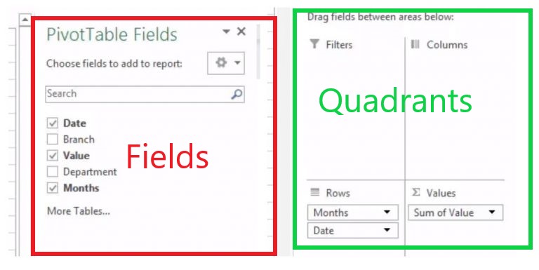
Four Quadrants
A pivot table is based on these four quadrants:
- Filters
- Columns
- Rows
- Values
We’ll see what each of these quadrants mean in a minute.
These four quadrants are the key to manipulating the data in your Pivot Table. You can now start to drag the values at the top of the Excel Pivot Table Fields section into the quadrants below.
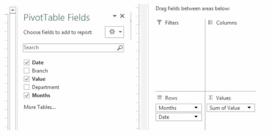
Values:
The values quadrant is what decides the type and value of calculations that the Pivot Table should display. It is the meat of a Pivot Table so to speak.
In the following image, the area bordered in red is the Values area in a Pivot Table.
Rows:
The rows quadrant is what decides the rows that the Pivot Table should display. The Rows are used to slice the data in a suitable way that we are looking for.
For example, you want to look at the total sales that occurred in different months. For this, you need to drag Months in the Rows quadrant.
In the following image, the area bordered in green is the Rows area of a Pivot Table.
Columns:
The columns quadrant is what decides the columns that the Pivot Table should display. That is columns are used to further dice the data into a suitable format.
For example, you want to look at the total sales that occurred in different months across different departments. For this, you need to drag Months in the Rows quadrant and further drag Departments into the Columns quadrant.
In the following image, the area bordered in blue is the Columns area of a Pivot Table.

Filters:
The filters quadrant is optional and is used to further drill down your Pivot Table. For example, you may want to look only at the sales value of the Detroit Branch.
This can be done by dragging the Branch field into the filter quadrant. Now, you can select the branch you are looking for from the drop-down list and view only its data.
Value Field Settings
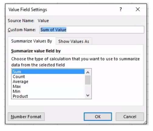
How do you change what’s happening in your value field away from displaying the sum? Simple, you need Value Field Settings.
To access these select any value in your Pivot Table, go to analyze on the ribbon and select “Field Settings”. Alternatively, click the little down arrow in the value quadrant and select “Value Field Settings”.
This brings up the options you have in relation to your values. You can average instead of sum, you can count or use Min or Max. You can then select how you show the values including adding some calculations and changing the number format.
Analyse data using Pivot Table
Depending on which quadrant you pick, the table will format differently so there are a few rules to stick to:
- Numbers nearly always go in the Values quadrant. This allows you to perform calculations, summaries, averages etc. all from within your Pivot Table.
- Dates often go in the Rows column because…
- Anything you put in the rows column will become the row headings, anything in the columns quadrant will become column headings so for ease of use put the data with more options in the Rows column (it’s easier to scroll down rather than across for ages).
- The Filters quadrant does what you’d expect, it applies a filter to the entire dataset. Super useful if you just want to show something specific.
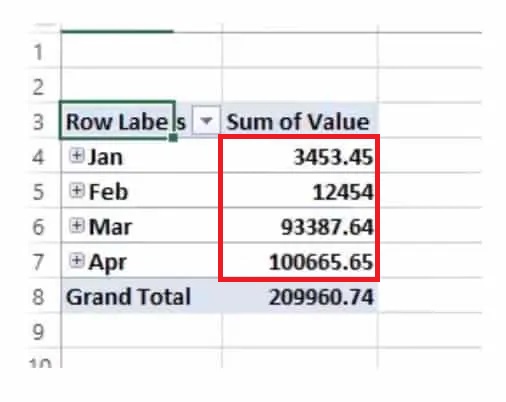
Sales Values across Months
Say you have dates in your rows quadrant and a set of corresponding values in your values quadrant. Excel will automatically do a couple of things.
- It will condense the dates into months, quarters or years (depending on the data set).
- It will sum the values in the values field.
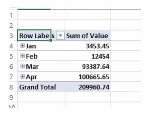
This is the Pivot Table starting to work. From your dataset, it’s now summarising that data by month for you. All within a few clicks.
Of course, you may not want that exact data and you may not want to add it together. The amazing thing about the Excel Pivot Table function is just how flexible it is.
You can drag and drop, remove and change the data within those quadrants as much as you want and you’ll start to see just how powerful Pivot Tables are.
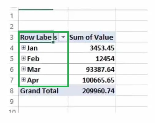
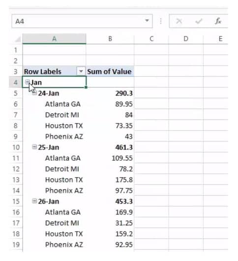
Sales Values across months in Each branch.
The data in our example is sales data. Above we’re seeing sales by month which is useful. But what if we wanted to see sales by branch and by date?
Easy, we just drop the branch data into the rows column, under the date and we get a breakdown of that as well:
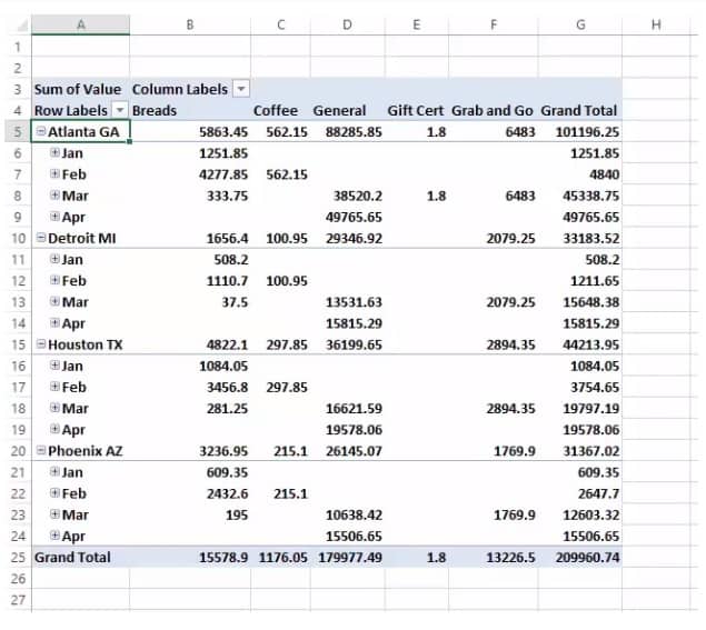
Sales Values across months in Each branch for each department.
If we wanted to get even more detail we could then add the departments to the column data and we’d see a summary of sales by branch, by the department and by date! You can quickly see that with very little effort on our part we can now draw really meaningful insight from our dataset:
What are the Benefits of Pivot Tables?
All that an Excel Pivot table does is help you effortlessly slice and dice your data. A normal Excel sheet or table might not suffice for your data needs.
Suppose you need to quickly find out the Bread sales in January that occurred in the Detroit region, manually doing it each time using filters or formulas can be painstaking.
Or if you need to quickly look at the top 5 performing regions in the coffee department, using an Excel function is akin to taking the roundabout way to reach your destination.
An Excel Pivot Table achieves all this and more in just a few clicks.
Slicers and Filters
If you’ve grasped the basics and you’re ready to conquer some more advanced pivot table tutorials, then you need to know all about Slicers and Filters.
By filtering and slicing your data in a Pivot Table you can start to get analyse specific areas of your dataset and pull out interesting patterns. Plus, if you want to create an interactive dashboard that others can use, you’ll want to master these functions.
All this and so much more is explained in this video:
In this video our Excel expert Toby shows you everything you need to know about Slicers & Filters :
Suggested Reads:
How To Use Excel Countifs: The Best Guide
Excel Sumifs & Sumif Functions – The No.1 Complete Guide
How To Protect Cells In Excel Workbooks-the Easiest Way
FAQs
What is the use of a Pivot Table in Excel?
An Excel Pivot Table is used to summarise data in a reorganised format. While doing this, you can sort, filter, sum, count or even average your values across different fields.
What is a Pivot Table formula?
In a Pivot Table, under the value field settings, you will find summary functions to find SUM, AVERAGE, and COUNTS of values for the fields.
If they are not enough you can create your own formula to find the required value. These are called Pivot Table formulas
Let’s wrap up
That’s enough Pivot Tables for today, isn’t it? In this guide, we looked at the basics of creating and using pivot tables.
The key takeaway from this tutorial is that an Excel Pivot Table is a very versatile tool to drill down and look at your data.
There are more interesting things to do with them and we’ll deal with them in later advanced guides. If you find this guide useful, check out our Excel courses for more high-quality comprehensive guides on advanced Excel topics.
If all the above isn’t enough Pivot Table for you, then we’ve got an extended Pivot Table video here for you. It’s 40 minutes long, so get comfy.
Simon Sez IT has been teaching Excel for over ten years. For a low, monthly fee you can get access to 100+ IT training courses.
Other Excel classes you might like:
- What-If Analysis in Excel
- Designing Better Spreadsheets in Excel
- Logical Functions in Excel
Deborah Ashby

Deborah Ashby is a TAP Accredited IT Trainer, specializing in the design, delivery, and facilitation of Microsoft courses both online and in the classroom.She has over 11 years of IT Training Experience and 24 years in the IT Industry. To date, she’s trained over 10,000 people in the UK and overseas at companies such as HMRC, the Metropolitan Police, Parliament, SKY, Microsoft, Kew Gardens, Norton Rose Fulbright LLP.She’s a qualified MOS Master for 2010, 2013, and 2016 editions of Microsoft Office and is COLF and TAP Accredited and a member of The British Learning Institute.
Insert a Pivot Table | Drag fields | Sort | Filter | Change Summary Calculation | Two-dimensional Pivot Table
Pivot tables are one of Excel‘s most powerful features. A pivot table allows you to extract the significance from a large, detailed data set.
Our data set consists of 213 records and 6 fields. Order ID, Product, Category, Amount, Date and Country.

Insert a Pivot Table
To insert a pivot table, execute the following steps.
1. Click any single cell inside the data set.
2. On the Insert tab, in the Tables group, click PivotTable.

The following dialog box appears. Excel automatically selects the data for you. The default location for a new pivot table is New Worksheet.
3. Click OK.

Drag fields
The PivotTable Fields pane appears. To get the total amount exported of each product, drag the following fields to the different areas.
1. Product field to the Rows area.
2. Amount field to the Values area.
3. Country field to the Filters area.

Below you can find the pivot table. Bananas are our main export product. That’s how easy pivot tables can be!

Sort
To get Banana at the top of the list, sort the pivot table.
1. Click any cell inside the Sum of Amount column.
2. Right click and click on Sort, Sort Largest to Smallest.

Result.

Filter
Because we added the Country field to the Filters area, we can filter this pivot table by Country. For example, which products do we export the most to France?
1. Click the filter drop-down and select France.
Result. Apples are our main export product to France.

Note: you can use the standard filter (triangle next to Row Labels) to only show the amounts of specific products.
Change Summary Calculation
By default, Excel summarizes your data by either summing or counting the items. To change the type of calculation that you want to use, execute the following steps.
1. Click any cell inside the Sum of Amount column.
2. Right click and click on Value Field Settings.

3. Choose the type of calculation you want to use. For example, click Count.

4. Click OK.
Result. 16 out of the 28 orders to France were ‘Apple’ orders.

Two-dimensional Pivot Table
If you drag a field to the Rows area and Columns area, you can create a two-dimensional pivot table. First, insert a pivot table. Next, to get the total amount exported to each country, of each product, drag the following fields to the different areas.
1. Country field to the Rows area.
2. Product field to the Columns area.
3. Amount field to the Values area.
4. Category field to the Filters area.

Below you can find the two-dimensional pivot table.

To easily compare these numbers, create a pivot chart and apply a filter. Maybe this is one step too far for you at this stage, but it shows you one of the many other powerful pivot table features Excel has to offer.

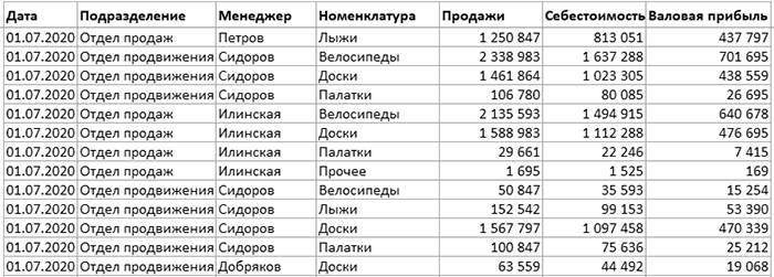
Что такое сводная таблица Excel
Что такое сводная таблица (Pivot Table – англ.)? Pivot Table дословно переводится как «таблица, которую можно крутить, показывать в разных разворотах». Это инструмент, который позволяет представлять данные в виде, удобном для анализа. Вид сводной таблицы можно быстро менять с помощью одной только мышки, помещая данные в строки или столбцы, выбирать уровни группировки, фильтровать и «перетаскивать» мышкой столбцы с одного места на другое.
Также к сводным таблицам можно применять элементы управления и добавлять диаграммы, создавая наглядные отчеты. Примеры таких отчетов можно посмотреть здесь:
- Отчет о динамике и структуре продаж
- Анализ исполнения бюджета (БДР)
Исходные данные для сводной таблицы
Чтобы построить сводную таблицу, нужно обратиться к данным в Excel, организованным в виде плоской таблицы. Это значит, что все строки такой таблицы заполнены и в ней нет группировок.
Как построить сводную таблицу
Шаг 1. Выделить таблицу Excel
Выделите одну ячейку таблицы (тогда Excel автоматически определит границы таблицы на следующем шаге) или выделите всю таблицу вместе с заголовками.
Как быстро выделить таблицу:
- Выбрать ее любую ячейку и нажать Crtl + * или Ctrl + A, или
- Выбрать самую первую ячейку в таблице, зажать кнопки Ctrl и Shift, а затем нажать на кнопки вправо, затем вниз (→↓).
Если выделить больше одной ячейки, но не всю таблицу, в качестве источника данных будет захвачена только выделенная область.
Шаг 2. Создать сводную таблицу
Создайте сводную таблицу: перейдите на вкладку Вставка и выберите «Сводная таблица».
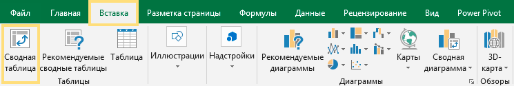
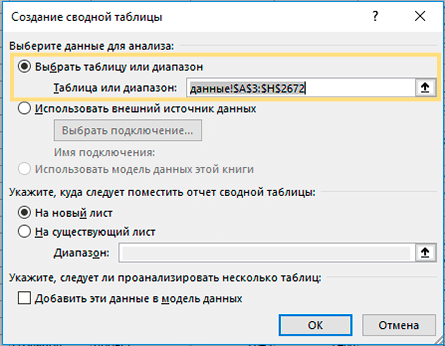
В появившемся диалоговом окне укажите исходные данные (если вы уже выделили таблицу, источник данных заполнится автоматически) и желаемое место расположения сводной таблицы. Её можно поместить на новый или существующий лист.
Когда сводная таблица добавлена, на листе появляется область сводной таблицы. Если эта область не активна (вы не выделили ее мышкой), на ней будет подсказка: «Чтобы начать работу с отчетом сводной таблицей, щелкните в этой области». Щелкаем по ней мышкой и происходят две вещи:
- Справа появится список полей сводной таблицы.
- В меню — две дополнительные вкладки, связанные с управлением сводной таблицей (Анализ и Конструктор).
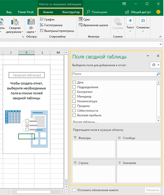
Шаг 3. Добавить в сводную таблицу необходимые поля
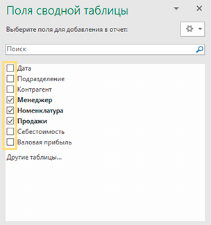 Проставляем «галочки» в нужных полях сводной таблицы. При этом элементы «сами» встанут на свои места. Если просто поставить «галочки» в области выбора полей, Excel в зависимости от содержимого ячеек определит куда что ставить. Если в столбце содержатся только значения в числовом формате, то его содержимое попадет в область «Σ Значения».
Правило следующее: если поле содержит текст или числа хотя бы с одной пустой или текстовой ячейкой, то Excel автоматически поместит эти данные в область «Названия строк».
После заполнения областей сводной таблицы её вид изменится. В нашем примере в строках появились ФИО менеджеров и товары, а напротив них – суммы продаж. Далее данные можно детализировать и создать визуализации.
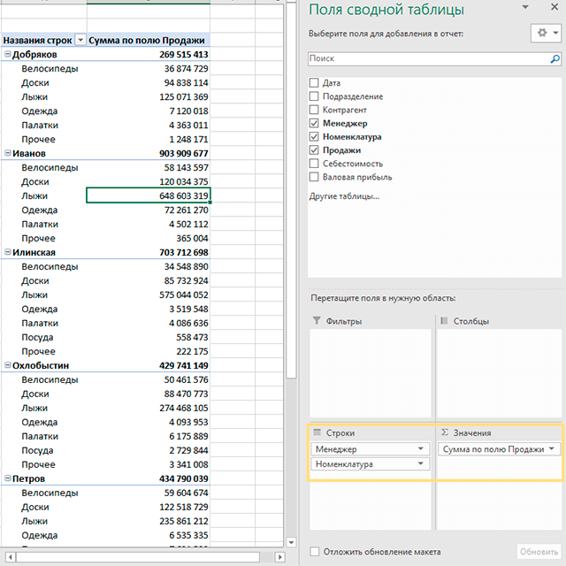
Поля можно «перетаскивать» мышкой из одной области в другую:

- Фильтры. С помощью фильтров отбираем из исходных данных нужную информацию. Для этого поместите поля в область фильтров и выберите значения, которые хотите анализировать.
- Столбцы – поместите в эту область поля, которые должны быть в заголовках столбцов.
- Строки – данные, которые будут выводиться в строках таблицы.
В область строк и столбцов можно поместить несколько полей. Тогда данные в таблице будут сгруппированы. - Область значений. В этой области размещаем числовые показатели, которые нужно просуммировать или рассчитать среднее, минимум, максимум и т.д.
Обновление сводной таблицы
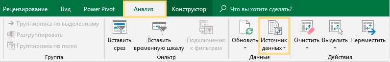
Когда исходные данные поменяются, обновите сводную таблицу. Для этого перейдите в меню Данные и нажмите «Обновить». Такая же кнопка есть и на вкладке Анализ. Или еще можно щелкнуть правой кнопкой мышки по сводной таблице и выбрать «Обновить» в появившемся меню. После нажатия этой кнопки сводная таблица «пересчитается».
Если изменился сам источник данных (добавлены новые строки или столбцы), выберите любую ячейку сводной таблицы и перейдите в меню Анализ → Источник данных.
В появившемся окне выберите источник данных.
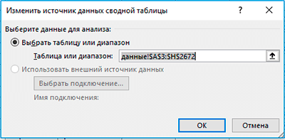
Один из оптимальных способов задать источник данных – это указать в качестве него «умную» smart-таблицу Excel. О преимуществах этого способа и вообще о плюсах использования «умных» таблиц читайте в следующей статье.
Резюме
В этой статье рассмотрен пример создания простой сводной таблицы, с помощью которой данные можно группировать, анализировать и представлять в нужном нам виде за несколько щелчков мышки. Так что сводные таблицы – это полезный инструмент, который пригодится вам в будущем.
То, что написано о сводных таблицах в статье — это еще не все. Для «продвинутой» аналитики в Excel есть надстройки и инструменты, которые расширяют функционал сводных таблиц до действительно серьезного уровня и переносят его в область Business Intelligence. Сейчас мы говорим о надстройках Power Query и Power Pivot, которые также задействованы в продукте Microsoft Power BI.
Pivot tables are a well-known, often misunderstood feature of Excel. They have a reputation for being one of the more advanced features of the software, but in fact, making pivot tables is quite straightforward.
Pivot tables make your data more intuitive and straightforward. This is great if you deal with large amounts of data and want to organize it in a more readable way or if you need to analyze data that others can easily interpret at a glance.
In this article, you’ll learn how to make a pivot table in Excel and how and when to use a pivot table. We’ll also show you how to effectively customize your pivot tables so that you receive the exact results you need, and also how to update your pivot table after any changes to your original dataset.
What is a pivot table?
Pivot tables summarize your data in a chart that lets you interpret what the data actually means. They essentially reorganize your data by pivoting the columns into rows and rows into columns, so that you can see your data in a different way.
What can I use a pivot table for?
There are many ways you can use a pivot table. In general, pivot tables are used to effectively summarize, calculate and analyze large amounts of data in a format that lets you easily identify key patterns, trends, and comparisons.
- Summarize data in a more user-friendly way for others to see.
- Compare multiple rows and columns of data for report analytics.
- Group and sort data to find trends in numbers.
- Apply advanced calculations to your data easily.
For a more in-depth example, let’s say you have a dataset containing the total sales of each team member across multiple departments of your department store. Rather than manually adding up the total sales for each department, you can use a pivot table to automatically organize, combine and total the data for you. Not only does it save you time, but it also presents the data in a more readable way, so you can easily see everything you need at a glance.
How to create a pivot table in Excel step-by-step?
Creating a pivot table in Excel is more simple than you think. So what is the first step for creating a pivot table? Here’s a step-by-step of everything you need to do to create a pivot table in Excel from start to finish, using the example mentioned above as context.
Create data for a pivot table
- 1. Add your data directly into your workbook, or import data from an external source by selecting Data > Get data and select data from your desired source file.
Here is an example of my data of team members’ total sales across each department.

How to Create a Pivot Table in Excel — Create data for pivot table
- 2. Highlight all of your data and click “Format as Table” located in the toolbar. Make sure your entire table range is selected. Choose your preferred table style.

How to Create a Pivot Table in Excel — Format as Table
Your data should look something like this:

How to Create a Pivot Table in Excel — Excel data format table
Sort your data
It’s important that you sort your data according to your needs before turning it into a pivot table. This makes it a lot easier to manage as a final product.
- 1. Click the “Data” tab and select “Sort”. You can choose which column you want to sort by, the contents to sort by, and the order to sort by. Once you’re done, press “Ok”.

How to Create a Pivot Table in Excel — Sort data excel table
Now that your data is successfully formatted and sorted, it’s time to create your pivot table.
Create a pivot table
- 1. Click on one of the cells in your table and head to Insert > Pivot Table.

- 2. Excel should automatically select your entire table, but make sure all of your cells are included in the range. You can also choose where the pivot table will be located. Once you’re happy with everything, click “Ok”.

How to Create a Pivot Table in Excel — Create pivot table
Build a pivot table
It’s simple to build your pivot table to present your data as you want it.
- 1. Add data fields to your pivot table “Row labels” box. These will appear as the different rows in the pivot table.
For example, in order to get the total sales for each department, I can simply tick the “Department” and “Total sales” fields.

How to Create a Pivot Table in Excel — Add pivot table fields
- 2. Drag the fields to the “Filters”, “Columns”, “Rows” and “Values” boxes to customize your pivot table. Here’s what each box means:
- Filters: Add a filter for your data. For example, if I drag “Department” to the “Filter” box, I can receive the total number of sales for a custom selection of departments.

How to Create a Pivot Table in Excel — Add filters to pivot table
- Columns: Add a field as a column in your pivot table. For example, if I drag “Name” to the “Column” box, I can easily see the sales of each team member and which department they are in.

How to Create a Pivot Table in Excel — Add columns to pivot table
- Rows: Add a field as rows in your pivot table. For example, if I drag “Name” to the “Row” box, I can easily see which team member is in which department, and how much they sold.

How to Create a Pivot Table in Excel — Add rows to pivot table
- Values: Add new calculations to your pivot table. For example, if I drag “Total sales” to the “Values” box, I receive the total sales for each department, and the total sales combined.

How to Create a Pivot Table in Excel — Add values to pivot table
How to VLOOKUP in Excel with Two Spreadsheets?
Sometimes our data may be spread out among different Excel sheets or workbooks. Here’s how to do VLOOKUP in Excel with two spreadsheets
READ MORE

Customize your pivot table
With the foundations of your pivot table built, you can customize it further to receive specific insights. To do this, all you have to do is click on the “information” icon next to each field in the boxes to alter the type of data you receive.
- 1. Click the “information” icon next to one of your fields in a box. Adjust the settings based on the type of results you wish to receive.
In this example, I’ll select the “Total sales” field in the “Values” box and adjust the settings. As a result, I can now see the percentage that each department makes up for the total combined sales.

How to Create a Pivot Table in Excel — Customize pivot table
Update your pivot table
Let’s say you want to update your pivot table to reflect the new changes to your original table of data.
- 1. Add the changes to your original table of data. Make sure that the table format is applied to all of your cells.
In this example, I want to add a new sales member to the table. I’ve added their name, department, and total sales values to the worksheet, and made sure that the table formatting is applied to their row.

How to Create a Pivot Table in Excel — Add new data pivot table
- 2. Head back to the pivot table, right-click on a cell, and press “Refresh”.

How to Create a Pivot Table in Excel — Refresh pivot table
As you can see, the pivot table now includes my new row of data.

How to Create a Pivot Table in Excel — Update pivot table
Create a pivot table from multiple worksheets or workbooks
Creating a pivot table is simpler when your data is consolidated in one worksheet. However, if that isn’t possible, you should consolidate your data from multiple worksheets or workbooks into one master worksheet, using the “PivotTable and PivotChart Wizard”. Once you’ve done this, simply follow the same steps listed above. Read the Microsoft support page for more details on how to do this.
Want to Boost Your Team’s Productivity and Efficiency?
Transform the way your team collaborates with Confluence, a remote-friendly workspace designed to bring knowledge and collaboration together. Say goodbye to scattered information and disjointed communication, and embrace a platform that empowers your team to accomplish more, together.
Key Features and Benefits:
- Centralized Knowledge: Access your team’s collective wisdom with ease.
- Collaborative Workspace: Foster engagement with flexible project tools.
- Seamless Communication: Connect your entire organization effortlessly.
- Preserve Ideas: Capture insights without losing them in chats or notifications.
- Comprehensive Platform: Manage all content in one organized location.
- Open Teamwork: Empower employees to contribute, share, and grow.
- Superior Integrations: Sync with tools like Slack, Jira, Trello, and more.
Limited-Time Offer: Sign up for Confluence today and claim your forever-free plan, revolutionizing your team’s collaboration experience.
Conclusion
Despite their intimidating reputation, pivot tables are easy to create and use. They offer a range of impressive insights that can be applied to almost any circumstance, whether you’re looking to summarize your data for financial reports or find the latest trends in blog post views.
By the end of this article, you should now know exactly what pivot tables can do, how to create one from your workbook, and how to customize and update them to suit your needs.