
Excel for Microsoft 365 Excel 2021 Excel 2019 Excel 2016 Excel 2013 Excel 2010 More…Less
Excel is an incredibly powerful tool for getting meaning out of vast amounts of data. But it also works really well for simple calculations and tracking almost any kind of information. The key for unlocking all that potential is the grid of cells. Cells can contain numbers, text, or formulas. You put data in your cells and group them in rows and columns. That allows you to add up your data, sort and filter it, put it in tables, and build great-looking charts. Let’s go through the basic steps to get you started.
Excel documents are called workbooks. Each workbook has sheets, typically called spreadsheets. You can add as many sheets as you want to a workbook, or you can create new workbooks to keep your data separate.
-
Click File, and then click New.
-
Under New, click the Blank workbook.

-
Click an empty cell.
For example, cell A1 on a new sheet. Cells are referenced by their location in the row and column on the sheet, so cell A1 is in the first row of column A.
-
Type text or a number in the cell.
-
Press Enter or Tab to move to the next cell.
-
Select the cell or range of cells that you want to add a border to.
-
On the Home tab, in the Font group, click the arrow next to Borders, and then click the border style that you want.
For more information, see Apply or remove cell borders on a worksheet .
-
Select the cell or range of cells that you want to apply cell shading to.
-
On the Home tab, in the Font group, choose the arrow next to Fill Color
, and then under Theme Colors or Standard Colors, select the color that you want.
 , and then under Theme Colors or Standard Colors, select the color that you want.
For more information about how to apply formatting to a worksheet, see Format a worksheet.
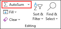
When you’ve entered numbers in your sheet, you might want to add them up. A fast way to do that is by using AutoSum.
-
Select the cell to the right or below the numbers you want to add.
-
Click the Home tab, and then click AutoSum in the Editing group.
AutoSum adds up the numbers and shows the result in the cell you selected.
For more information, see Use AutoSum to sum numbers
Adding numbers is just one of the things you can do, but Excel can do other math as well. Try some simple formulas to add, subtract, multiply, or divide your numbers.
-
Pick a cell, and then type an equal sign (=).
That tells Excel that this cell will contain a formula.
-
Type a combination of numbers and calculation operators, like the plus sign (+) for addition, the minus sign (-) for subtraction, the asterisk (*) for multiplication, or the forward slash (/) for division.
For example, enter =2+4, =4-2, =2*4, or =4/2.
-
Press Enter.
This runs the calculation.
You can also press Ctrl+Enter if you want the cursor to stay on the active cell.
For more information, see Create a simple formula.
To distinguish between different types of numbers, add a format, like currency, percentages, or dates.
-
Select the cells that have numbers you want to format.
-
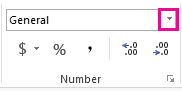
Click the Home tab, and then click the arrow in the General box.
-
Pick a number format.
If you don’t see the number format you’re looking for, click More Number Formats. For more information, see Available number formats.

A simple way to access Excel’s power is to put your data in a table. That lets you quickly filter or sort your data.
-
Select your data by clicking the first cell and dragging to the last cell in your data.
To use the keyboard, hold down Shift while you press the arrow keys to select your data.
-
Click the Quick Analysis button
in the bottom-right corner of the selection.
-
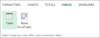
Click Tables, move your cursor to the Table button to preview your data, and then click the Table button.
-
Click the arrow
in the table header of a column. -
To filter the data, clear the Select All check box, and then select the data you want to show in your table.
-
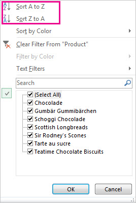
To sort the data, click Sort A to Z or Sort Z to A.
-
Click OK.
 in the bottom-right corner of the selection.
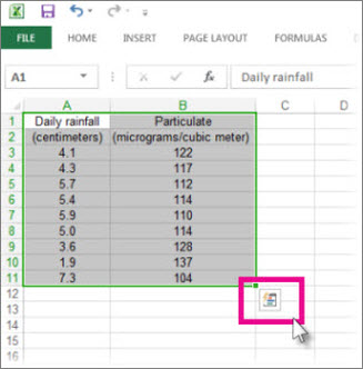
 in the table header of a column.
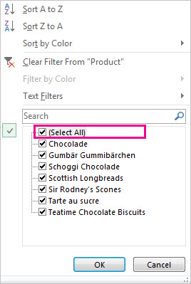
For more information, see Create or delete an Excel table
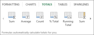
The Quick Analysis tool (available in Excel 2016 and Excel 2013 only) let you total your numbers quickly. Whether it’s a sum, average, or count you want, Excel shows the calculation results right below or next to your numbers.
-
Select the cells that contain numbers you want to add or count.
-
Click the Quick Analysis button
in the bottom-right corner of the selection. -
Click Totals, move your cursor across the buttons to see the calculation results for your data, and then click the button to apply the totals.
Conditional formatting or sparklines can highlight your most important data or show data trends. Use the Quick Analysis tool (available in Excel 2016 and Excel 2013 only) for a Live Preview to try it out.
-
Select the data you want to examine more closely.
-
Click the Quick Analysis button
in the bottom-right corner of the selection. -
Explore the options on the Formatting and Sparklines tabs to see how they affect your data.
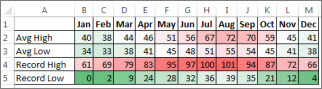
For example, pick a color scale in the Formatting gallery to differentiate high, medium, and low temperatures.
-
When you like what you see, click that option.
 in the bottom-right corner of the selection.
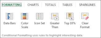
Learn more about how to analyze trends in data using sparklines.
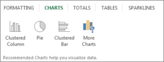
The Quick Analysis tool (available in Excel 2016 and Excel 2013 only) recommends the right chart for your data and gives you a visual presentation in just a few clicks.
-
Select the cells that contain the data you want to show in a chart.
-
Click the Quick Analysis button
in the bottom-right corner of the selection. -
Click the Charts tab, move across the recommended charts to see which one looks best for your data, and then click the one that you want.
Note: Excel shows different charts in this gallery, depending on what’s recommended for your data.
Learn about other ways to create a chart.
To quickly sort your data
-
Select a range of data, such as A1:L5 (multiple rows and columns) or C1:C80 (a single column). The range can include titles that you created to identify columns or rows.
-
Select a single cell in the column on which you want to sort.
-
Click
to perform an ascending sort (A to Z or smallest number to largest). -
Click
to perform a descending sort (Z to A or largest number to smallest).
 to perform an ascending sort (A to Z or smallest number to largest).
 to perform a descending sort (Z to A or largest number to smallest).
To sort by specific criteria
-
Select a single cell anywhere in the range that you want to sort.
-
On the Data tab, in the Sort & Filter group, choose Sort.
-
The Sort dialog box appears.
-
In the Sort by list, select the first column on which you want to sort.
-
In the Sort On list, select either Values, Cell Color, Font Color, or Cell Icon.
-
In the Order list, select the order that you want to apply to the sort operation — alphabetically or numerically ascending or descending (that is, A to Z or Z to A for text or lower to higher or higher to lower for numbers).
For more information about how to sort data, see Sort data in a range or table .
-
Select the data that you want to filter.
-
On the Data tab, in the Sort & Filter group, click Filter.
-
Click the arrow
in the column header to display a list in which you can make filter choices. -
To select by values, in the list, clear the (Select All) check box. This removes the check marks from all the check boxes. Then, select only the values you want to see, and click OK to see the results.
For more information about how to filter data, see Filter data in a range or table.
-
Click the Save button on the Quick Access Toolbar, or press Ctrl+S.
If you’ve saved your work before, you’re done.
-
If this is the first time you’ve save this file:
-
Under Save As, pick where to save your workbook, and then browse to a folder.
-
In the File name box, enter a name for your workbook.
-
Click Save.
-

-
Click File, and then click Print, or press Ctrl+P.
-
Preview the pages by clicking the Next Page and Previous Page arrows.
The preview window displays the pages in black and white or in color, depending on your printer settings.
If you don’t like how your pages will be printed, you can change page margins or add page breaks.
-
Click Print.

-
On the File tab, choose Options, and then choose the Add-Ins category.
-
Near the bottom of the Excel Options dialog box, make sure that Excel Add-ins is selected in the Manage box, and then click Go.
-
In the Add-Ins dialog box, select the check boxes the add-ins that you want to use, and then click OK.
If Excel displays a message that states it can’t run this add-in and prompts you to install it, click Yes to install the add-ins.
For more information about how to use add-ins, see Add or remove add-ins.
Excel allows you to apply built-in templates, to apply your own custom templates, and to search from a variety of templates on Office.com. Office.com provides a wide selection of popular Excel templates, including budgets.
For more information about how to find and apply templates, see Download free, pre-built templates.
Need more help?
Want more options?
Explore subscription benefits, browse training courses, learn how to secure your device, and more.
Communities help you ask and answer questions, give feedback, and hear from experts with rich knowledge.
How To Use Excel:
A Beginner’s Guide To Getting Started
Written by co-founder Kasper Langmann, Microsoft Office Specialist.
Excel is a powerful application—but it can also be very intimidating.
That’s why we’ve put together this beginner’s guide to getting started with Excel.
It will take you from the very beginning (opening a spreadsheet), through entering and working with data, and finish with saving and sharing.
It’s everything you need to know to get started with Excel.
If you want to tag along as you read, please download the free sample Excel workbook here.
Opening an Excel spreadsheet
When you first open Excel (by double-clicking the icon or selecting it from the Start menu), the application will ask what you want to do.

If you want to open a new Excel spreadsheet, click Blank workbook.
To open an existing spreadsheet (like the example workbook you just downloaded), click Open Other Workbooks in the lower-left corner, then click Browse on the left side of the resulting window.

Then use the file explorer to find the Excel workbook you’re looking for, select it, and click Open.
Workbooks vs. spreadsheets
There’s something we should clear up before we move on.
A workbook is an Excel file. It usually has a file extension of .XLSX (if you’re using an older version of Excel, it could be .XLS).
A spreadsheet is a single sheet inside a workbook. There can be many sheets inside of a workbook, and they’re accessed via the tabs at the bottom of the screen.
A spreadsheet (a.k.a. a sheet/tab) contains all the cells you can see and use in the >1 million rows >16,000 columns.
Working with the Ribbon
The Ribbon is the central control panel of Excel. You can do just about everything you need to directly from the Ribbon.
Where is this powerful tool? At the top of the window:

There are a number of tabs, including the File tab, Home tab, Insert tab, Data tab, Review tab, and a few others. Each tab contains different buttons.
Try clicking on a few different tabs to see which buttons appear below them.
 Kasper Langmann, Co-founder of Spreadsheeto
There’s also a very useful search bar in the Ribbon. It says Tell me what you want to do. Just type in what you’re looking for, and Excel will help you find it.

Most of the time, you’ll be in the Home tab of the Ribbon. But Formulas and Data are also very useful (we’ll be talking about formulas shortly).
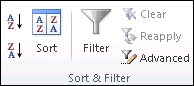
Pro tip: Ribbon sections
In addition to tabs, the Ribbon also has some smaller sections. And when you’re looking for something specific, those sections can help you find it.
For example, if you’re looking for sorting and filtering options, you don’t want to hover over dozens of buttons finding out what they do.
Instead, skim through the section names until you find what you’re looking for:

Managing your sheets
As we saw, workbooks can contain multiple sheets.
You can manage those sheets with the sheet tabs near the bottom of the screen. Click a tab to open that particular worksheet.
If you’re using our example workbook, you’ll see two sheets, called Welcome and Thank You:

To add a new worksheet, click the + (plus) button at the end of the list of sheets.
You can also reorder the sheets in your workbook by dragging them to a new location.
And if you right-click a worksheet tab, you’ll get a number of options:

For now, don’t worry too much about these options. Rename and Delete are useful, but the rest needn’t concern you.
Kasper Langmann, Co-founder of SpreadsheetoEntering data
Now it’s time to enter some data!
And while entering data is one of the most central and important things you can do in Excel, it’s almost effortless.
Just click into a blank cell and start typing.
Go ahead, try it! Type your name, birthday, and your favorite number into some blank cells.
Kasper Langmann, Co-founder of SpreadsheetoYou can also copy (Ctrl + C), cut (Ctrl + X), and paste (Ctrl + V) any data you’d like (or read our full guide on copying and pasting here).
Try copying and pasting the data from multiple cells inthe example spreadsheet into another column.
You can also copy data from other programs into Excel.
Try copying this list of numbers and pasting it into your sheet:
- 17
- 24
- 9
- 00
- 3
- 12
That’s all we’re going to cover for basic data entry. Just know that there are lots of other ways to get data into your spreadsheets if you need them.
Kasper Langmann, Co-founder of SpreadsheetoBasic calculations
Now that we’ve seen how to get some basic data into our spreadsheet, we’re going to do some things with it.
Running basic calculations in Excel is easy. First, we’ll look at how to add two numbers.
Important: start calculations with = (equals)
When you’re running a calculation (or a formula, which we’ll discuss next), the first thing you need to type is an equals sign. This tells Excel to get ready to run some sort of calculation.
So when you see something like =MEDIAN(A2:A51), make sure you type it exactly as it is—including the equals sign.
Let’s add 3 and 4. Type the following formula in a blank cell:
=3+4
Then hit Enter.

When you hit Enter, Excel evaluates your equation and displays the result, 7.
But if you look above at the formula bar, you’ll still see the original formula.
That’s a useful thing to keep in mind, in case you forget what you typed originally.
You can also edit a cell in the formula bar. Click on any cell, then click into the formula bar and start typing.
Kasper Langmann, Co-founder of SpreadsheetoPerforming subtraction, multiplication, and division is just as easy. Try these formulas:
- =4-6
- =2*5
- =-10/3
What we’re going to cover next is one of the most important things in Excel. We’re giving it a very basic overview here, but feel free to read our post on cell references to get the details.
Kasper Langmann, Co-founder of SpreadsheetoNow let’s try something different. Open up the first sheet in the example workbook, click into cell C1, and type the following:
=A1+B1
Hit Enter.
You should get 82, the sum of the numbers in cells A1 and B1.
Now, change one of the numbers in A1 or B1 and watch what happens:
Because you’re adding A1 and B1, Excel automatically updates the total when you change the values in one of those cells.
Try doing different types of arithmetic on the other numbers in columns A and B using this method.
Unlocking the power of functions
Excel’s greatest power lies in functions. These let you run complex calculations with a few keypresses.
We’ll barely scratch the surface of functions here. Check out our other blog posts to see some of the great things you can do with functions!
Kasper Langmann, Co-founder of SpreadsheetoMany formulas take sets of numbers and give you information about them.
For example, the AVERAGE function gives you the average of a set of numbers. Let’s try using it.
Click into an empty cell and type the following formula:
=AVERAGE(A1:A4)
Then hit Enter.

The resulting number, 0.25, is the average of the numbers in cells A1, A2, A3, and A4.
Cell range notation
In the formula above, we used “A1:A4” to tell Excel to look at all the cells between A1 and A4, including both of those cells. You can read it as “A1 through A4.”
You can also use this to include numbers in different columns. “A5:C7” includes A5, A6, A7, B5, B6, B7, C5, C6, and C7.
There are also functions that work on text.
Let’s try the CONCATENATE function!
Click into cell C5 and type this formula:
=CONCATENATE(A5, ” “, B5)
Then hit Enter.
You’ll see the message “Welcome to Spreadsheeto” in the cell.
How did this happen? CONCATENATE takes cells with text in them and puts them together.
We put the contents of A5 and B5 together. But because we also needed a space between “to” and “Spreadsheeto,” we included a third argument: the space between two quotes.
Remember that you can mix cell references (like “A5″) and typed values (like ” “) in formulas.
Kasper Langmann, Co-founder of SpreadsheetoExcel has dozens of useful functions. To find the function that will solve a particular problem, head to the Formulas tab and click on one of the icons:

Scroll through the list of available functions, and select the one you want (you may have to look around for a while).
Then Excel will help you get the right numbers in the right places:

If you start typing a formula, starting with the equals sign, Excel will help you by showing you some possible functions that you might be looking for:

And finally, once you’ve typed the name of a formula and the opening parenthesis, Excel will tell you which arguments need to go where:

If you’ve never used a function before, it might be difficult to interpret Excel’s reminders. But once you get more experience, it’ll become clear.
This is a tiny preview of how functions work and what they can do. It should be enough to get you going on the tasks you need to accomplish right away.
Kasper Langmann, Co-founder of SpreadsheetoSaving and sharing your work
After you’ve done a bunch of work with your spreadsheet, you’re going to want to save your changes.
Hit Ctrl + S to save. If you haven’t yet saved your spreadsheet, you’ll be asked where you want to save it and what you want to call it.
You can also click the Save button in the Quick Access Toolbar:

It’s a good idea to get into the habit of saving often. Trying to recover unsaved changes is a pain!
Kasper Langmann, Co-founder of SpreadsheetoThe easiest way to share your spreadsheets is via OneDrive.
Click the Share button in the top-right corner of the window, and Excel will walk you through sharing your document.

You can also save your document and email it, or use any other cloud service to share it with others.
That’s it – Now what?
This was how to use Excel.
Or… at least a small fraction of it.
Microsoft Excel can be intimidating, but once you get the basics down, it’s easier to learn the more advanced functions.
This was your introduction to “the basics”. So, if you’re not ready to get some advanced Excel knowledge, go ahead and practice with some of the existing data at the office 🧑🏼💻
If you’re ready to take your next steps, go ahead and enroll in my 30-minute free online course where you learn: IF, SUMIF, VLOOKUP, and data cleaning.
These are some of the most important topics of Excel💪🏼
Other resources
Now, you can’t excel at Excel without mastering some of the lookup functions like VLOOKUP and the new XLOOKUP.
But also, you don’t wanna miss out on pivot tables. You can use these to transform your Microsoft Excel data into insightful reports in just a few clicks🤯
Or if you’re into automating Excel spreadsheet formatting, go ahead and read my guide to conditional formatting here.
Kasper Langmann2023-02-23T14:45:07+00:00
Page load link
So, you have decided that time has come to become an Excel Master. Congratulations!
Before you start with Excel functions and tools, there are some basics that need to be covered first.
Let’s start our magical journey in Excel together! 🙂
A really quick intro to Excel
Excel is the world’s most popular spreadsheet software, developed by Microsoft.
Excel debuted on September 30, 1985, and since that day, kept evolving to meet the requirements of the spreadsheet community.
Most of the Excel versions require installation on your local computer. However, In recent years, Excel can be used online, via Excel Online!
And the best thing? Excel Online is absolutely free.
This website utilizes the technology of Excel Online to help you learn and practice Excel without the need have Excel installed on your computer. Thanks Microsoft! 🙂
So, let’s finish with the talking and start practicing!
Typing in Excel
Excel can be used for complex calculations, but you can always use it to type regular text, just like you’d do in Word or any other software.
All you have to do is select one of the cells and start typing…
You can start by typing your name, your favorite pet, your favorite movie and your lucky number 🙂
When you finish typing, hit the Enter key to exit the cell edit mode.
As you can see, you can type both text and numbers in Excel.
Did you notice that certain parts of the sheets changed after you typed your details? This was done using Excel formulas, which we will cover in the next tutorials 🙂
How does Excel work?
Let’s discuss some of the basic ideas in Excel:
- Excel Cell
- Excel Range
- Excel Worksheet
- Excel Workbook
1. Excel Cell
The Excel Cell is the smallest unit in Excel. The cell is used to store data.
In the previous example, we typed our names and favorite pets, movies and numbers in different Excel Cells.
Excel is comprised of rows and columns. The rows are represented as numbers, and the columns – as letters.
In order to reference a specific cell in Excel, we will type its column letter, followed by the row number.
So, A1 will be the first cell in your worksheet – It’s in the first column (A), and in the first row (1):

Ok, now let’s practice… Type your First Name in cell C3, and your Last Name in cell C4
2. Excel Range
The Excel Range is comprised of two or more adjacent cells. These cells can be in the same row, the same column, or even in multiple rows and columns!
Each range is represented by two cells – The top-left cell, and the bottom-right cell, separated with colons.
For example, Range A3:E7 consists of the following cells:

Now, it’s your time to play with Excel ranges!
3. Excel Worksheet
The Excel Worksheet is comprised of rows and columns.
The default Excel Worksheet contains 1,048,576 rows and 16,384 columns.
In the following example, we have 4 different worksheets:

Tip – We can quickly navigate between worksheets using the shortcut Ctrl+Page Up/Ctrl+Page Down. Click here for more useful Excel shortcuts!
4. Excel Workbook
The Excel file is also called Excel Workbook. It contains one or more worksheets.
The default Excel file type has an XLSX suffix.
Excel allows the user to use data from one worksheet in another worksheet in the same workbook. It also allows connecting between different workbooks.
Basic Calculations with Excel
OK, let’s start with the fun part!
We can perform calculations in Excel easily.
In order to start a calculation in a cell, we will type the = sign (equals), and then type our calculation.
These are the basic operators which can be used:
+ Add
– Substract
/ Divide
* (Asterisk) Multiply
^ Power
So, let’s say we want to find the result of 2+2:

Ok, now let’s practice!
Cell References
Okay, now that we know how to perform basic calculations, let’s learn how we can use cell references to make our calculations much quicker, and dynamic, as well!
If we type the = (equals) sign, followed by a reference to a cell (either by typing the cell name or clicking it), we can reference the data stored in that cell. We can also perform calculations using this way – Instead of manually typing the numbers, we can just reference the cells containing these numbers!
Let’s see how it works:

You can see in the example above that each time we change the data in the referenced cell – It is automatically reflected in the second cell!
Now, time to play with Excel:
Reusing cell references & using Partial and Absolute References
One of the advantages of using cell references in Excel is that we can reuse cell references in adjacent cells by copying the cell, or by dragging the cell to adjacent cells.
Let’s see how it works:

Sometimes, we would like that a certain reference will not move if we reuse the formula in other cells.
In such cases, we can use an Absolute Reference, by hitting the F4 button (or manually typing the $ signs before the column and/or row – not recommended) after typing the cell reference.
Let’s see this in action:

In certain cases, we might prefer using a Partial Reference rather than an Absolute Reference.
A Partial Reference allows us to keep the same reference only for a part of the cell – either the row or the column.
To use Partial Reference, just hit the F4 button until the deserved result is achieved.
Let’s see how we can do the entire Multiplication Table calculation, using only one formula!

Now you are all set to continue your Excel journey and learn how to use Excel functions and tools. Good luck! 🙂
Excel is an electronic spreadsheet program that is used for storing, organizing and manipulating data. Data is stored in individual cells that are usually organized in a series of columns and rows in a worksheet; this collection of columns and rows is referred to as a table.
Spreadsheets programs can also perform calculations on the data using formulas. To help make it easier to find and read the information in a worksheet, Excel has a number of formatting features that can be applied to individual cells, rows, columns, and entire tables of data.
Since each worksheet in recent versions of Excel contains billions of cells per worksheet, each cell has an address known as a cell reference so that it can be referenced in formulas, charts, and other features of the program.
Topics included in this tutorial are:
- Entering the data into the table
- Widening individual worksheet columns
- Adding the current date and a named range to the worksheet
- Adding the deduction formula
- Adding the net salary formula
- Copying formulas with the Fill Handle
- Adding number formatting to data
- Adding cell formatting
Entering Data Into Your Worksheet
Entering the Tutorial Data.
Entering data into worksheet cells is always a three-step process; these steps are as follows:
- Click on the cell where you want the data to go.
- Type the data into the cell.
- Press the Enter key on the keyboard or click on another cell with the mouse.
As mentioned, each cell in a worksheet is identified by an address or cell reference, which consists of the column letter and number of the row that intersect at a cell’s location. When writing a cell reference, the column letter is always written first followed by the row number – such as A5, C3, or D9.
When entering the data for this tutorial, it is important to enter the data into the correct worksheet cells. Formulas entered in subsequent steps make use of the cell references of the data entered now.
To follow this tutorial, use the cell references of the data seen in the image above to enter all the data into a blank Excel worksheet.
Widening Columns in Excel
Widening Columns to Display the Data.
By default, the width of a cell permits only eight characters of any data entry to be displayed before that data spills over into the next cell to the right. If the cell or cells to the right are blank, the entered data is displayed in the worksheet, as seen with the worksheet title Deduction Calculations for Employees entered into cell A1.
If the cell to the right contains data, however, the contents of the first cell are truncated to the first eight characters. Several cells of data entered in the previous step, such as the label Deduction Rate: entered into cell B3 and Thompson A. entered into cell A8 are truncated because the cells to the right contain data.
To correct this problem so that the data is fully visible, the columns containing that data need to be widened. As with all Microsoft programs, there are multiple ways of widening columns. The steps below cover how to widen columns using the mouse.
Widening Individual Worksheet Columns
- Place the mouse pointer on the line between columns A and B in the column header.
- The pointer will change to a double-headed arrow.
- Click and hold down the left mouse button and drag the double-headed arrow to the right to widen column A until the entire entry Thompson A. is visible.
- Widen other columns to show data as needed.
Column Widths and Worksheet Titles
Since the worksheet title is so long compared to the other labels in column A, if that column was widened to display the entire title in cell A1, the worksheet would not only look odd, but it would make it difficult to use the worksheet because of the gaps between the labels on the left and the other columns of data.
As there are no other entries in row 1, it is not incorrect to just leave the title as it – spilling over into the cells to the right. Alternatively, Excel has a feature called merge and center which will be used in a later step to quickly center the title over the data table.
Adding the Date and a Named Range
Adding a Named Range to the Worksheet.
It is normal to add the date to a spreadsheet — quite often to indicate when the sheet was last updated. Excel has a number of date functions that make it easy to enter the date into a worksheet. Functions are just built-in formulas in Excel to make it easy to complete commonly performed tasks – such as adding the date to a worksheet.
The TODAY function is easy to use because it has no arguments – which is data that needs to be supplied to the function in order for it to work. The TODAY function is also one of Excel’s volatile functions, which means it updates itself every time the recalculates – which is usually ever time the worksheet is opened.
Adding the Date with the TODAY function
The steps below will add the TODAY function to cell C2 of the worksheet.
- Click on cell C2 to make it the active cell.
- Click on the Formulas tab of the ribbon.
- Click on the Date & Time option on the ribbon to open the list of date functions.
- Click on the Today function to bring up the Formula Builder.
- Click Done in the box to enter the function and return to the worksheet.
- The current date should be added to cell C2.
Seeing ###### Symbols instead of the Date
If a row of hashtag symbols appear in cell C2 instead of the date after adding the TODAY function to that cell, it is because the cell is not wide enough to display the formatted data.
As mentioned previously, unformatted numbers or text data spill over to empty cells to the right if it is too wide for the cell. Data that has been formatted as a specific type of number – such as currency, dates, or time, however, do not spill over to the next cell if they are wider than the cell where they are located. Instead, they display the ###### error.
To correct the problem, widen column C using the method described in the preceding step of the tutorial.
Adding a Named Range
A named range is created when one or more cells are given a name to make the range easier to identify. Named ranges can be used as a substitute for cell reference when used in functions, formulas, and charts. The easiest way to create named ranges is to use the name box located in the top left corner of the worksheet above the row numbers.
In this tutorial, the name rate will be given to cell C6 to identify the deduction rate applied to employee salaries. The named range will be used in the deduction formula that will be added to cells C6 to C9 of the worksheet.
- Select cell C6 in the worksheet.
- Type rate in the Name Box and press the Enter key on the keyboard
- Cell C6 now has the name of rate.
This name will be used to simplify creating the Deductions formulas in the next step of the tutorial.
Entering the Employee Deductions Formula
Entering the Deduction Formula.
Excel formulas allow you to perform calculations on number data entered into a worksheet. Excel formulas can be used for basic number crunching, such as addition or subtraction, as well as more complex calculations, such as finding a student’s average on test results and calculating mortgage payments.
- Formulas in Excel always begin with an equal sign ( = ).
- The equal sign is always typed into the cell where you want the answer to appear.
- The formula is completed by pressing the Enter key on the keyboard.
Using Cell References in Formulas
A common way of creating formulas in Excel involves entering the formula data into worksheet cells and then using the cell references for the data in the formula, instead of the data itself.
The main advantage of this approach is that if later it becomes necessary to change the data, it is a simple matter of replacing the data in the cells rather than rewriting the formula. The results of the formula will update automatically once the data changes.
Using Named Ranges in Formulas
An alternative to cell references is to used named ranges – such as the named range rate created in the previous step.
In a formula, a named range function the same as a cell reference but it is normally used for values that are used a number of times in different formulas – such as a deduction rate for pensions or health benefits, a tax rate, or a scientific constant – whereas cell references are more practical in formulas that refer to specific data only once.
Entering the Employee Deductions Formula
The first formula created in cell C6 will multiply the Gross Salary of the employee B. Smith by the deduction rate in cell C3.
The finished formula in cell C6 will be:
= B6 * rate
Using Pointing to Enter the Formula
Although it is possible to just type the above formula into cell C6 and have the correct answer appear, it is better to use pointing to add the cell references to formulas in order to minimize the possibility of errors created by typing in the wrong cell reference.
Pointing involves clicking on the cell containing the data with the mouse pointer to add the cell reference or named range to the formula.
- Click on cell C6 to make it the active cell.
- Type the equal sign ( = ) into cell C6 to begin the formula.
- Click on cell B6 with the mouse pointer to add that cell reference to the formula after the equal sign.
- Type the multiplication symbol (*) in cell C6 after the cell reference.
- Click on cell C3 with the mouse pointer to add the named range rate to the formula.
- Press the Enter key on the keyboard to complete the formula.
- The answer 2747.34 should be present in cell C6.
- Even though the answer to the formula is shown in cell C6, clicking on that cell will display the formula, = B6 * rate, in the formula bar above the worksheet
Entering the Net Salary Formula
Entering the Net Salary Formula.
This formula is created in cell D6 and calculates an employee’s net salary by subtracting the deduction amount calculated in the first formula from the Gross Salary. The finished formula in cell D6 will be:
= B6 - C6
- Click on cell D6 to make it the active cell.
- Type the equal sign ( = ) into cell D6.
- Click on cell B6 with the mouse pointer to add that cell reference to the formula after the equal sign.
- Type a minus sign( — ) in cell D6 after the cell reference.
- Click on cell C6 with the mouse pointer to that cell reference to the formula.
- Press the Enter key on the keyboard to complete the formula.
- The answer 43,041.66 should be present in cell D6.
Relative Cell References and Copying Formulas
So far, the Deductions and Net Salary formulas have been added to only one cell each in the worksheet – C6 and D6 respectively. As a result, the worksheet is currently complete for only one employee — B. Smith.
Rather than going through the time-consuming task of recreating each formula for the other employees, Excel permits, in certain circumstances, formulas to be copied to other cells. These circumstances most often involve the use of a specific type of cell reference – known as a relative cell reference – in the formulas.
The cell references that have been entered into the formulas in the preceding steps have been relative cell references, and they are the default type of cell reference in Excel, in order to make copying formulas as straightforward as possible.
The next step in the tutorial uses the Fill Handle to copy the two formulas to the rows below in order to complete the data table for all employees.
Copying Formulas with the Fill Handle
Using the Fill Handle to Copy Formulas.
The fill handle is a small black dot or square in the bottom right corner of the active cell. The fill handle has a number of uses including copying a cell’s contents to adjacent cells. filling cells with a series of numbers or text labels, and copying formulas.
In this step of the tutorial, the fill handle will be used to copy both the Deduction and Net Salary formulas from cells C6 and D6 down to cells C9 and D9.
Copying Formulas with the Fill Handle
- Highlight cells B6 and C6 in the worksheet.
- Place the mouse pointer over the black square in the bottom right corner of cell D6 – the pointer will change to a plus sign (+).
- Click and hold down the left mouse button and drag the fill handle down to cell C9.
- Release the mouse button – cells C7 to C9 should contain the results of the Deduction formula and cells D7 to D9 the Net Salary formula.
Applying Number Formatting in Excel
Adding Number Formatting to the Worksheet.
Number formatting refers to the addition of currency symbols, decimal markers, percent signs, and other symbols that help to identify the type of data present in a cell and to make it easier to read.
Adding the Percent Symbol
- Select cell C3 to highlight it.
- Click on the Home tab of the ribbon.
- Click on the General option to open the Number Format drop-down menu.
- In the menu, click on the Percentage option to change the format of value in cell C3 from 0.06 to 6%.
Adding the Currency Symbol
- Select cells D6 to D9 to highlight them.
- On the Home tab of the ribbon, click on the General option to open the Number Format drop-down menu.
- Click on the Currency in the menu to change the formatting of the values in cells D6 to D9 to currency with two decimal places.
Applying Cell Formatting in Excel
Applying Cell Formatting to the Data.
Cell formatting refers to formatting options – such as applying bold formatting to text or numbers, changing data alignment, adding borders to cells, or using the merge and center feature to change the appearance of the data in a cell.
In this tutorial, the above-mentioned cell formats will be applied to specific cells in the worksheet so that it will match the finished worksheet.
Adding Bold Formatting
- Select cell A1 to highlight it.
- Click on the Home tab of the ribbon.
- Click on the Bold formatting option as identified in the image above to bold the data in cell A1.
- Repeat the above sequence of steps to bold the data in cells A5 to D5.
Changing Data Alignment
This step will change the default left alignment of several cells to center alignment.
- Select cell C3 to highlight it.
- Click on the Home tab of the ribbon.
- Click on the Center alignment option as identified in the image above to center the data in cell C3.
- Repeat the above sequence of steps to center align the data in cells A5 to D5.
Merge and Center Cells
The Merge and Center option combines a number of selected into one cell and centers the data entry in the leftmost cell across the new merged cell. This step will merge and center the worksheet title — Deduction Calculations for Employees.
- Select cells A1 to D1 to highlight them.
- Click on the Home tab of the ribbon.
- Click on the Merge & Center option as identified in the image above to merge cells A1 to D1 and center the title across these cells.
Adding Bottom Borders to Cells
This step will add bottom borders to the cells containing data in rows 1, 5, and 9
- Select the merged cell A1 to D1 to highlight it.
- Click on the Home tab of the ribbon.
- Click on the down arrow next to the Border option as identified in the image above to open the borders drop-down menu.
- Click on the Bottom Border option in the menu to add a border to the bottom of the merged cell.
- Repeat the above sequence of steps to add a bottom border to cells A5 to D5 and to cells A9 to D9.
Thanks for letting us know!
Get the Latest Tech News Delivered Every Day
Subscribe
![]()
Download Article
![]()
Download Article
Are you new to Microsoft Excel and need to work on a spreadsheet? Excel is so overrun with useful and complicated features that it might seem impossible for a beginner to learn. But don’t worry—once you learn a few basic tricks, you’ll be entering, manipulating, calculating, and graphing data in no time! This wikiHow tutorial will introduce you to the most important features and functions you’ll need to know when starting out with Excel, from entering and sorting basic data to writing your first formulas.
Things You Should Know
- Use Quick Analysis in Excel to perform quick calculations and create helpful graphs without any prior Excel knowledge.
- Adding your data to a table makes it easy to sort and filter data by your preferred criteria.
- Even if you’re not a math person, you can use basic Excel math functions to add, subtract, find averages and more in seconds.
-
1
Create or open a workbook. When people refer to «Excel files,» they are referring to workbooks, which are files that contain one or more sheets of data on individual tabs. Each tab is called a worksheet or spreadsheet, both of which are used interchangeably. When you open Excel, you’ll be prompted to open or create a workbook.
- To start from scratch, click Blank workbook. Otherwise, you can open an existing workbook or create a new one from one of Excel’s helpful templates, such as those designed for budgeting.
-
2
Explore the worksheet. When you create a new blank workbook, you’ll have a single worksheet called Sheet1 (you’ll see that on the tab at the bottom) that contains a grid for your data. Worksheets are made of individual cells that are organized into columns and rows.
- Columns are vertical and labeled with letters, which appear above each column.
- Rows are horizontal and are labeled by numbers, which you’ll see running along the left side of the worksheet.
- Every cell has an address which contains its column letter and row number. For example, the top-left cell in your worksheet’s address is A1 because it’s in column A, row 1.
- A workbook can have multiple worksheets, all containing different sets of data. Each worksheet in your workbook has a name—you can rename a worksheet by right-clicking its tab and selecting Rename.
- To add another worksheet, just click the + next to the worksheet tab(s).
Advertisement
-
3
Save your workbook. Once you save your workbook once, Excel will automatically save any changes you make by default.[1]
This prevents you from accidentally losing data.- Click the File menu and select Save As.
- Choose a location to save the file, such as on your computer or in OneDrive.
- Type a name for your workbook. All workbooks will automatically inherit the the .XLSX file extension.
- Click Save.


Advertisement
-
1
Click a cell to select it. When you click a cell, it will highlight to indicate that it’s selected.
- When you type something into a cell, the input text is called a value. Entering data into Excel is as simple as typing values into each cell.
- When entering data, the first row of your worksheet (e.g., A1, B1, C1) is typically used as headers for each column. This is helpful when creating graphs or tables which require labels.
- For example, if you’re adding a list of dates in column A, you might click cell A1 and type Date into the cell as the column header.
-
2
Type a word or number into the cell. As you’re typing, you’ll see the letters and/or numbers appear in the cell, as well as in the formula bar at the top of the worksheet.
- When you start practicing more advanced Excel features like creating formulas, this bar will come in handy.
- You can also copy and paste text from other applications into your worksheet, tables from PDFs and the web.
-
3
Press ↵ Enter or ⏎ Return. This enters the data into the cell and moves to the next cell in the column.
-
4
Automatically fill columns based on existing data. Let’s say you want to make a list of consecutive dates or numbers. Or what if you want to fill a column with many of the same values that follow a pattern? As long as Excel can recognize some sort of pattern in your data, such as a particular order, you can use Autofill to automatically populate data into the rest of your column. Here’s a trick to see it in action.
- In a blank column, type 1 into the first cell, 2 into the second cell, and then 3 into the third cell.
- Hover your mouse cursor over the bottom-right corner of the last cell in your series—it will turn to a crosshair.
- Click and drag the crosshair down the column, then release the mouse button once you’ve gone down as far as you like. By default, this will fill the remaining cells with the value of the selected cell—at this point, you’ll probably have something like 1, 2, 3, 3, 3, 3, 3, 3.
- Click the small icon at the bottom-right corner of the filled data to open AutoFill options, and select Fill Series to automatically detect the series or pattern. Now you’ll have a list of consecutive numbers. Try this cool feature out with different patterns!
- Once you get the hang of AutoFill, you’ll have to try flash fill, which you can use to join two columns of data into a single merged column.
-
5
Adjust the column sizes so you can see all of the values. Sometimes typing long values into a cell hides the value and displays hash symbols ### instead of what you’ve typed. If you want to be able to see everything, you can snap the cell contents to the width of the widest cell. For example, let’s say we have some long values in column B:
- To expand the contents of column B, hover the cursor over the dividing line between the B and C at the top of the worksheet—once your cursor is right on the line, it will turn to two arrows pointing in either direction.[2]
- Click and drag the separator until the column is wide enough to accommodate your data, or just double-click the separator to instantly snap the column to the size of the widest value.
- To expand the contents of column B, hover the cursor over the dividing line between the B and C at the top of the worksheet—once your cursor is right on the line, it will turn to two arrows pointing in either direction.[2]
-
6
Wrap text in a cell. If your longer values are now awkwardly long, you can enable text wrapping in one or more cells. Just click a cell (or drag the mouse to select multiple cells), click the Home tab, and then click Wrap Text on the toolbar.
-
7
Edit a cell value. If you need to make a change to a cell, you can double-click the cell to activate the cursor, and then make any changes you need. When you’re finished, just press Enter or Return again.
- To delete the contents of a cell, click the cell once and press delete on your keyboard.
-
8
Apply styles to your data. Whether you want to highlight certain values with color so they stand out or just want to make your data look pretty, changing the colors of cells and their containing values is easy—especially if you’re used to Microsoft Word:
- Select a cell, column, row, or multiple cells at once.
- On the Home tab, click Cell Styles if you’d like to quickly apply quick color styles.
- If you’d rather use more custom options, right-click the selected cell(s) and select Format Cells. Then, use the colors on the Fill tab to customize the cell’s background, or the colors on the Font tab for value colors.
-
9
Apply number formatting to cells containing numbers. If you have data that contains numbers such as prices, measurements, dates, or times, you can apply number formatting to the data so it will display consistently.[3]
By default, the number format is General, which means numbers display exactly as you type them.- Select the cell you want to format. If you’re working with an entire column or row, you can just click the column letter or row number to select the whole thing.
- On the Home tab, click the drop-down menu at the top-center—it’ll say General by default, unless you selected cells that Excel recognizes as a different type of number like Currency or Time.
- Choose one of the formatting options in the list, such as Short Date or Percentage, or click More Number Formats at the bottom to expand all options (we recommend this!).
- If you selected More Number Formats, the Format Cells dialog will expand to the Number tab, where you’ll see several categories for number types.
- Select a category, such as Currency if working with money, or Date if working with dates. Then, choose your preferences, such as a currency symbol and/or decimal places.
- Click OK to apply your formatting.


Advertisement
-
1
Select all of the data you’ve entered so far. Adding your data to a table is the easiest way to work with and analyze data.[4]
Start by highlighting the values you’ve entered so far, including your column headers. Tables also make it easy to sort and filter your data based on values.- Tables traditionally apply different or alternating colors to every other row for easy viewing. Many table options also add borders between cells and/or columns and rows.
-
2
Click Format as Table. You’ll see this at the top-center part of the Home tab.[5]
-
3
Select a table style. Choose any of Excel’s default table styles to get started. You’ll see a small window titled «Create Table» once selected.
- Once you get the hang of tables, you can return here to customize your table further by selecting New Table Style.
-
4
Make sure «My table has headers» is selected and click OK. This tells Excel to turn your column headers into drop-down menus that you can easily sort and filter. Once you click OK, you’ll see that your data now has a color scheme and drop-down menus.
-
5
Click the drop-down menu at the top of a column. Now you’ll see options for sorting that column, as well as several options for filtering all of your data based on its values.
-
6
Choose which data to display based on values in this column. The simplest way to do this is to uncheck the values you don’t want to display—if you uncheck a particular date, for example, you’ll prevent rows that contain the selected date in from appearing in your data. You can also use Text Filters or Number Filters, depending on the type of data in the column:
- If you chose a numerical column, select Number Filters, then choose an option like Greater Than… or Does Not Equal to be extra specific about which values to hide.
- For text columns, you can choose Text Filters, where you can specify things like Begins with or Contains.
- You can also filter by cell color.
-
7
Click OK. Your data is now filtered based on your selections. You’ll also see a small funnel icon in the drop-down menu, which indicates that the data is filtering out certain values.
- To unfilter your data, click the funnel icon, click Clear filter from (column name), and then click OK.
- You can also filter columns that aren’t in tables. Just select a column and click Filter on the Data tab to add a drop-down to that column.
-
8
Sort your data in ascending or descending order. Click the drop-down arrow at the top of a column to view sorting options—these allow you to sort all of your data in order based on the current column.
- If you’re working with numbers, click Smallest to Largest to sort in ascending order, or Largest to Smallest for descending order.[6]
- If you’re working with text values, Sort A to Z will sort in ascending order, while Sort Z to A will sort in reverse.
- When it comes to sorting dates and times, Sort Oldest to Newest will sort with the earliest date at the top and the oldest date at the bottom, and Newest to Oldest displays the dates in descending order.
- When you sort a column, all other columns in the table adjust based on the sort.
- If you’re working with numbers, click Smallest to Largest to sort in ascending order, or Largest to Smallest for descending order.[6]


Advertisement
-
1
Select the data in your worksheet. Excel’s Quick Analysis feature is the easiest way to perform basic calculations (including totals, averages, and counts) and create meaningful tables or graphs without the need for advanced Excel knowledge.[7]
Use your mouse to select your data (including your column headers) to get started. -
2
Click the Quick Analysis icon. This is the small icon that pops up at the bottom-right corner of your selection. It looks like a window with some colored lines.
-
3
Select an analysis type. You’ll see several tabs running along the top of the window, each of which gives you different option for visualizing your data:
- For math calculations, click the Totals tab, where you can select Sum, Average, Count, %Total, or Running Total. You’ll be able to choose whether to display the results at the bottom of each column or to the right.
- To create a chart, click the Charts tab, then select a chart to visualize your data. Before you settle on a chart, just hover the cursor over each option to see a preview.
- To add quick chart data to individual cells, click the Sparklines tab and choose a format. Again, you can hover the cursor over each option to see a preview.
- To instantly apply conditional formatting (which is usually a little more complex in Excel) based on your data, use the Formatting tab. Here you can choose an option like Color or Data Bars, which apply colors to your data based on trends.


Advertisement
-
1
Quickly add data with AutoSum. AutoSum is a built-in Excel function that makes it easy to find the total of one or more columns in a few clicks. Functions or formulas that perform calculations and other tasks based on the values of cells. When you use a function to get something done, you’re creating a formula, which is like a math equation. If you have a column or row of numbers you want to add:
- Click the cell below the numbers you want to add (if a column) or to the right (if a row).[8]
- On the Home tab, click AutoSum toward the upper-right corner of the app. A formula beginning with =SUM(cell+cell) will appear in the field, and a dotted line will surround the numbers you’re adding.
- Press Enter or Return. You should now see the total of the numbers in the selected field. This is here because you created your first formula—which you didn’t have to write by hand!
- If you change any numbers in your data after using AutoSum, the AutoSum value will update automatically.
- Click the cell below the numbers you want to add (if a column) or to the right (if a row).[8]
-
2
Write a simple math formula. AutoSum is just the beginning—Excel is famous for its ability to do all sorts of simple and complex math calculations on data. Fortunately, you don’t have to be a math whiz to create simple formulas to create everyday math formulas, like adding, subtracting, and multiplying. Here’s some basic formulas to get you started:
-
Add: — Type =SUM(cell+cell) (e.g.,
=SUM(A3+B3)) to add two cells’ values together, or type =SUM(cell,cell,cell) (e.g.,=SUM(A2,B2,C2)) to add a series of cell values together.- If you want to add all of the numbers in a whole column (or in a section of a column), type =SUM(cell:cell) (e.g.,
=SUM(A1:A12)) into the cell you want to use to display the result.
- If you want to add all of the numbers in a whole column (or in a section of a column), type =SUM(cell:cell) (e.g.,
-
Subtract: Type =SUM(cell-cell) (e.g.,
=SUM(A3-B3)) to subtract one cell value from another cell’s value. -
Divide: Type =SUM(cell/cell) (e.g.,
=SUM(A6/C5)) to divide one cell’s value by another cell’s value. -
Multiply: Type =SUM(cell*cell) (e.g.,
=SUM(A2*A7)) to multiply two cell values together.
-
Add: — Type =SUM(cell+cell) (e.g.,


Advertisement
-
1
Select a cell for an advanced formula. What if you need to do something more complicated than just adding numbers? Even if you don’t know how to write formulas by hand, you can still create useful formulas that work with your data in various ways. Start by clicking the cell in which you want to display your formula.
-
2
Click the Formulas tab. It’s a tab at the top of the Excel window.
-
3
Explore the Function Library. Several function categories appear in the toolbar, such as Financial, Text, and Math & Trig. Click the options to check out the types of functions available, though they might not make a whole lot of sense just yet.
-
4
Click Insert Function. This option is in the far-left side of the Formulas toolbar. This opens the Insert Function window, which gives you a more detailed breakdown of each function.
-
5
Click a function to learn about it. You can type what you want to do (such as round), or choose a category to filter the list of functions. Then, click any function to read a description of how it works and view its syntax.
- For example, to select the formula for finding the tangent of an angle, you would scroll down and click the TAN option.
-
6
Select a function and click OK. This creates a formula based on the selected function.
-
7
Fill out the function’s formula. When prompted, type in the number or select a cell for which you want to use the formula.
- For example, if you select the TAN function, you’ll type in the number for which you want to find the tangent, or select the cell that contains that number.
- Depending on your selected function, you may need to click through a couple of on-screen prompts.
-
8
Press ↵ Enter or ⏎ Return to run the formula. Doing so applies your function and displays it in your selected cell.


Advertisement
-
1
Set up the chart’s data. If you’re creating a line graph or a bar graph, for example, you’ll want to use one column of cells for the horizontal axis and one column of cells for the vertical axis. The best way to do this is to place your data in a table.
- Typically speaking, the left column is used for the horizontal axis and the column immediately to the right of it represents the vertical axis.
-
2
Select the data in your table. Click and drag your mouse from the top-left cell of the data down to the bottom-right cell of the data.
-
3
Click the Insert tab. It’s a tab at the top of the Excel window.
-
4
Click Recommended Charts. You’ll find this option in the «Charts» section of the Insert toolbar. A window with different chart templates will appear.
-
5
Select a chart template. Click the chart template you want to use based on the type of data you’re working with. If you don’t see a chart type you like, click the All Charts tab to explore by category, such as Pie, Bar, and X Y Scatter.
-
6
Click OK. It’s at the bottom of the window. This creates your chart.
-
7
Use the Chart Design tab to customize your chart. Any time you click your chart, the Chart Design tab will appear at the top of Excel. You can adjust the chart style here, change colors, and add additional elements.
-
8
Double-click a chart element to manage it in the Format panel. When you double-click something on your chart, such as a value, line, or bar, you’ll see options you can edit in the panel on the right side of excel. Here you can change the axis labels, alignment, and legend data.


Advertisement
Add New Question
-
Question
How do you add a check mark or an X mark to a cell?

You can go into Insert, then Symbol, and choose the symbol you want. After that, you can just copy and paste the symbol from one cell to another.
-
Question
Can I add work sheets on Excel?
Yes. At the bottom left of the Excel you will see the list of sheets. To the left of those sheets you will find a «+» sign. Click on it.
-
Question
How do I move cell contents to another cell?
Highlight the cell, right-click, and click Copy. Click destination cell, right-click and Paste.
See more answers
Ask a Question
200 characters left
Include your email address to get a message when this question is answered.
Submit
Advertisement
Video
Thanks for submitting a tip for review!
References
About This Article
Article SummaryX
1. Purchase and install Microsoft Office.
2. Enter data into individual cells.
3. Format cells based on certain criteria.
4. Organize data into rows and columns.
5. Perform math operations using formulas.
6. Use the Formulas tab to find additional formulas.
7. Use data to create charts.
8. Import data from other sources.
Did this summary help you?
Thanks to all authors for creating a page that has been read 646,263 times.
Reader Success Stories
-

«I am applying for a job that requires comprehensive knowledge of Excel. Well, I don’t have it, but this article…» more
Is this article up to date?
Basic Excel Skills
Now a days, any job requires basic Excel skills. These basic Excel skills are – familiarity with Excel ribbons & UI, ability to enter and format data, calculate totals & summaries thru formulas, highlight data that meets certain conditions, creating simple reports & charts, understanding the importance of keyboard shortcuts & productivity tricks. Based on my experience of training more than 5,000 students in various online & physical training programs, the following 6 areas form the core of basic Excel skills.
Getting Started
Excel is a massive application with 1000s of features and 100s of ribbon (menu) commands. It is very easy to get lost once you open Excel. So one of the basic survival skills is to understand how to navigate Excel and access the features you are looking for.
When you open Excel, this is how it looks.

There are 5 important areas in the screen.
1. Quick Access Toolbar: This is a place where all the important tools can be placed. When you start Excel for the very first time, it has only 3 icons (Save, Undo, Redo). But you can add any feature of Excel to to Quick Access Toolbar so that you can easily access it from anywhere (hence the name).
2. Ribbon: Ribbon is like an expanded menu. It depicts all the features of Excel in easy to understand form. Since Excel has 1000s of features, they are grouped in to several ribbons. The most important ribbons are – Home, Insert, Formulas, Page Layout & Data.
3. Formula Bar: This is where any calculations or formulas you write will appear. You will understand the relevance of it once you start building formulas.
4. Spreadsheet Grid: This is where all your numbers, data, charts & drawings will go. Each Excel file can contain several sheets. But the spreadsheet grid shows few rows & columns of active spreadsheet. To see more rows or columns you can use the scroll bars to the left or at bottom. If you want to access other sheets, just click on the sheet name (or use the shortcut CTRL+Page Up or CTRL+Page Down).
5. Status bar: This tells us what is going on with Excel at any time. You can tell if Excel is busy calculating a formula, creating a pivot report or recording a macro by just looking at the status bar. The status bar also shows quick summaries of selected cells (count, sum, average, minimum or maximum values). You can change this by right clicking on it and choosing which summaries to show.
Getting Started with Excel – 10 minute video tutorial
Entering & Formatting Data, Numbers & Tables
Calculating Totals & Summaries using Formulas
Conditional Formatting
Conditional formatting is a powerful feature in Excel that is often underutilized. By using conditional formatting, you can tell Excel to highlight portions of your data that meet any given condition. For example: highlighting top 10 customers, below average performing employees etc. While anyone can set up simple conditional formatting rules, an advanced Excel user can do a lot more. They can combine formulas with conditional formatting to highlight data that meets almost any condition.
Resources to learn Advanced Conditional Formatting
What is conditional formatting
Introduction to Conditional Formatting
5 Tips on CF
Highlighting Duplicates
More
Creating Reports Quickly
Using Excel Productively
Beyond Basics – Becoming Awesome in Excel
Once you know the basics, chances are you will be asking for more. The reason is simple. Anyone with good Excel skills is always in demand. Your bosses love you because you can get things done easily. Your customers love you becuase you create impressive things. Your colleagues envy you becuase your workbooks are shining and easy to use. And you want more, because you have seen the amazing results of Excel.
This is where learning Excel pays off. I highly recommend you to join my most comprehensive Excel training program – Excel School. It is an entirely online course that can be done at your own pace from the comfort of your home (or office). The course has more than 24 hours of training videos, 50+ downloadable workbooks, in-depth coverage of all the important areas of Excel usage to make you awesome. To date, more than 5,000 people have enrolled in Excel School and became champions at their work.
Click here to learn more about Excel School Program.
The first step to working with VBA in Excel is to get yourself familiarized with the Visual Basic Editor (also called the VBA Editor or VB Editor).
In this tutorial, I will cover all there is to know about the VBA Editor and some useful options that you should know when coding in Excel VBA.
What is Visual Basic Editor in Excel?
Visual Basic Editor is a separate application that is a part of Excel and opens whenever you open an Excel workbook. By default, it’s hidden and to access it, you need to activate it.
VB Editor is the place where you keep the VB code.
There are multiple ways you get the code in the VB Editor:
- When you record a macro, it automatically creates a new module in the VB Editor and inserts the code in that module.
- You can manually type VB code in the VB editor.
- You can copy a code from some other workbook or from the internet and paste it in the VB Editor.
Opening the VB Editor
There are various ways to open the Visual Basic Editor in Excel:
- Using a Keyboard Shortcut (easiest and fastest)
- Using the Developer Tab.
- Using the Worksheet Tabs.
Let’s go through each of these quickly.
Keyboard Shortcut to Open the Visual Basic Editor
The easiest way to open the Visual Basic editor is to use the keyboard shortcut – ALT + F11 (hold the ALT key and press the F11 key).

As soon as you do this, it will open a separate window for the Visual Basic editor.
This shortcut works as a toggle, so when you use it again, it will take you back to the Excel application (without closing the VB Editor).
The shortcut for the Mac version is Opt + F11 or Fn + Opt + F11
Using the Developer Tab
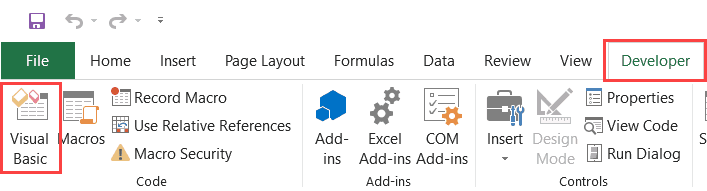
To open the Visual Basic Editor from the ribbon:
- Click the Developer tab (if you don’t see a developer tab, read this on how to get it).
- In the Code group, click on Visual Basic.
Using the Worksheet Tab
This is a less used method to open the Vb Editor.
Go to any of the worksheet tabs, right-click, and select ‘View Code’.
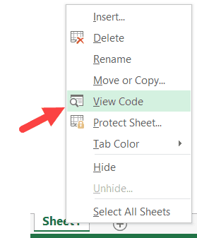
This method wouldn’t just open the VB Editor, it will also take you to the code window for that worksheet object.
This is useful when you want to write code that works only for a specific worksheet. This is usually the case with worksheet events.
Anatomy of the Visual Basic Editor in Excel
When you open the VB Editor for the first time, it may look a bit overwhelming.
There are different options and sections that may seem completely new at first.
Also, it still has an old Excel 97 days look. While Excel has improved tremendously in design and usability over the years, the VB Editor has not seen any change in the way it looks.
In this section, I will take you through the different parts of the Visual Basic Editor application.
Note: When I started using VBA years ago, I was quite overwhelmed with all these new options and windows. But as you get used to working with VBA, you would get comfortable with most of these. And most of the time, you’ll not be required to use all the options, only a hand full.
Below is an image of the different components of the VB Editor. These are then described in detail in the below sections of this tutorial.
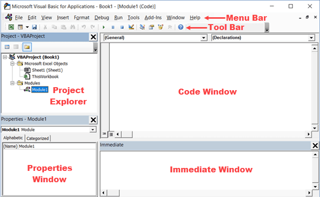
Now let’s quickly go through each of these components and understand what it does:
Menu Bar
This is where you have all the options that you can use in the VB Editor. It is similar to the Excel ribbon where you have tabs and options with each tab.
You can explore the available options by clicking on each of the menu element.
You will notice that most of the options in VB Editor have keyboard shortcuts mentioned next to it. Once you get used to a few keyboard shortcuts, working with the VB Editor becomes really easy.
Tool Bar
By default, there is a toolbar in the VB Editor which has some useful options that you’re likely to need most often. This is just like the Quick Access Toolbar in Excel. It gives you quick access to some of the useful options.
You can customize it a little by removing or adding options to it (by clicking on the small downward pointing arrow at the end of the toolbar).
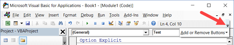
In most cases, the default toolbar is all you need when working with the VB Editor.
You can move the toolbar above the menu bar by clicking on the three gray dots (at the beginning of the toolbar) and dragging it above the menu bar.
Note: There are four toolbars in the VB Editor – Standard, Debug, Edit, and User form. What you see in the image above (which is also the default) is the standard toolbar. You can access other toolbars by going to the View option and hovering the cursor on the Toolbars option. You can add one or more toolbars to the VB Editor if you want.
Project Explorer
Project Explorer is a window on the left that shows all the objects currently open in Excel.
When you’re working with Excel, every workbook or add-in that is open is a project. And each of these projects can have a collection of objects in it.
For example, in the below image, the Project Explorer shows the two workbooks that are open (Book1 and Book2) and the objects in each workbook (worksheets, ThisWorkbook, and Module in Book1).
There is a plus icon to the left of objects that you can use to collapse the list of objects or expand and see the complete list of objects.
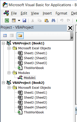
The following objects can be a part of the Project Explorer:
- All open Workbooks – within each workbook (which is also called a project), you can have the following objects:
- Worksheet object for each worksheet in the workbook
- ThisWorkbook object which represents the workbook itself
- Chartsheet object for each chart sheet (these are not as common as worksheets)
- Modules – This is where the code that is generated with a macro recorder goes. You can also write or copy-paste VBA code here.
- All open Add-ins
Consider the Project Explorer as a place that outlines all the objects open in Excel at the given time.
The keyboard shortcut to open the Project Explorer is Control + R (hold the control key and then press R). To close it, simply click the close icon at the top right of the Project Explorer window.
Note: For every object in Project Explorer, there is a code window in which you can write the code (or copy and paste it from somewhere). The code window appears when you double click on the object.
Properties Window
Properties window is where you get to see the properties of the select object. If you don’t have the Properties window already, you can get it by using the keyboard shortcut F4 (or go to the View tab and click Properties window).
Properties window is a floating window which you can dock in the VB Editor. In the below example, I have docked it just below the Project Explorer.
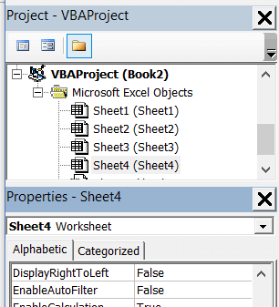
Properties window allows us to change the properties of a selected object. For example, if I want to make a worksheet hidden (or very hidden), I can do that by changing the Visible Property of the selected worksheet object.
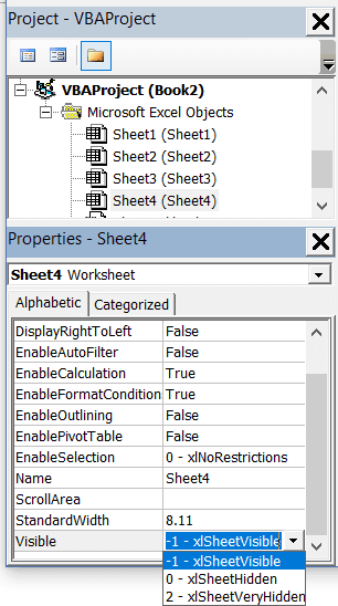
Related: Hiding a Worksheet in Excel (that can not be un-hidden easily)
Code Window
There is a code window for each object that is listed in the Project Explorer. You can open the code window for an object by double-clicking on it in the Project Explorer area.
Code window is where you’ll write your code or copy paste a code from somewhere else.
When you record a macro, the code for it goes into the code window of a module. Excel automatically inserts a module to place the code in it when recording a macro.
Related: How to Run a Macro (VBA Code) in Excel.
Immediate Window
The Immediate window is mostly used when debugging code. One way I use the Immediate window is by using a Print.Debug statement within the code and then run the code.
It helps me to debug the code and determine where my code gets stuck. If I get the result of Print.Debug in the immediate window, I know the code worked at least till that line.
If you’re new to VBA coding, it may take you some time to be able to use the immediate window for debugging.
By default, the immediate window is not visible in the VB Editor. You can get it by using the keyboard shortcut Control + G (or can go to the View tab and click on ‘Immediate Window’).
Where to Add Code in the VB Editor
I hope you now have a basic understanding of what VB Editor is and what all parts it has.
In this section of this tutorial, I will show you where to add a VBA code in the Visual Basic Editor.
There are two places where you can add the VBA code in Excel:
- The code window for an object. These objects can be a workbook, worksheet, User Form, etc.
- The code window of a module.
Module Code Window Vs Object Code Window
Let me first quickly clear the difference between adding a code in a module vs adding a code in an object code window.
When you add a code to any of the objects, it’s dependent on some action of that object that will trigger that code. For example, if you want to unhide all the worksheets in a workbook as soon as you open that workbook, then the code would go in the ThisWorkbook object (which represents the workbook).
The trigger, in this case, is opening the workbook.
Similarly, if you want to protect a worksheet as soon as some other worksheet is activated, the code for that would go in the worksheet code window.
These triggers are called events and you can associate a code to be executed when an event occurs.
Related: Learn more about Events in VBA.
On the contrary, the code in the module needs to be executed either manually (or it can be called from other subroutines as well).
When you record a macro, Excel automatically creates a module and inserts the recorded macro code in it. Now if you have to run this code, you need to manually execute the macro.
Adding VBA Code in Module
While recording a macro automatically creates a module and inserts the code in it, there are some limitations when using a macro recorder. For example, it can not use loops or If Then Else conditions.
In such cases, it’s better to either copy and paste the code manually or write the code yourself.
A module can be used to hold the following types of VBA codes:
- Declarations: You can declare variables in a module. Declaring variables allows you to specify what type of data a variable can hold. You can declare a variable for a sub-routine only or for all sub-routines in the module (or all modules)
- Subroutines (Procedures): This is the code that has the steps you want VBA to perform.
- Function Procedures: This is a code that returns a single value and you can use it to create custom functions (also called User Defined Functions or UDFs in VBA)
By default, a module is not a part of the workbook. You need to insert it first before using it.
Adding a Module in the VB Editor
Below are the steps to add a module:
- Right-click on any object of the workbook (in which you want the module).

- Hover the cursor on the Insert option.
- Click on Module.


This would instantly create a folder called Module and insert an object called Module 1. If you already have a module inserted, the above steps would insert another module.
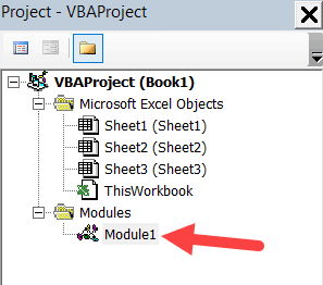
Once the module is inserted, you can double click on the module object in the Project Explorer and it will open the code window for it.
Now you can copy-paste the code or write it yourself.
Removing the Module
Below are the steps to remove a module in Excel VBA:
- Right-click on the module that you want to remove.
- Click on Remove Module option.

- In the dialog box that opens, click on No.


Note: You can export a module before removing it. It gets saved as a .bas file and you can import it in some other project. To export a module, right-click on the module and click on ‘Export file’.
Adding Code to the Object Code Window
To open the code window for an object, simply double-click on it.
When it opens, you can enter the code manually or copy-paste the code from other modules or from the internet.
Note that some of the objects allow you to choose the event for which you want to write the code.
For example, if you want to write a code for something to happen when selection is changed in the worksheet, you need to first select worksheets from the drop-down at the top left of the code window and then select the change event from the drop-down on the right.
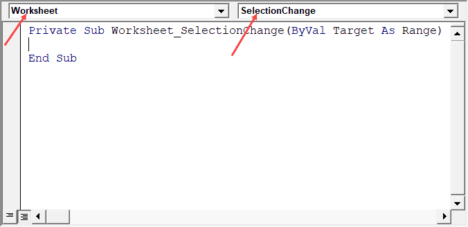
Note: These events are specific to the object. When you open the code window for a workbook, you will see the events related to the workbook object. When you open the code window for a worksheet, you will see the events related to the worksheet object.
Customizing the VB Editor
While the default settings of the Visual Basic Editor are good enough for most users, it does allow you to further customize the interface and a few functionalities.
In this section of the tutorial, I will show you all the options you have when customizing the VB Editor.
To customize the VB Editor environment, click Tools in the menu bar and then click on Options.
This would open the Options dialog box which will give you all the customization options in the VB Editor. The ‘Options’ dialog box has four tabs (as shown below) that have various customizations options for the Visual Basic Editor.
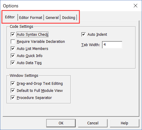
Let’s quickly go through each of these tabs and the important options in each.
Editor Tab
While the inbuilt settings work fine in most cases, let me still go through the options in this tab.
As you get more proficient working with VBA in Excel, you may want to customize the VB Editor using some of these options.
Auto Syntax Check
When working with VBA in Excel, as soon as you make a syntax error, you will be greeted by a pop-up dialog box (with some description about the error). Something as shown below:
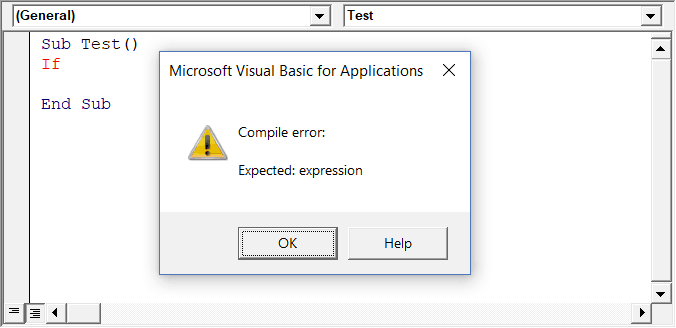
If you disable this option, this pop-up box will not appear even when you make a syntax error. However, there would be a change in color in the code text to indicate that there is an error.
If you’re a beginner, I recommend you keep this option enabled. As you get more experienced with coding, you may start finding these pop-up boxes irritating, and then you can disable this option.
Require Variable Declaration
This is one option I recommend enabling.
When you’re working with VBA, you would be using variables to hold different data types and objects.
When you enable this option, it automatically inserts the ‘Option Explicit’ statement at the top of the code window. This forces you to declare all the variables that you’re using in your code. If you don’t declare a variable and try to execute the code, it will show an error (as shown below).
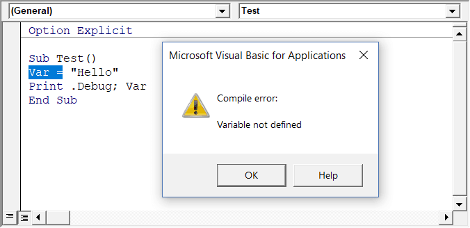
In the above case, I used the variable Var, but I didn’t declare it. So when I try to run the code, it shows an error.
This option is quite useful when you have a lot of variables. It often helps me find misspelled variables names as they are considered as undeclared and an error is shown.
Note: When you enable this option, it does not impact the existing modules.
Auto List Member
This option is quite useful as it helps you get a list of properties of methods for an object.
For example, if I want to delete a worksheet (Sheet1), I need to use the line Sheet1.Delete.
While I am typing the code, as soon as I type the dot, it will show me all the methods and properties associated with the Worksheet object (as shown below).
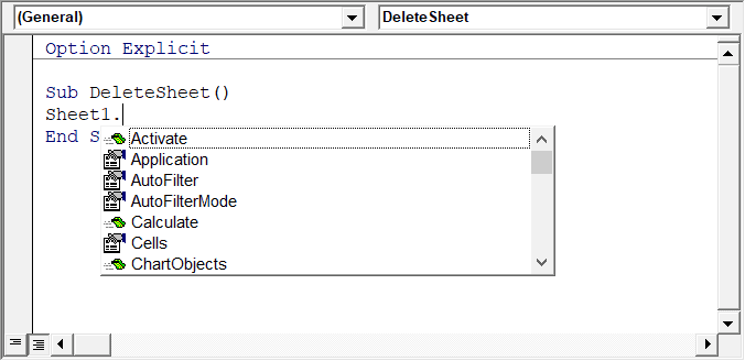
Auto list feature is great as it allows you to:
- Quickly select the property and method from the list and saves time
- Shows you all the properties and methods which you may not be aware of
- Avoid making spelling errors
This option is enabled by default and I recommend keeping it that way.
Auto Quick Info Options
When you type a function in Excel worksheet, it shows you some information about the function – such as the arguments it takes.
Similarly, when you type a function in VBA, it shows you some information (as shown below). But for that to happen, you need to make sure the Auto Quick Info option is enabled (which it is by default).
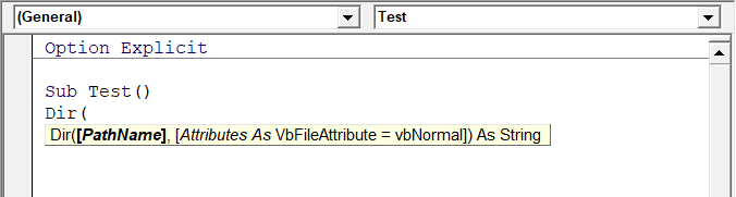
Auto Data Tips Options
When you’re going through your code line by line and place your cursor above a variable name, it will show you the value of the variable.
I find it quite useful when debugging the code or going through the code line by line which has loops in it.
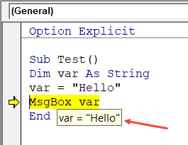
In the above example, as soon as I put the cursor over the variable (var), it shows the value it holds.
This option is enabled by default and I recommend you keep it that way.
Auto Indent
Since VBA codes can get long and messy, using indentation increases the readability of the code.
When writing code, you can indent using the tab key.
This option ensures that when you are done with the indented line and hit enter, the next line doesn’t start from the very beginning, but has the same indentation as the previous line.
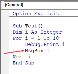
In the above example, after I write the Debug.Print line and hit enter, it will start right below it (with the same indentation level).
I find this option useful and turning this off would mean manually indenting each line in a block of code that I want indented.
You can change the indentation value if you want. I keep it at the default value.
Drag and Drop Text Editing
When this option is enabled, it allows you to select a block of code and drag and drop it.
It saves time as you don’t have to first cut and then paste it. You can simply select and drag it.
This option is enabled by default and I recommend you keep it that way.
Default to Full Module View
When this option is enabled, you will be able to see all the procedures in a module in one single scrollable list.
If you disable this option, you will only be able to see one module at a time. You will have to make a selection of the module you want to see from the drop-down at the top right of the code window.
This option is enabled by default and I recommend keeping it that way.
One reason you may want to disable it when you have multiple procedures that are huge and scrolling across these is taking time, or when you have a lot of procedures and you want to quickly find it instead of wasting time in scrolling.
Procedure Separator
When this option is enabled, you will see a line (a kind of divider) between two procedures.
I find this useful as it visually shows when one procedure ends and the other one starts.
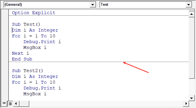
It’s enabled by default and I recommend keeping it that way.
Editor Format Tab
With the options in the Editor Format tab, you can customize the way your code looks in the code window.
Personally, I keep all the default options as I am fine with it. If you want, you can tweak this based on your preference.
To make a change, you need to first select an option in the Code Colors box. Once an option is selected, you can modify the foreground, background, and indicator color for it.
The font type and font size can also be set in this tab. It’s recommended to use a fixed-width font such as Courier New, as it makes the code more readable.
Note that the font type and size setting will remain the same for all code types (i.e., all the code types shown in the code color box).
Below is an image where I have selected Breakpoint, and I can change the formatting of it.
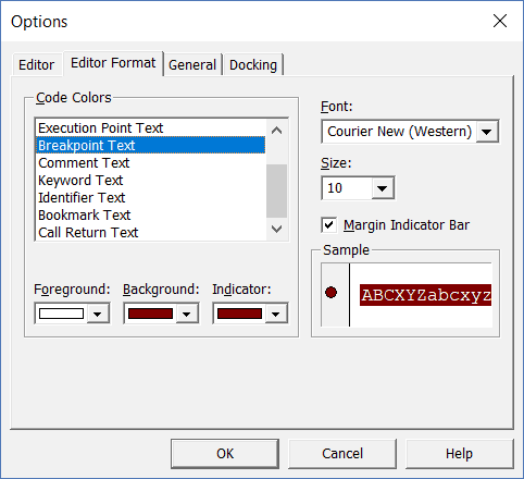
Note: The Margin Indicator Bar option when enabled shows a little margin bar to the left of the code. It’s helpful as it shows useful indicators when executing the code. In the above example, when you set a breakpoint, it will automatically show a red dot to the left of the line in the margin bar. Alternatively, to set a breakpoint, you can simply click on the margin bar on the left of the code line that you want as the breakpoint.
By default, Margin Indicator Bar is enabled and I recommend keeping it that way.
One of my VBA course students found this customization options useful and she was color blind. Using the options here, she was able to set the color and formats that made it easy for her to work with VBA.
General Tab
The General tab has many options but you don’t need to change any of it.
I recommend you keep all the options as is.
One important option to know about in this tab is Error Handling.
By default, ‘Break on Unhandled Errors’ is selected and I recommend keeping it that way.
This option means that if your code encounters an error, and you have not handled that error in your code already, then it will break and stop. But if you have addressed the error (such as by using On Error Resume Next or On Error Goto options), then it will not break (as the errors are not unhandled).
Docking Tab
In this tab, you can specify which windows you want to get docked.
Docking means that you can fix the position of a window (such as project explorer or the Properties window) so that it doesn’t float around and you can view all the different windows at the same time.
If you don’t dock, you will be able to view one window at a time in full-screen mode and will have to switch to the other one.
I recommend keeping the default settings.
Other Excel tutorials you may like:
- How to Remove Macros From an Excel Workbook
- Comments in Excel VBA (Add, Remove, Block Commenting)
- Using Active Cell in VBA in Excel (Examples)
The truth is: before you go for a job interview, you must have basic knowledge of Microsoft Excel. From an accountant to a receptionist, human resources to administration departments all are using Microsoft Excel.
It is not only limited to large companies, small entrepreneurs and college students are using it for their day-to-day work. That’s something that you can’t skip. To get a job, learning basic Excel tasks (at least some) is a must in today’s era, that’s a firm truth.
And, to help you with this I have compiled this guide. This guide will help you to learn all those basics using some examples. And some of the most important beginner’s tutorials.
So without further ado let’s get down to the business.
Introduction to Microsoft Excel
There is a number of spreadsheet programs but of all of them, Excel is the most widely used. People have been using it for the last 30 years and throughout these years, it has been upgraded with more and more features.
The best part about Excel is, that it can apply to many business tasks, including statistics, finance, data management, forecasting, analysis, tracking inventory & billing, and business intelligence. Following are the few things which it can do for you:
- Number Crunching
- Charts and Graphs
- Store and Import Data
- Manipulating Text
- Templates/Dashboards
- Automation of Tasks
- And Much More…
The three most important components of Excel you need to understand first:
1. Cell
A cell is a smallest but most powerful part of a spreadsheet. You can enter your data into a cell either by typing or by copy-paste. Data can be a text, a number, or a date. You can also customize it by changing its size, font color, background color, borders, etc. Every cell is identified by its cell address, cell address contains its column number and row number (If a cell is on the 11th row and on column AB, then its address will be AB11).
2. Worksheet:
A worksheet is made up of individual cells which can contain a value, a formula, or text. It also has an invisible draw layer, which holds charts, images, and diagrams. Each worksheet in a workbook is accessible by clicking the tab at the bottom of the workbook window. In addition, a workbook can store chart sheets; a chart sheet displays a single chart and is accessible by clicking a tab.
3. Workbook
A workbook is a separate file just like every other application has. Each workbook contains one or more worksheets. You can also say that a workbook is a collection of multiple worksheets or can be a single worksheet. You can add or delete worksheets, hide them within the workbook without deleting them, and change the order of your worksheets within the workbook.
Microsoft Excel Window Components
Before you start using it, it’s really important to understand what’s where in its window. So ahead we have all the major components which you need to know before entering the world of Microsoft Excel.

- Active Cell: A cell that is currently selected. It will be highlighted by a rectangular box and its address will be shown in the address bar. You can activate a cell by clicking on it or by using your arrow buttons. To edit a cell, you double-click on it or use F2 as well.
- Column: A column is a vertical set of cells. A single worksheet contains 16384 total columns. Every column has its own alphabet for identity, from A to XFD. You can select a column by clicking on its header.
- Row: A row is a horizontal set of cells. A single worksheet contains 1048576 total rows. Every row has its own number for identity, starting from 1 to 1048576. You can select a row by clicking on the row number marked on the left side of the window.
- Fill Handle: It’s a small dot present in the lower right corner of the active cell. It helps you to fill numeric values, text series, insert ranges, insert serial numbers, etc.
- Address Bar: It shows the address of the active cell. If you have selected more than one cell, then it will show the address of the first cell in the range.
- Formula Bar: The formula bar is an input bar, below the ribbon. It shows the content of the active cell and you can also use it to enter a formula in a cell.
- Title Bar: The title bar will show the name of your workbook, followed by the application name (“Microsoft Excel”).
- File Menu: The file menu is a simple menu like all other applications. It contains options like (Save, Save As, Open, New, Print, Excel Options, Share, etc).
- Quick Access Toolbar: A toolbar to quickly access the options which you frequently use. You can add your favorite options by adding new options to the quick access toolbar.
- Ribbon: Starting from Microsoft Excel 2007, all the options menus are replaced with ribbons. Ribbon tabs are a bunch of specific option group which further contains the option.
- Worksheet Tab: This tab shows all the worksheets which are present in the workbook. By default you will see, three worksheets in your new workbook with the names Sheet1, Sheet2, and Sheet3 respectively.
- Status Bar: It is a thin bar at the bottom of the Excel window. It will give you instant help once you start working in Excel.
Perform Basic Activities (Excel Knowledge Tutorials)
- Add and Delete a Worksheet in Excel
- Add and Remove Hyperlinks in Excel
- Add Watermark in Excel
- Apply Accounting Number Format in Excel
- Apply Background Color to a Cell or the Entire Sheet in Excel
- Delete Hidden Rows in Excel
- Deselect Cells in Excel
- Draw a Line in Excel
- Fill Justify in Excel to Merge Text from Multiple Cells
- Formula Bar in Excel (Hide, Unhide, and Expand)
- Print Excel Gridlines (Remove, Shortcut, & Change Color)
- Add a Button in Excel
- Add a Column in Excel
- Add a Header and Footer in Excel
- Add Page Number in Excel
- Apply Comma Style in Excel
- Apply Strikethrough in Excel
- Convert Negative Numbers into Positive in Excel
- Group Worksheets in the Excel
- Highlight Blank Cells in Excel
- Insert a Timestamp in Excel
- Insert Bullet Points in Excel
- Make Negative Numbers Red in Excel
- Merge – Unmerge Cells in Excel
- Rename Sheet in Excel
- Select Non-Contiguous Cells in Excel
- Show Ruler in Excel
- Spell Check in Excel
- Fill Handle in Excel
- Format Painter in Excel
- Move a Row and Column in Excel
- Excel Options (Mac and Windows)
- Add Border in Excel
- Change Border Color in Excel
- How to Change Column Width in Excel
- Clear Formatting in Excel
- View Two Sheets Side by Side in Excel
- Increase and Decrease Indent in Excel
- Insert an Arrow in a Cell in Excel
- Quick Access Toolbar in Excel
- Remove Pagebreak in Excel
- Rotate Text in Excel (Text Orientation)
- Row Vs Column in Excel (Difference)
- Automatically Add Serial Numbers in Excel
- Insert Delta Symbol in Excel in a Cell
- Insert (Type) Degree Symbol in Excel
- Top 10 Benefits of Microsoft Excel
- Set Print Area in Exm,cel
- Delete Blank Rows in Excel
- Convert a Formula to Value in Excel
- Excel for Accountants
- Sort By Date, Date, and Time & Reverse Date Sort in Excel
- Find and Replace in Excel
- Status Bar in Excel
- Make a Paragraph in a Cell in Excel
- Cell Style (Title, Calculation, Total, Headings…) in Excel
- Hide and Unhide a Workbook in Excel
- Change Date Format in Excel
- Center a Worksheet Horizontally and Vertically in Excel
- Make a Copy of the Excel Workbook (File)
- Write (Type) Vertically in Excel
- Insert Text Box in Excel
- Change Tab Color in Excel (Worksheet Tab Background Color)
- Delete a Single Row or Multiple Rows in Excel
- Copy and Paste a Column in Excel
- Zoom In or Zoom Out in Excel
- Copy Formatting in Excel
- How to Dialog Box in Excel
- How to Freeze Panes in Excel
- Insert a Check Mark Symbol [Tickmark] in Excel
- Quickly Swap Two Cells in Excel
Keyboard Shortcuts for Excel
Following are some of the useful keyboard shortcuts that you learn to perform activities quickly.
- Absolute Reference (Excel Shortcut)
- Add Column (Excel Shortcut)
- Add Comments (Excel Shortcut)
- Add Indent (Excel Shortcut)
- Add New Sheet (Excel Shortcut)
- Align Center (Excel Shortcut)
- Apply Border (Excel Shortcut)
- Apply and Remove Filter (Excel Shortcut)
- Auto Fit (Excel Shortcut)
- AutoSum (Excel Shortcut)
- Check Mark (Excel Shortcut)
- Clear Contents (Excel Shortcut)
- Close (Excel Shortcut)
- Copy and Paste (Excel Shortcut)
- Currency Format (Excel Shortcut)
- Cut and Paste (Excel Shortcut)
- Delete Cell (Excel Shortcut)
- Delete Row(s) (Excel Shortcut)
- Delete Sheet (Excel Shortcut)
- Drag Down (Excel Shortcut)
- Edit Cell (Excel Shortcut)
- Fill Color (Excel Shortcut)
- Find and Replace (Excel Shortcut)
- Format Painter (Excel Shortcut)
- Freeze Pane (Excel Shortcut)
- Full Screen (Excel Shortcut)
- Group (Excel Shortcut)
- Hyperlink (Excel Shortcut)
- Insert Cell (Excel Shortcut)
- Insert – Add Row(s) (Excel Shortcut)
- Lock Cells (Excel Shortcut)
- Merge-Unmerge Cells (Excel Shortcut)
- Open Format Cells Option (Excel Shortcut)
- Paste Values (Excel Shortcut)
- Percentage Format (Excel Shortcut)
- Print Preview (Excel Shortcut)
- Save As (Excel Shortcut)
- Select Row (Excel Shortcut)
- Show Formulas (Excel Shortcut)
- Strikethrough (Excel Shortcut)
- Subscript (Excel Shortcut)
- Superscript (Excel Shortcut)
- Switch Tabs (Excel Shortcut)
- Transpose (Excel Shortcut)
- Undo and Redo (Excel Shortcut)
- Unhide Columns (Excel Shortcut)
- Wrap Text (Excel Shortcut)
- Zoom-In (Excel Shortcut)
- Apply Date Format (Excel Shortcut)
- Apply Time Format (Excel Shortcut)
- Delete (Excel Shortcut)
- Open Go To Option (Excel Shortcut)
- Excel Date Functions
- Excel Financial Functions
- Excel Information Functions
- Excel Logical Functions
- Excel Lookup Functions
- Excel Math Functions
- Excel Statistical Functions
- Excel String (Text) Functions
- Excel Time Functions
- INT
- SUMPRODUCT
- MROUND
- MOD
- SUMIFS
- ABS
- SUMIF
- What is a Function in Excel
Recommended Books
Below are my two favorite Excel books for beginners which every person who is starting out with Excel should read.
- Excel 2016 for Dummies: This book covers everything you need to know to perform the task at hand. Includes information on creating and editing worksheets, formatting cells, and entering formulas […]
- Microsoft Excel 2016 Bible: Whether you are just starting out or an Excel novice, the Excel 2016 Bible is your comprehensive, go-to guide for all your Excel 2016 needs Whether you use Excel at work or […]
From Excel Basics to Advanced with In-Depth Guides and Tutorials
- Excel Formulas
- Pivot Table
- Excel Functions
- Power Query
- Excel for Accountants
- Benefits of Microsoft Excel
- VBA in Excel
- Excel Skills