
Total the data in an Excel table
You can quickly total data in an Excel table by enabling the Total Row option, and then use one of several functions that are provided in a drop-down list for each table column. The Total Row default selections use the SUBTOTAL function, which allow you to include or ignore hidden table rows, however you can also use other functions.

-
Click anywhere inside the table.
-
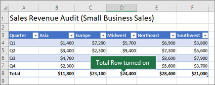
Go to Table Tools > Design, and select the check box for Total Row.

-
The Total Row is inserted at the bottom of your table.
Note: If you apply formulas to a total row, then toggle the total row off and on, Excel will remember your formulas. In the previous example we had already applied the SUM function to the total row. When you apply a total row for the first time, the cells will be empty.
-
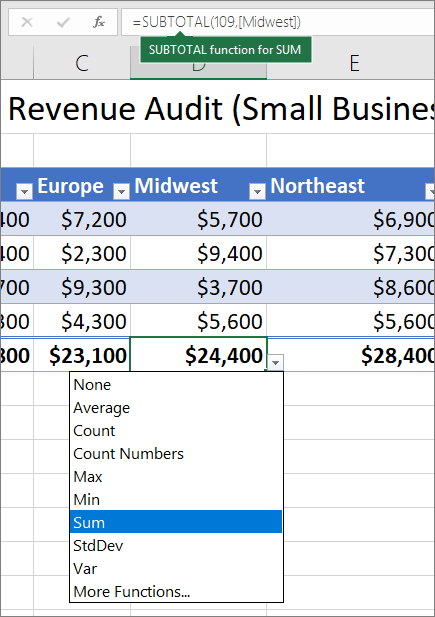
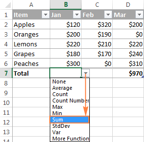
Select the column you want to total, then select an option from the drop-down list. In this case, we applied the SUM function to each column:
You’ll see that Excel created the following formula: =SUBTOTAL(109,[Midwest]). This is a SUBTOTAL function for SUM, and it is also a Structured Reference formula, which is exclusive to Excel tables. Learn more about Using structured references with Excel tables.
You can also apply a different function to the total value, by selecting the More Functions option, or writing your own.
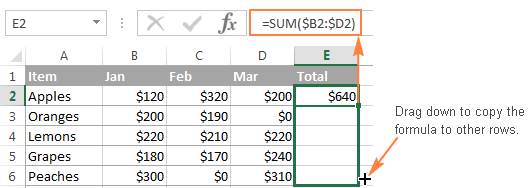
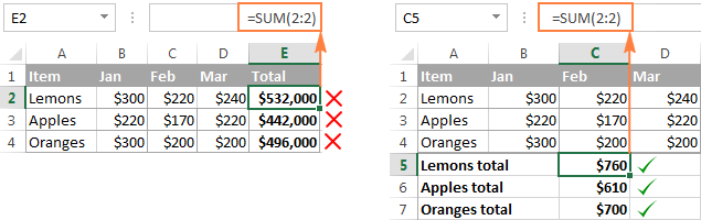
Note: If you want to copy a total row formula to an adjacent cell in the total row, drag the formula across using the fill handle. This will update the column references accordingly and display the correct value. If you copy and paste a formula in the total row, it will not update the column references as you copy across, and will result in inaccurate values.
You can quickly total data in an Excel table by enabling the Total Row option, and then use one of several functions that are provided in a drop-down list for each table column. The Total Row default selections use the SUBTOTAL function, which allow you to include or ignore hidden table rows, however you can also use other functions.
-
Click anywhere inside the table.
-
Go to Table > Total Row.
-
The Total Row is inserted at the bottom of your table.
Note: If you apply formulas to a total row, then toggle the total row off and on, Excel will remember your formulas. In the previous example we had already applied the SUM function to the total row. When you apply a total row for the first time, the cells will be empty.
-
Select the column you want to total, then select an option from the drop-down list. In this case, we applied the SUM function to each column:
You’ll see that Excel created the following formula: =SUBTOTAL(109,[Midwest]). This is a SUBTOTAL function for SUM, and it is also a Structured Reference formula, which is exclusive to Excel tables. Learn more about Using structured references with Excel tables.
You can also apply a different function to the total value, by selecting the More Functions option, or writing your own.
Note: If you want to copy a total row formula to an adjacent cell in the total row, drag the formula across using the fill handle. This will update the column references accordingly and display the correct value. If you copy and paste a formula in the total row, it will not update the column references as you copy across, and will result in inaccurate values.
You can quickly total data in an Excel table by enabling the Toggle Total Row option.
-
Click anywhere inside the table.
-
Click the Table Design tab > Style Options > Total Row.
The Total row is inserted at the bottom of your table.
Set the aggregate function for a Total Row cell
Note: This is one of several beta features, and currently only available to a portion of Office Insiders at this time. We’ll continue to optimize these features over the next several months. When they’re ready, we’ll release them to all Office Insiders, and Microsoft 365 subscribers.
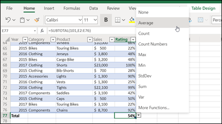
The Totals Row lets you pick which aggregate function to use for each column.
-
Click the cell in the Totals Row under the column you want to adjust, then click the drop-down that appears next to the cell.
-
Select an aggregate function to use for the column. Note that you can click More Functions to see additional options.
Need more help?
You can always ask an expert in the Excel Tech Community or get support in the Answers community.
See Also
Overview of Excel tables
Video: Create an Excel table
Create or delete an Excel table
Format an Excel table
Resize a table by adding or removing rows and columns
Filter data in a range or table
Convert a table to a range
Using structured references with Excel tables
Subtotal and total fields in a PivotTable report
Subtotal and total fields in a PivotTable
Excel table compatibility issues
Export an Excel table to SharePoint
Need more help?
Want more options?
Explore subscription benefits, browse training courses, learn how to secure your device, and more.
Communities help you ask and answer questions, give feedback, and hear from experts with rich knowledge.
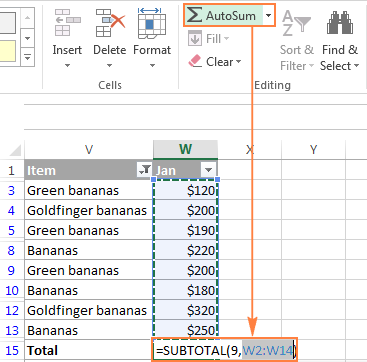
Select a cell next to the numbers you want to sum, click AutoSum on the Home tab, press Enter, and you’re done. When you click AutoSum, Excel automatically enters a formula (that uses the SUM function) to sum the numbers. Here’s an example.
Contents
- 1 How do you make a total row in Excel?
- 2 How do you add up cells in Excel?
- 3 How do I sum multiple rows and columns in Excel?
- 4 What is SUM function in Excel with example?
- 5 How do I create a formula for multiple cells in Excel?
- 6 How do I count cells in Excel?
- 7 How many columns Total Excel?
- 8 How do I get a running total in Excel with two columns?
- 9 How do you do a running total in numbers?
- 10 How do I total multiple rows in Excel?
- 11 How do you sum and group in Excel?
- 12 How do you sum multiple columns in Excel?
- 13 What is total row in Excel?
- 14 How do you sum subtotals in Excel?
- 15 How do you add subtotals using sum in Excel?
- 16 How do I count a list of names in Excel?
- 17 How do you SUM text in Excel?
- 18 What is a SUM example?
- 19 How many sheets can be created in Excel?
- 20 How do u calculate balance?
How do you make a total row in Excel?
Try it!
- Select a cell in a table.
- Select Design > Total Row.
- The Total row is added to the bottom of the table.
- From the total row drop-down, you can select a function, like Average, Count, Count Numbers, Max, Min, Sum, StdDev, Var, and more.
How do you add up cells in Excel?
AutoSum makes it easy to add adjacent cells in rows and columns. Click the cell below a column of adjacent cells or to the right of a row of adjacent cells. Then, on the HOME tab, click AutoSum, and press Enter. Excel adds all of the cells in the column or row.
How do I sum multiple rows and columns in Excel?
To do this:
- Select the data to sum plus the blank row below the data and the blank column to the right of the data where the totals will display.
- On the “Home” tab, in the “Editing” group, click the AutoSum button. Totals are calculated and appear in the last row and in the last column of the selected range!
What is SUM function in Excel with example?
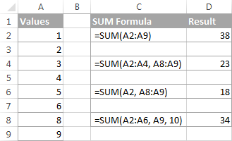
The SUM function adds values. You can add individual values, cell references or ranges or a mix of all three. For example: =SUM(A2:A10) Adds the values in cells A2:10. =SUM(A2:A10, C2:C10) Adds the values in cells A2:10, as well as cells C2:C10.
How do I create a formula for multiple cells in Excel?
Just select all the cells at the same time, then enter the formula normally as you would for the first cell. Then, when you’re done, instead of pressing Enter, press Control + Enter. Excel will add the same formula to all cells in the selection, adjusting references as needed.
How do I count cells in Excel?
Ways to count cells in a range of data
- Select the cell where you want the result to appear.
- On the Formulas tab, click More Functions, point to Statistical, and then click one of the following functions: COUNTA: To count cells that are not empty.
- Select the range of cells that you want, and then press RETURN.
How many columns Total Excel?
16,384 columns
Worksheet and workbook specifications and limits
| Feature | Maximum limit |
|---|---|
| Open workbooks | Limited by available memory and system resources |
| Total number of rows and columns on a worksheet | 1,048,576 rows by 16,384 columns |
| Column width | 255 characters |
| Row height | 409 points |
How do I get a running total in Excel with two columns?
Assuming your deposits start in cell A2 and payments in B2, you would enter the formula =SUBTOTAL(109,$A$2:A2,$B$2:B2) in C2 to start the running total. Use autofill to copy the formula down for each row. 109 represents the SUM function. $A$2:A2,$B$2:B2 are references to your deposit and payment columns.
How do you do a running total in numbers?
- A running total is the summation of a sequence of numbers which is updated each time a new number is added to the sequence, by adding the value of the new number to the previous running total. Another term for it is partial sum.
- Answer: 5 + 8 + 3 + 2 = 18.
- Answer: 5 + 8 + 3 + 2 + 6 = 24.
How do I total multiple rows in Excel?
Hold Ctrl + Shift key together and press Left Arrow. Close the bracket and hit the enter key to get the total. Similarly, we can add multiple rows together. Open SUM function in the G1 cell.
How do you sum and group in Excel?
You can sum values by group with one formula easily in Excel. Select next cell to the data range, type this =IF(A2=A1,””,SUMIF(A:A,A2,B:B)), (A2 is the relative cell you want to sum based on, A1 is the column header, A:A is the column you want to sum based on, the B:B is the column you want to sum the values.)
How do you sum multiple columns in Excel?
Type the formula =SUM($B:$D) in cell F11. This will sum up all the values of columns B, C and D. The usefulness of using this formula is that, whenever you will place new products name along with the sales value, it will get updated automatically if the new values are in this column range.
What is total row in Excel?
The Totals Row lets you pick which aggregate function to use for each column. Click the cell in the Totals Row under the column you want to adjust, then click the drop-down that appears next to the cell.
How do you sum subtotals in Excel?
Therefore, the solution is to use the Subtotal function, which only calculates the visible cells in a range.
- Display workbook in Excel containing data to be filtered.
- Click anywhere in the data set.
- Apply filter on data.
- Click below the data to sum.
- Enter the Subtotal formula to sum the filtered data.
How do you add subtotals using sum in Excel?
How to Insert Subtotals
- Select or highlight the worksheet data.
- Go to the Data menu in the ribbon.
- Look in the Outline grouping of commands.
- Click on the Subtotal command and you’ll notice a Subtotal dialogue box will open.
- In the Add subtotal to box, select Q1, Q2, Q3, Q4 and Year End.
How do I count a list of names in Excel?
Counting items in an Excel list
- Sort the list by the appropriate column.
- Use Advanced Filter to create a list of the unique entries in the appropriate column.
- Use the =Countif function to count the number of times each unique entry appears in the original list.
How do you SUM text in Excel?
In this article, we will learn how to Get the Sum of text values like numbers in Excel. In simple words, while working with text values in dataset.
What is a SUM example?
The definition of a sum is a total amount you arrive at by adding up multiple things, or the total amount of something that exists, or the total amount of money you have. 4 is an example of the sum of 2+2. When you have $100, this is an example of the sum of money that you have.
How many sheets can be created in Excel?
Although you’re limited to 255 sheets in a new workbook, Excel doesn’t limit how many worksheets you can add after you’ve created a workbook.
How do u calculate balance?
The daily or monthly average balance is calculated using multiple closing balances over the selected period of time. A simple average balance between a beginning and ending date is calculated by adding the beginning balance and the ending balance together, then dividing that amount by two.
Last Update: Jan 03, 2023
This is a question our experts keep getting from time to time. Now, we have got the complete detailed explanation and answer for everyone, who is interested!
Asked by: Augusta Ruecker
Score: 5/5
(41 votes)
Select a cell next to the numbers you want to sum, click AutoSum on the Home tab, press Enter, and you’re done. When you click AutoSum, Excel automatically enters a formula (that uses the SUM function) to sum the numbers.
How do I total a SUM in Excel?
To sum a range of cells, use the SUM function. To sum cells based on one criteria (for example, greater than 9), use the following SUMIF function (two arguments). To sum cells based on one criteria (for example, green), use the following SUMIF function (three arguments, last argument is the range to sum).
What is the formula for SUM in Excel?
The SUM function adds values. You can add individual values, cell references or ranges or a mix of all three. For example: =SUM(A2:A10) Adds the values in cells A2:10.
How do you total a row in Excel?
You can quickly total data in an Excel table by enabling the Toggle Total Row option.
- Click anywhere inside the table.
- Click the Table Design tab > Style Options > Total Row. The Total row is inserted at the bottom of your table.
How do I enable filtering?
Try it!
- Select any cell within the range.
- Select Data > Filter.
- Select the column header arrow .
- Select Text Filters or Number Filters, and then select a comparison, like Between.
- Enter the filter criteria and select OK.
22 related questions found
How do you create a formula for a column in Excel?
To insert a formula in Excel for an entire column of your spreadsheet, enter the formula into the topmost cell of your desired column and press «Enter.» Then, highlight and double-click the bottom-right corner of this cell to copy the formula into every cell below it in the column.
What is Excel average formula?
Description. Returns the average (arithmetic mean) of the arguments. For example, if the range A1:A20 contains numbers, the formula =AVERAGE(A1:A20) returns the average of those numbers.
How many Excel formulas are there?
Excel has over 475 formulas in its Functions Library, from simple mathematics to very complex statistical, logical, and engineering tasks such as IF statements (one of our perennial favorite stories); AND, OR, NOT functions; COUNT, AVERAGE, and MIN/MAX.
Which formula is not entered correctly?
Solution(By Examveda Team)
A formula always starts with an equal sign (=), which can be followed by numbers, math operators (such as a plus or minus sign), and functions, which can really expand the power of a formula. Here in option D 10+50 there is no equal sign (=), so it is not correct.
What is count A in Excel?
Description. The COUNTA function counts the number of cells that are not empty in a range.
Is there a Sumif function in Excel?
The Excel SUMIF function returns the sum of cells that meet a single condition. Criteria can be applied to dates, numbers, and text. The SUMIF function supports logical operators (>,<,<>,=) and wildcards (*,?) for partial matching.
How do you create spreadsheet?
Open a new, blank workbook
- Click the File tab.
- Click New.
- Under Available Templates, double-click Blank Workbook. Keyboard shortcut To quickly create a new, blank workbook, you can also press CTRL+N.
Which symbol is entered before a formula?
If you type in the formula, you must start with an equal sign, so Excel knows that the data in the cell is a formula. After the =, what comes next depends on what you’re trying to do. If you are multiplying numbers, just type in the appropriate numbers and mathematical symbol (* for multiply).
Which is not a function in MS Excel?
The correct answer to the question “Which one is not a function in MS Excel” is option (b). AVG. There is no function in Excel like AVG, at the time of writing, but if you mean Average, then the syntax for it is also AVERAGE and not AVG. The other two options are correct.
How can u activate a cell?
Answer: D. A cell can be ready to activate by any of the method Pressing the Tab key or Clicking the cell or Pressing an arrow key.
What are the 5 functions in Excel?
To help you get started, here are 5 important Excel functions you should learn today.
- The SUM Function. The sum function is the most used function when it comes to computing data on Excel. …
- The TEXT Function. …
- The VLOOKUP Function. …
- The AVERAGE Function. …
- The CONCATENATE Function.
What is basic formula?
Formula is an expression that calculates values in a cell or in a range of cells. For example, =A2+A2+A3+A4 is a formula that adds up the values in cells A2 through A4. Function is a predefined formula already available in Excel.
What are the top 10 Excel formulas?
Top 10 Most Useful Excel Formulas
- SUM, COUNT, AVERAGE. SUM allows you to sum any number of columns or rows by selecting them or typing them in, for example, =SUM(A1:A8) would sum all values in between A1 and A8 and so on. …
- IF STATEMENTS.
- SUMIF, COUNTIF, AVERAGEIF.
- VLOOKUP. …
- CONCATENATE. …
- MAX & MIN. …
- AND. …
- PROPER.
What is grade formula Excel?
To find the grade, multiply the grade for each assignment against the weight, and then add these totals all up. … So for each cell (in the Total column) we will enter =SUM(Grade Cell * Weight Cell), so my first formula is =SUM(B2*C2), the next one would be =SUM(B3*C3) and so on.
What is Max function in Excel?
The Excel MAX function returns the largest numeric value in a range of values. The MAX function ignores empty cells, the logical values TRUE and FALSE, and text values. Get the largest value. The largest value in the array.
How do I automatically apply formulas in Excel without dragging?
Simply do the following:
- Select the cell with the formula and the adjacent cells you want to fill.
- Click Home > Fill, and choose either Down, Right, Up, or Left. Keyboard shortcut: You can also press Ctrl+D to fill the formula down in a column, or Ctrl+R to fill the formula to the right in a row.
How do I add a formula to existing data in Excel?
Just select all the cells at the same time, then enter the formula normally as you would for the first cell. Then, when you’re done, instead of pressing Enter, press Control + Enter. Excel will add the same formula to all cells in the selection, adjusting references as needed.
How do I do a percentage formula in Excel?
The percentage formula in Excel is = Numerator/Denominator (used without multiplication by 100). To convert the output to a percentage, either press “Ctrl+Shift+%” or click “%” on the Home tab’s “number” group.
Can you start a formula in Excel with?
Simple formulas always start with an equal sign (=), followed by constants that are numeric values and calculation operators such as plus (+), minus (-), asterisk(*), or forward slash (/) signs. Let’s take an example of a simple formula. On the worksheet, click the cell in which you want to enter the formula.
Contents
- 1 How do you total a column in Excel?
- 2 How do you total a row in Excel?
- 3 How do you total items in Excel?
- 4 Is there a total function in Excel?
- 5 How do I do a Sumif in Excel?
- 6 How do I calculate percentage of a total?
- 7 What is a formula of percentage?
- 8 How do you add 10% in Excel?
- 9 How do you find 5% of a number?
- 10 How do you calculate a 5% increase?
- 11 How do you calculate a 6% increase?
How do you total a column in Excel?
How to total columns in Excel with AutoSum
- Navigate to the Home tab -> Editing group and click on the AutoSum button.
- You will see Excel automatically add the =SUM function and pick the range with your numbers.
- Just press Enter on your keyboard to see the column totaled in Excel.
How do you total a row in Excel?
Select a cell in a table. Select Design > Total Row. The Total row is added to the bottom of the table. Note: To add a new row, uncheck the Total Row checkbox, add the row, and then recheck the Total Row checkbox.
How do you total items in Excel?
Ways to count cells in a range of data
- Select the cell where you want the result to appear.
- On the Formulas tab, click More Functions, point to Statistical, and then click one of the following functions: COUNTA: To count cells that are not empty. COUNT: To count cells that contain numbers.
- Select the range of cells that you want, and then press RETURN.
Is there a total function in Excel?
Go to Table > Total Row. The Total Row is inserted at the bottom of your table. Note: If you apply formulas to a total row, then toggle the total row off and on, Excel will remember your formulas.
How do I do a Sumif in Excel?
If you want, you can apply the criteria to one range and sum the corresponding values in a different range. For example, the formula =SUMIF(B2:B5, “John”, C2:C5) sums only the values in the range C2:C5, where the corresponding cells in the range B2:B5 equal “John.”
How do I calculate percentage of a total?
How to calculate percentage
- Determine the whole or total amount of what you want to find a percentage for.
- Divide the number that you wish to determine the percentage for.
- Multiply the value from step two by 100.
What is a formula of percentage?
The percentage tells you how number A relates to number B . To calculate the percentage, multiply this fraction by 100 and add a percent sign. 100 * numerator / denominator = percentage . In our example it’s 100 * 2/5 = 100 * 0.4 = 40 .
How do you add 10% in Excel?
To increase a number by a percentage amount, multiply the original amount by 1+ the percent of increase. In the example shown, Product A is getting a 10 percent increase. So you first add 1 to the 10 percent, which gives you 110 percent. You then multiply the original price of 100 by 110 percent.
How do you find 5% of a number?
How do you calculate a 5% increase?
How to calculate percent increase. Percent increase formula. Calculating percent decrease.
How do I add 5% to a number?
- Divide the number you wish to add 5% to by 100.
- Multiply this new number by 5.
- Add the product of the multiplication to your original number.
- Enjoy working at 105%!
How do you calculate a 6% increase?
Detailed calculations & verification
- Detailed calculations & verification. Introduction.
- Increase the number by 6% of its value. Percentage increase = 6% × 100.
- Calculate the New Value. New value =
- Calculate absolute change (actual difference) Absolute change (actual difference) =
- Proof. Calculate percentage increase:
Asked by: Augusta Ruecker
Score: 5/5
(41 votes)
Select a cell next to the numbers you want to sum, click AutoSum on the Home tab, press Enter, and you’re done. When you click AutoSum, Excel automatically enters a formula (that uses the SUM function) to sum the numbers.
How do I total a SUM in Excel?
To sum a range of cells, use the SUM function. To sum cells based on one criteria (for example, greater than 9), use the following SUMIF function (two arguments). To sum cells based on one criteria (for example, green), use the following SUMIF function (three arguments, last argument is the range to sum).
What is the formula for SUM in Excel?
The SUM function adds values. You can add individual values, cell references or ranges or a mix of all three. For example: =SUM(A2:A10) Adds the values in cells A2:10.
How do you total a row in Excel?
You can quickly total data in an Excel table by enabling the Toggle Total Row option.
- Click anywhere inside the table.
- Click the Table Design tab > Style Options > Total Row. The Total row is inserted at the bottom of your table.
How do I enable filtering?
Try it!
- Select any cell within the range.
- Select Data > Filter.
- Select the column header arrow .
- Select Text Filters or Number Filters, and then select a comparison, like Between.
- Enter the filter criteria and select OK.
22 related questions found
How do you create a formula for a column in Excel?
To insert a formula in Excel for an entire column of your spreadsheet, enter the formula into the topmost cell of your desired column and press «Enter.» Then, highlight and double-click the bottom-right corner of this cell to copy the formula into every cell below it in the column.
What is Excel average formula?
Description. Returns the average (arithmetic mean) of the arguments. For example, if the range A1:A20 contains numbers, the formula =AVERAGE(A1:A20) returns the average of those numbers.
How many Excel formulas are there?
Excel has over 475 formulas in its Functions Library, from simple mathematics to very complex statistical, logical, and engineering tasks such as IF statements (one of our perennial favorite stories); AND, OR, NOT functions; COUNT, AVERAGE, and MIN/MAX.
Which formula is not entered correctly?
Solution(By Examveda Team)
A formula always starts with an equal sign (=), which can be followed by numbers, math operators (such as a plus or minus sign), and functions, which can really expand the power of a formula. Here in option D 10+50 there is no equal sign (=), so it is not correct.
What is count A in Excel?
Description. The COUNTA function counts the number of cells that are not empty in a range.
Is there a Sumif function in Excel?
The Excel SUMIF function returns the sum of cells that meet a single condition. Criteria can be applied to dates, numbers, and text. The SUMIF function supports logical operators (>,<,<>,=) and wildcards (*,?) for partial matching.
How do you create spreadsheet?
Open a new, blank workbook
- Click the File tab.
- Click New.
- Under Available Templates, double-click Blank Workbook. Keyboard shortcut To quickly create a new, blank workbook, you can also press CTRL+N.
Which symbol is entered before a formula?
If you type in the formula, you must start with an equal sign, so Excel knows that the data in the cell is a formula. After the =, what comes next depends on what you’re trying to do. If you are multiplying numbers, just type in the appropriate numbers and mathematical symbol (* for multiply).
Which is not a function in MS Excel?
The correct answer to the question “Which one is not a function in MS Excel” is option (b). AVG. There is no function in Excel like AVG, at the time of writing, but if you mean Average, then the syntax for it is also AVERAGE and not AVG. The other two options are correct.
How can u activate a cell?
Answer: D. A cell can be ready to activate by any of the method Pressing the Tab key or Clicking the cell or Pressing an arrow key.
What are the 5 functions in Excel?
To help you get started, here are 5 important Excel functions you should learn today.
- The SUM Function. The sum function is the most used function when it comes to computing data on Excel. …
- The TEXT Function. …
- The VLOOKUP Function. …
- The AVERAGE Function. …
- The CONCATENATE Function.
What is basic formula?
Formula is an expression that calculates values in a cell or in a range of cells. For example, =A2+A2+A3+A4 is a formula that adds up the values in cells A2 through A4. Function is a predefined formula already available in Excel.
What are the top 10 Excel formulas?
Top 10 Most Useful Excel Formulas
- SUM, COUNT, AVERAGE. SUM allows you to sum any number of columns or rows by selecting them or typing them in, for example, =SUM(A1:A8) would sum all values in between A1 and A8 and so on. …
- IF STATEMENTS.
- SUMIF, COUNTIF, AVERAGEIF.
- VLOOKUP. …
- CONCATENATE. …
- MAX & MIN. …
- AND. …
- PROPER.
What is grade formula Excel?
To find the grade, multiply the grade for each assignment against the weight, and then add these totals all up. … So for each cell (in the Total column) we will enter =SUM(Grade Cell * Weight Cell), so my first formula is =SUM(B2*C2), the next one would be =SUM(B3*C3) and so on.
What is Max function in Excel?
The Excel MAX function returns the largest numeric value in a range of values. The MAX function ignores empty cells, the logical values TRUE and FALSE, and text values. Get the largest value. The largest value in the array.
How do I automatically apply formulas in Excel without dragging?
Simply do the following:
- Select the cell with the formula and the adjacent cells you want to fill.
- Click Home > Fill, and choose either Down, Right, Up, or Left. Keyboard shortcut: You can also press Ctrl+D to fill the formula down in a column, or Ctrl+R to fill the formula to the right in a row.
How do I add a formula to existing data in Excel?
Just select all the cells at the same time, then enter the formula normally as you would for the first cell. Then, when you’re done, instead of pressing Enter, press Control + Enter. Excel will add the same formula to all cells in the selection, adjusting references as needed.
How do I do a percentage formula in Excel?
The percentage formula in Excel is = Numerator/Denominator (used without multiplication by 100). To convert the output to a percentage, either press “Ctrl+Shift+%” or click “%” on the Home tab’s “number” group.
Can you start a formula in Excel with?
Simple formulas always start with an equal sign (=), followed by constants that are numeric values and calculation operators such as plus (+), minus (-), asterisk(*), or forward slash (/) signs. Let’s take an example of a simple formula. On the worksheet, click the cell in which you want to enter the formula.
Содержание
- Total the data in an Excel table
- Set the aggregate function for a Total Row cell
- Need more help?
- Excel SUM formula to total a column, rows or only visible cells
- How to sum in Excel using a simple arithmetic calculation
- How to use SUM function in Excel
- How to AutoSum in Excel
- How to sum a column in Excel
- Total an entire column with indefinite number of rows
- Sum column except header or excluding a few first rows
- How to sum rows in Excel
- How to sum multiple rows in Excel
- How to sum a whole row
- Use Excel Total Row to sum data in a table
- How to add a total row in Excel tables
- How to total data in your table
- How to sum only filtered (visible) cells in Excel
- How to do a running total (cumulative sum) in Excel
- How to sum across sheets
- Excel conditional sum
- Excel SUM not working — reasons and solutions
- 1. #Name error appears instead of the expected result
- 2. Some numbers are not added
- 3. Excel SUM function returns 0
- 4. Excel Sum formula returns a higher number than expected
- 5. Excel SUM formula not updating
- Practice workbook for download
- You may also be interested in
Total the data in an Excel table
You can quickly total data in an Excel table by enabling the Total Row option, and then use one of several functions that are provided in a drop-down list for each table column. The Total Row default selections use the SUBTOTAL function, which allow you to include or ignore hidden table rows, however you can also use other functions.
Click anywhere inside the table.
Go to Table Tools > Design, and select the check box for Total Row.

The Total Row is inserted at the bottom of your table.
Note: If you apply formulas to a total row, then toggle the total row off and on, Excel will remember your formulas. In the previous example we had already applied the SUM function to the total row. When you apply a total row for the first time, the cells will be empty.
Select the column you want to total, then select an option from the drop-down list. In this case, we applied the SUM function to each column:
You’ll see that Excel created the following formula: =SUBTOTAL(109,[Midwest]). This is a SUBTOTAL function for SUM, and it is also a Structured Reference formula, which is exclusive to Excel tables. Learn more about Using structured references with Excel tables.
You can also apply a different function to the total value, by selecting the More Functions option, or writing your own.
Note: If you want to copy a total row formula to an adjacent cell in the total row, drag the formula across using the fill handle. This will update the column references accordingly and display the correct value. If you copy and paste a formula in the total row, it will not update the column references as you copy across, and will result in inaccurate values.
You can quickly total data in an Excel table by enabling the Total Row option, and then use one of several functions that are provided in a drop-down list for each table column. The Total Row default selections use the SUBTOTAL function, which allow you to include or ignore hidden table rows, however you can also use other functions.
Click anywhere inside the table.
Go to Table > Total Row.
The Total Row is inserted at the bottom of your table.
Note: If you apply formulas to a total row, then toggle the total row off and on, Excel will remember your formulas. In the previous example we had already applied the SUM function to the total row. When you apply a total row for the first time, the cells will be empty.
Select the column you want to total, then select an option from the drop-down list. In this case, we applied the SUM function to each column:
You’ll see that Excel created the following formula: =SUBTOTAL(109,[Midwest]). This is a SUBTOTAL function for SUM, and it is also a Structured Reference formula, which is exclusive to Excel tables. Learn more about Using structured references with Excel tables.
You can also apply a different function to the total value, by selecting the More Functions option, or writing your own.
Note: If you want to copy a total row formula to an adjacent cell in the total row, drag the formula across using the fill handle. This will update the column references accordingly and display the correct value. If you copy and paste a formula in the total row, it will not update the column references as you copy across, and will result in inaccurate values.
You can quickly total data in an Excel table by enabling the Toggle Total Row option.
Click anywhere inside the table.
Click the Table Design tab > Style Options > Total Row.
The Total row is inserted at the bottom of your table.
Set the aggregate function for a Total Row cell
Note: This is one of several beta features, and currently only available to a portion of Office Insiders at this time. We’ll continue to optimize these features over the next several months. When they’re ready, we’ll release them to all Office Insiders, and Microsoft 365 subscribers.
The Totals Row lets you pick which aggregate function to use for each column.
Click the cell in the Totals Row under the column you want to adjust, then click the drop-down that appears next to the cell.
Select an aggregate function to use for the column. Note that you can click More Functions to see additional options.
Need more help?
You can always ask an expert in the Excel Tech Community or get support in the Answers community.
Источник
Excel SUM formula to total a column, rows or only visible cells
 by Svetlana Cheusheva, updated on March 7, 2023
The tutorial explains how to do sum in Excel by using the AutoSum feature, and how to make your own SUM formula to total a column, row or selected range. You will also learn how to sum only visible cells, calculate running total, sum across sheets, and find out why your Excel Sum formula is not working.
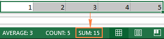
If you want a quick sum of certain cells in Excel, you can simply select those cells, and look at the status bar at the bottom right corner of your Excel window:
For something more permanent, use the Excel SUM function. It is very simple and straightforward, so even if you are a beginner in Excel, you will hardly have any difficulty in understanding the following examples.
How to sum in Excel using a simple arithmetic calculation
If you need a quick total of several cells, you can use Microsoft Excel as a mini calculator. Just utilize the plus sign operator (+) like in a normal arithmetic operation of addition. For example:
However, if you need to sum a few dozen or a few hundred rows, referencing each cell in a formula does not sound like a good idea. In this case, you can use the Excel SUM function specially designed to add a specified set of numbers.
How to use SUM function in Excel
Excel SUM is a math and trig function that adds values. The syntax of the SUM function is as follows:
The first argument is required, other numbers are optional, and you can supply up to 255 numbers in a single formula.
In your Excel SUM formula, each argument can be a positive or negative numeric value, range, or cell reference. For example:
The Excel SUM function is useful when you need to add up values from different ranges, or combine numeric values, cell references and ranges. For example:
The below screenshot shows these and a few more SUM formula examples:
In real-life worksheets, the Excel SUM function is often included in bigger formulas as part of more complex calculations.
For example, you can embed SUM in the value_if_true argument of the IF function to add numbers in columns B, C and D if all three cells in the same row contain values, and show a warning message if any of the cells is blank:
=IF(AND($B2 «», $D2<>«»), SUM($B2:$D2), «Value missing»)
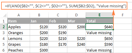
And here’s another example of using an advanced SUM formula in Excel: VLOOKUP and SUM formula to total all matching values.
How to AutoSum in Excel
If you need to sum one range of numbers, whether a column, row or several adjacent columns or rows, you can let Microsoft Excel write an appropriate SUM formula for you.
Simply select a cell next to the numbers you want to add, click AutoSum on the Home tab, in the Editing group, press the Enter key, and you will have a Sum formula inserted automatically:
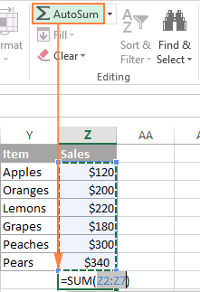
As you can see in the following screenshot, Excel’s AutoSum feature not only enters a Sum formula, but also selects the most likely range of cells that you’d want to total. Nine times out of ten, Excel gets the range right. If not, you can manually correct the range by simply dragging the cursor through the cells to sum, and then hit the Enter key.
Tip. A faster way to do AutoSum in Excel is to use the Sum shortcut Alt + = . Just hold the Alt key, press the Equal Sign key, and then hit Enter to complete an automatically inserted Sum formula.
Apart from calculating total, you can use AutoSum to automatically enter AVERAGE, COUNT, MAX, or MIN functions. For more information, please check out the Excel AutoSum tutorial.
How to sum a column in Excel
To sum numbers in a specific column, you can use either the Excel SUM function or AutoSum feature.
For example, to sum values in column B, say in cells B2 to B8, enter the following Excel SUM formula:
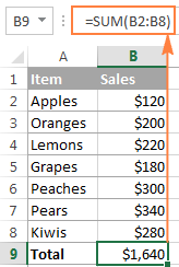
Total an entire column with indefinite number of rows
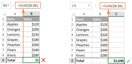
If a column you want to sum has a variable number of rows (i.e. new cells can be added and existing ones can be deleted at any time), you can sum the entire column by supplying a column reference, without specifying a lower or upper bound. For example:
Important note! In no case you should put your ‘Sum of a column’ formula in the column you want to total because this would create a circular cell reference (i.e. an endless recursive summation), and your Sum formula would return 0.
Sum column except header or excluding a few first rows
Usually, supplying a column reference to the Excel Sum formula totals the entire column ignoring the header, as demonstrated in the above screenshot. But in some cases, the header of the column you want to total can actually have a number in it. Or, you may want to exclude the first few rows with numbers that are not relevant to the data you want to sum.
Regrettably, Microsoft Excel does not accept a mixed SUM formula with an explicit lower bound but without an upper bound like =SUM(B2:B), which works fine in Google Sheets. To exclude the first few rows from summation, you can use one of the following workarounds.
- Sum the entire column and then subtract the cells you don’t want to include in the total (cells B1 to B3 in this example):
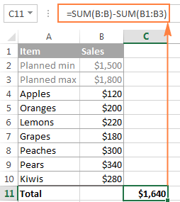
For example, to sum column B without the header (i.e. excluding cell B1), you can use the following formulas:
- In Excel 2007, Excel 2010, Excel 2013, and Excel 2016:
=SUM(B2:B1048576) - In Excel 2003 and lower:
=SUM(B2:B655366)
How to sum rows in Excel
Similarly to totaling a column, you can sum a row in Excel by using the SUM function, or have AutoSum to insert the formula for you.
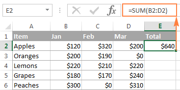
For example, to add values in cells B2 to D2, use the following formula:
How to sum multiple rows in Excel
To add values in each row individually, just drag down your Sum formula. The key point is to use relative (without $) or mixed cell references (where the $ sign fixes only the columns). For example:
To total the values in a range containing several rows, simply specify the desired range in the Sum formula. For example:
=SUM(B2:D6) — sums values in rows 2 to 6.
=SUM(B2:D3, B5:D6) — sums values in rows 2, 3, 5 and 6.
How to sum a whole row
To sum the entire row with an indefinite number of columns, supply a whole-row reference to your Excel Sum formula, e.g.:
Please remember that you shouldn’t enter that ‘Sum of a row’ formula in any cell of the same row to avoid creating a circular reference because this would result in a wrong calculation, if any:
To sum rows excluding a certain column(s), total the entire row and then subtract irrelevant columns. For example, to sum row 2 except the first 2 columns, use the following formula:
Use Excel Total Row to sum data in a table
If your data is organized in an Excel table, you can benefit from the special Total Row feature that can quickly sum the data in your table and display totals in the last row.
A big advantage of using Excel tables is that they auto-expand to include new rows, so any new data you input in a table will be included in your formulas automatically. If can learn about other benefits of Excel tables in this article: 10 most useful features of Excel tables.
To convert an ordinary range of cells into a table, select it and press Ctrl + T shortcut (or click Table on the Insert tab).
How to add a total row in Excel tables
Once your data is arranged in a table, you can insert a total row in this way:
- Click anywhere in the table to display the Table Tools with the Design tab.
- On the Design tab, in the Table Style Options group, select the Total Row box:

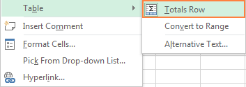
Another way to add a total row in Excel is to right click any cell within the table, and then click Table > Totals Row.
How to total data in your table
When the total row appears at the end of the table, Excel does its best to determine how you would like to calculate data in the table.
In my sample table, the values in column D (rightmost column) are added automatically and the sum is displayed in the Total Row:
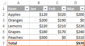
To total values in other columns, simply select a corresponding cell in the total row, click the drop-down list arrow, and select Sum:
If you want to perform some other calculation, select the corresponding function from the drop-down list such as Average, Count, Max, Min, etc.
If the total row automatically displays a total for a column that doesn’t need one, open the dropdown list for that column and select None.
Note. When using the Excel Total Row feature to sum a column, Excel totals values only in visible rows by inserting the SUBTOTAL function with the first argument set to 109. You will find the detailed explanation of this function in the next section.
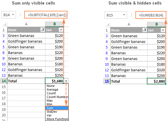
If you want to sum data both in visible and invisible rows, do not add the total row, and use a normal SUM function instead:
How to sum only filtered (visible) cells in Excel
Sometimes, for more effective date analysis, you may need to filter or hide some data in your worksheet. A usual Sum formula won’t work in this case because the Excel SUM function adds all values in the specified range including the hidden (filtered out) rows.
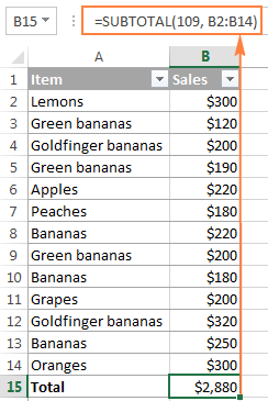
If you want to sum only visible cells in a filtered list, the fastest way is to organize your data in an Excel table, and then turn on the Excel Total Row feature. As demonstrated in the previous example, selecting Sum in a table’s total row inserts the SUBTOTAL function that ignores hidden cells.
Another way to sum filtered cells in Excel is to apply an AutoFilter to your data manually by clicking the Filter button on the Data tab. And then, write a Subtotal formula yourself.
The SUBTOTAL function has the following syntax:
- Function_num— a number from 1 to 11 or from 101 to 111 that specifies which function to use for the subtotal.
You can find the full list of functions on support.office.com. For now, we are interested only in the SUM function, which is defined by numbers 9 and 109. Both numbers exclude filtered-out rows. The difference is that 9 includes cells hidden manually (i.e. right-click > Hide), while 109 excludes them.
So, if you are looking to sum only visible cells, regardless of how exactly irrelevant rows were hidden, then use 109 in the first argument of your Subtotal formula.
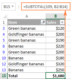
In this example, let’s sum visible cells in range B2:B14 by using the following formula:
And now, let’s filter only ‘Banana‘ rows and make sure that our Subtotal formula sums only visible cells:
Tip. You can have Excel’s AutoSum feature to insert the Subtotal formula for you automatically. Just organize your data in table ( Ctrl + T ) or filter the data the way you want by clicking the Filter button. After that, select the cell immediately below the column you want to total, and click the AutoSum button on the ribbon. A SUBTOTAL formula will be inserted, summing only the visible cells in the column.
How to do a running total (cumulative sum) in Excel
To calculate a running total in Excel, you write a usual SUM formula with a clever use of absolute and relative cells references.
For example, to display the cumulative sum of numbers in column B, enter the following formula in C2, and then copy it down to other cells:
The relative reference B2 will change automatically based on the relative position of the row in which the formula is copied:
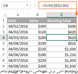
You can find the detailed explanation of this basic Cumulative Sum formula and tips on how to improve it in this tutorial: How to calculate running total in Excel.
How to sum across sheets
If you have several worksheets with the same layout and the same data type, you can add the values in the same cell or in the same range of cells in different sheets with a single SUM formula.
A so-called 3-D reference is what does the trick:
The first formula adds values in cell B6, while the second formula sums the range B2:B5 in all worksheets located between the two boundary sheets that you specify (Jan and Apr in this example):
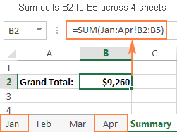
You can find more information about a 3-d reference and the detailed steps to create such formulas in this tutorial: How to create a 3-D reference to calculate multiple sheets.
Excel conditional sum
If your task requires adding only those cells that meet a certain condition or a few conditions, you can use the SUMIF or SUMIFS function, respectively.
For example, the following SUMIF formula adds only those amounts in column B that have «Completed» status in column C:
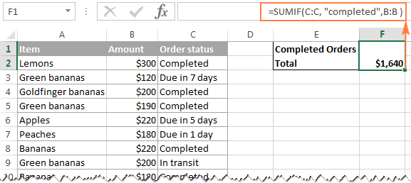
To calculate a conditional sum with multiple criteria, use the SUMIFS function. In the above example, to get the total of «Completed» orders with the amount over $200, use the following SUMIFS formula:
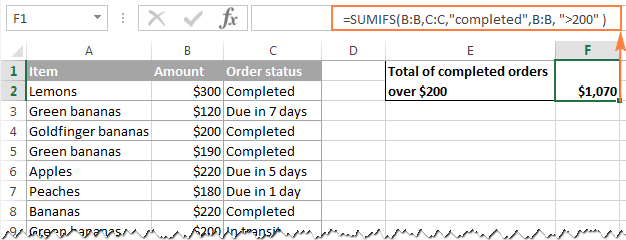
You can find the detailed explanation of the SUMIF and SUMIFS syntax and plenty more formula examples in these tutorials:
Note. The Conditional Sum functions are available in Excel versions beginning with Excel 2003 (more precisely, SUMIF was introduced in Excel 2003, while SUMIFS only in Excel 2007). If someone still uses an earlier Excel version, you’d need to make an array SUM formula as demonstrated in Using Excel SUM in array formulas to conditionally sum cells.
Excel SUM not working — reasons and solutions
Are you trying to add a few values or total a column in your Excel sheet, but a simple SUM formula doesn’t compute? Well, if the Excel SUM function is not working, it’s most likely because of the following reasons.
1. #Name error appears instead of the expected result
It’s the easiest error to fix. In 99 out of 100 cases, the #Name error indicates that the SUM function is misspelled.
2. Some numbers are not added
Another common reason for a Sum formula (or Excel AutoSum) not working are numbers formatted as text values. At first sight, they look like normal numbers, but Microsoft Excel perceives them as text strings and leaves them out of calculations.
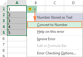
One of the visual indicators of text-numbers are the default left alignment and green triangles in top-left corner of the cells, like in the right-hand sheet in the below screenshot:
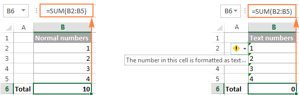
To fix this, select all problematic cells, click the warning sign, and then click Convert to Number.
If against all expectations that does not work, try other solutions described in: How to fix numbers formatted as text.
3. Excel SUM function returns 0
Apart from numbers formatted as text, a circular reference is a common source of problem in Sum formulas, especially when you are trying to total a column in Excel. So, if your numbers are formatted as numbers, but your Excel Sum formula still returns zero, trace and fix the circular references in your sheet (Formula tab > Error Checking > Circular Reference). For the detailed instructions, please see How to find a circular reference in Excel.
4. Excel Sum formula returns a higher number than expected
If against all expectations your Sum formula returns a bigger number than it should, remember that the SUM function in Excel adds both visible and invisible (hidden) cells. In this case, use the Subtotal function instead, as demonstrated in How to sum only visible cells in Excel.
5. Excel SUM formula not updating
When a SUM formula in Excel continues to show the old total even after you’ve updated the values in the dependent cells, most likely Calculation Mode is set to Manual. To fix this, go to the Formulas tab, click the dropdown arrow next to Calculate Options, and click Automatic.
Well, these are the most common reasons for SUM not working in Excel. If none of the above is your case, check out other possible reasons and solutions: Excel formulas not working, not updating, not calculating.
This is how you use a SUM function in Excel. I thank you for reading and hope to see you on our blog next week!
Practice workbook for download
You may also be interested in
Table of contents
how to use subtotal formula with multiple criteria when data was filtered?
Hello!
The answer to your question can be found in this article: Excel SUBTOTAL function with formula examples.
my data is in column wise and i want datewise total sum of «RECV» values .
Hi!
To calculate the sum of values by date, use the SUMIF function. See here for detailed instructions and examples.
I cannot get Autosum to return an answer when I sum up cells in the same row. I simply see the formula appear but not the answer.
go to formula bar than click show formula.
Hi
I use this formula to hide zero =IF(SUM(E7:P7)=0,»»,SUM(E7:P7)). In another cell when I want to subtract some value from this zero hide formula cell it results in #value! please give me the formula to get rid of the error value, hope will get it soon. Thanks in advance
Hello!
To avoid calculation problems, do not replace zero with an empty cell or space. Use a custom number format as described in this tutorial: Display zeroes as dashes or blanks. I hope my advice will help you solve your task.
I want to be able to find the top 10 results in a row list. I have the names in column A, then after each competition i have a column with the score and then points awarded. I have 15 competitions each with a score and points. I want to total the best 10 results for each person from the total of the points and exclude the score. I was using sumproduct but that needs a range, how do i get the total of the 10 best points?
Hello!
If I understand your task correctly, the following tutorial should help: LARGE IF formula in Excel: find highest values with criteria. If they don’t work for you, then please describe your task in detail, I’ll try to suggest a solution.
Hi
Thanks for the reply.
I have a list of names in column A, next to them i have a column in column b of scores, then in column c i have points. This is repeated in the rest of the columns so i have 15 sets of scores and points. My objective is to total the 10 best number of points per person and then sort the list on this total.
Name Score Points Score Points Score Points Total(this example best 2 points)
Woods 78 5 36 15 81 10 25
Storey 81 5 40 20 76 15 35
Hi!
Give an example of the result you want to get.
Hello: Need some help here
I have below and based on title, I need to get the total salary for admins or any title based condition?
TITLE SALARY TITLE SALARY
ADMIN 200 ADMIN 180
ANALYST 100 PROGRAMMER 125
Programmer 100 ANALYST 130
Hello!
To get the sum based on a condition, use the SUMIF function. I recommend reading this guide: How to use SUMIF function in Excel with formula examples.
I have a Table. Lets say in the table there in data in column B say rows 3-10. Out side of the table I have a sum formula that sums up rows 3-10. When I add another line to the table my sum formula should sum up rows 3-11 but it only does row 3-10
Hi!
Convert your data to an Excel table. Then when you add data to the table, the formulas will automatically change.
i have a formula to add selected cells in a row =SUM(G47:H47:AI47:AJ:47:AL47:AN47) but it is giving me the sum of all cells between G47 and AN47, why? and how can i fix this? it used to work fine, now it doesn’t. What changed?
I found the problem, you need to enter a comma between the cells in the formula not a colon.
Amazing content.. helped a lot !
Thank you ! The conditional sum is exactly what I was looking for !
I’ve been trying to format my sheet to keep track of loan given to employees, with conditional summation (i.e at last column with ticked box) and to keep testing if employee loan balance is zero. Kindly help. Link is shared below. Thanks in advance. Kindly use the tab tagged «B».
My requirement is auto sl. number under filtering data . if any sl. no. of row is invisible which to be auto numbered with next visible raw . Is it possible to formulated my requirement. As example if i invisible the raw no. 2. by Filtered data.
Sl. No. Vendor Code Company Code Vendor Name City
1 10001784 2100 Mt Bashundhara Lpg-3 Dhaka
2 10003438 2100 MT. Bashundhara LPG 6 Umme Kulsum Road,Bashundhara R/A
3 10003484 2100 M. T. Bashundhara LPG-01 Pangaon, Konda, South Keranigonj,Dh
4 50003794 2100 MT. Bashundhara LPG 2 Dhaka
5 60000018 2100 M. T. BASHUNDHARA LPG-04 Dhaka
6 60000019 2100 M. T. Bashundhara LPG-05 Dhaka
Thanks, it works
Thanks for the comprehensive answer to how to sum only visible cells. Very helpful.
Thank you 4 gr8 infos
Please help me,To find the automatically sum amount of particular raw if i colored raw.for example i prepared chart of receivable amount.when i received money i just shide the color on who gave money.i want to know how to make a formula to avoid the colored raw.please help me
define for me the following terms used in spreadsheet
Function
An operator
am appreciative for all your services
D/Sir
To find the Total I am using the formula subtotal(109,M10:U10) but the result is adding the hidden columns also.Any solution to this problem?
Thanks
Sudip C. Pal
Question 1: Can someone help me understand how this formula works
A1:1
A2:2
A2:3
=Sum(A1:A3-1)= 2 ## Need help with this Question?
Question 2:
A1 B1 C1
=Sum(A1:C1)-Sum(A1-1:C1-1) ## this Formula is not working, any comments?
answer to Question 1:
SUM(A1:A3-1) subtracts 1 from the value of each cell within specified range (A1 to A3), then adds the resultants.
(1-1)+(2-1)+(3-1)=0+1+2=3
answer to Question 2:
SUM(A1-1:C1-1) generates an error.
In a file, i maintain 2 sheet summary and detail. Detail sheet is datewise and summary sheet is tank no wise, so i did filter in detail sheet and in summary sheet i used formula of subtotal(9,(range)) for calculating total amount against particular tanker. But when i remove filter, total of summary sheet gets changed. So please let me know which formula I have to used.
Thanks.
today i enter the value in column B5 and the total of column B5=c55, next day i enter the value in column b5, then it must added automatically in column C5 automatically
Thanks. It helped me a lot.
the auto sum for visible data (not hidden) only instructions do not work
I have to find the cgpa of my class result. i have done summing up amd grading in excel sheet. but cant find out the formula
Too much thanks, It’s very useful.
Hi,
How do I sum visable cells only(filtered)
VISIBLE CELLS POPULATE A ROW
COLUMN (FILTERED)
C G H K L N
ROW. 6 3 5 9 2 4 = SUM ?
I have a problem to sum only the digits which cells are formatted by kg, like
5 kgs
4 yds
3 kgs
2 kgs
7 yds
_______________
I would like get sum result only with the kgs, above result should be 10 kgs.
Could you pls advise how to solve it.
It can be done pretty simply if you split the text from the numbers like this:
Where the numbers are in A29:A33 and the text is in B29:B33 the formula is:
=SUMIF(B29:B33,»*kgs*»,A29:A33)
How to find the sum of formula cells only ?
My problem is viewing:
If I enter amounts with decimals or cents I am not able to view the whole total (the amounts to the right of the decimal point). How do I extend the area to view the entire total?
I am trying to sum columns and if the total is 40or more, change the total to 40 which is the set up maximum. And if the total is less than 40, then just show the correct total. Can somebody help me with the formula? Thank you.
If I understand your task correctly, please try the following formula:
Hope this will help you!
I would appreciate if someone could help. I have an excel document that is exported from simply. It has a column with subtotals (=SUBTOTAL(9,H12:H17))for each property and I would like to total the subtotals without having to do in manually.(c5+c17+c27) Thank you in advance
Hello everyone,Challanging question for me (Please understand the issue carefully before answering hapazardly)
C1:C10 (weight gain)= 1,2,3,4,5,6,7,8,9,10
A1:A10 Age of child in month) = 11,20,23,40,55,60,32,80,90,95,160
Now I make class interval in B1:B6 as (0-1)(2-6)(7-12)(13-24)(25-60)(61-168) for A1:A10
I did: sum age of child meeting (0-1) in B1 which is always showing 0 gram weight increase, for those child who doesnot exist (mistake calculation), want to display empty cell for such case and sum only of there is value in column B. Formulas working fine for the existing child.
I couldnot localize how to calculate for those rows that donot exist in A and display empty cells in B.
Again, for reminder: excel is showing 0 gram increase for those child that doesnot exist in my excel sheet.
I tried 100s of formulas but non of them worked.
Please suggest same formula for all calculating in all class intervals as mentioned above
Hello everyone,Challanging question for you all (Please understand the issue carefully before answering hapazardly)
C1:C10 (weight gain)= 1,2,3,4,5,6,7,8,9,10
A1:A10 Age of child in month) = 11,20,23,40,55,60,32,80,90,95,160
Now I make class interval in B1:B10 as (0-1)(2-6)(7-12)(13-24)(25-60)(61-168) for A1:A10
I did: sum age of child meeting (0-1) in B1 which is always showing 0 gram weight increase, for those child who doesnot exist (mistake calculation), want to display empty cell for such case and sum only of there is value in column J. Formulas working fine for the existing child.
I couldnot localize how to calculate for those rows that donot exist in A and display empty cells in B.
Again, for reminder: excel is showing 0 gram increase for those child that doesnot exist in my excel sheet.
I tried 100s of formulas but non of them worked.
Please suggest same formula for all calculating in all class intervals as mentioned above
Please solved this example : —
Analyze Data Actual Default
A 486 53
B 150
C 10
Total
how to calculate total without sum function or + operator
how to compute (G7x5)+(H7x4)in a horizontal row
how to calculate the sum of the following?
(G7X5)+(H7X4)+(I7X3)+(J7X2)+(K7X1)
Please enlighten me..Thanks in advance.
Ram 2000
Raj 400
Pop 221
Arun 339
sohan 3382
I want to calculate the total of all.. but skip «pop» and «ram» automatically.
Eg:
Ram 2000
Raj 400
Pop 221
Arun 339
sohan 3382
the total of this will be «6342.» but it automatically skip pop & ram & give answer «7721.»
it is very well. i cleared all my doubts. but how i can iget ablebits in my windows 10 computer
I want to total all all rows in Column A minus Column B row1,2,3. sum into Column C row 1,2,3. need a formula please
Hello, Paul,
try using the following:
=SUM(A:A)-SUM(B1:B3)+SUM(C1:C3)
I want to total all all rows in Column A minus Column row1,2,3. sum into Column C row 1,2,3. need a formula please
i have small doubt in excel pl solve this. details given below
i have on table some rows and columns
sl.no. amend no. scope qty amt
1 1 1234 1500 1000.00
2 2 1234 50 800.00
3 1 324 100 200.00
4 1 545 10 50.00
6 2 324 87 65.00
7 3 324 54 85.00
Now i want like every scope highest amend no details.
pl help me
I have a budget worksheet by month. Totaled income/expense at the end of each month. Jan=column B etc. but when adding income/expense to Feb (column C) is adds or remove from my January total.
My formula for January is =SUM(B62-B49)so why is adding to column C effecting this?
I want to run an inventory sheet where I can take from a beginning number or add to that same number and have it give me a quantity on hand. Example. I have 20 of something and tomorrow I remove 4 of them so I need a box to calculate that I now have 16 but the next day I add 10 back into the qty- I now want that box to show I have 26.
I want to know i have excel sheet i want to fix the SUM formula after filter the sheet in some selected row actually i have tried after filter but which cell is hide that cell Qty also adding in total please check tell me if you have any formula.
inplace of c2:c6 substitute the column and row details as per your worksheet
hello, I have another doubt in which i was able to add filted numbers but when i open the unfiltered sheet it goes back to sum of all the numbers. please help.
i filtered the items to make a total of different items but when i change the filter to «all» it changes to sum of all the numbers in the range.
lots of good stuff herein — thanks!
But, I want to make bold the «sum» product of auto-summing in the bottom bar of the Excel screen (where «sum» is accompanied by «average» and «count»).
Can this be accomplished?
I’m 85 and even with glasses the sum product is not very visible. Microsoft should change this and make it bold. All octogenarians would give a shout-out if they did.
actually i have approximately 25 row in that i want to sum like this way
1row +3rd row + 5th row + 7th row . if there is any formula please provide me
How to sum a whole row
To sum the entire row with an indefinite number of columns, supply a whole-row reference to your Excel Sum formula, e.g.:
Please remember that you shouldn’t enter that ‘Sum of a row’ formula in any cell of the same row to avoid creating a circular reference because this would result in a wrong calculation, if any:
mam please elaborate this with xls file i am not able to understand it
How add if table like 24kg
25 kg
What is the formula to sum up a total billing per Customer# by Customer name. I also need a formula of average billing and the highest billing per Customer.
Example:
Column A B C D E F
Customer# Customer Name Bill Amt Total Pd Amt Avg Bill HighestBill YTD
1 A $125 $125
1 A $0 $0
2 B $85 $85
2 B $225 $225
3 C $35 $35
3 C $67 $67
4 D $324 $324
4 D $455 $455
4 D $124 $124
4 D $0 $0
I need the SUMIF formula if applicable. Thank you for your help.
This formula is good but can I replace row number for customer name? =IF(AND($B2 Reply
What is the formula to sum up a total billing per Customer# by Customer name. I also need a formula of average billing and the highest billing per Customer.
Example:
Column A B C D E F
Customer# Customer Name Bill Amt Total Pd Amt Avg Bill Total Amt YTD
1 A $125 $125
1 A $0 $0
2 B $85 $85
2 B $225 $225
3 C $35 $35
3 C $67 $67
4 D $324 $324
4 D $455 $455
4 D $124 $124
4 D $0 $0
I need the SUMIF formula if applicable. Thank you for your help.
ms office is the heart of computer programing
I’m a new user I have a units and and unit cost say I have 50 units and each are 1.99 how do I get home he sum.I would really appreciate it.
Setting up a work sheet I want to use only 4 columns: A=Date B=Invoice # (ie 2012000) C= amount ie (345.00) D=running total of column C of each entry as applied or entered
Also is a column header needed for each column?
I have a data table that is updated daily, for example, a new column is added daily, I want to find the difference between the last updated column & first column. But, don’t want to rewrite formula each time.
Can you help me.
thanks for the tip on How to sum only filtered.
Источник
To sum a range of cells, use the SUM function. To sum cells based on one criteria (for example, greater than 9), use the following SUMIF function (two arguments). To sum cells based on one criteria (for example, green), use the following SUMIF function (three arguments, last argument is the range to sum).
How do you total a row in Excel?
You can quickly total data in an Excel table by enabling the Toggle Total Row option.
- Click anywhere inside the table.
- Click the Table Design tab > Style Options > Total Row. The Total row is inserted at the bottom of your table.
What is the formula for SUM in Excel?
The SUM function adds values. You can add individual values, cell references or ranges or a mix of all three. For example: =SUM(A2:A10) Adds the values in cells A2:10.
How do I apply a formula to an entire column in Excel?
The easiest way to apply a formula to the entire column in all adjacent cells is by double-clicking the fill handle by selecting the formula cell. In this example, we need to select the cell F2 and double click on the bottom right corner. Excel applies the same formula to all the adjacent cells in the entire column F.
How do I enable filtering?
Try it!
- Select any cell within the range.
- Select Data > Filter.
- Select the column header arrow .
- Select Text Filters or Number Filters, and then select a comparison, like Between.
- Enter the filter criteria and select OK.
Why is Excel not showing sum?
The most common reason for AutoSum not working in Excel is numbers formatted as text. … To fix such text-numbers, select all problematic cells, click the warning sign, and then click Convert to Number.
How do you fill down in Excel using keyboard?
Simply do the following:
- Select the cell with the formula and the adjacent cells you want to fill.
- Click Home > Fill, and choose either Down, Right, Up, or Left. Keyboard shortcut: You can also press Ctrl+D to fill the formula down in a column, or Ctrl+R to fill the formula to the right in a row.
How do I do a percentage formula in Excel?
The percentage formula in Excel is = Numerator/Denominator (used without multiplication by 100). To convert the output to a percentage, either press “Ctrl+Shift+%” or click “%” on the Home tab’s “number” group.
How do I AutoFill in Excel using keyboard?
Alt + E+I+S then press ENTER. By Default, Linear option is selected, that’s for numeric values ! For auto-filling months or days, select Autofill option and then ENTER. Use Ctlr+Down/Right key to select the cells you want to fill and press Ctrl+D (to fill down) or Ctrl+R (to fill right).
How do you AutoFill in Excel without dragging?
Alternatively, press hit Ctrl + D to fill down or Ctrl + R to fill right. Both shortcuts give the same result. Now the formula is copied to the whole column without dragging the fill handle.
How do I fill the same data in Excel?
Insert the same data into multiple cells using Ctrl+Enter
- Select all the blank cells in a column.
- Press F2 to edit the last selected cell and type some data: it can be text, a number, or a formula (e.g. “_unknown_”)
- Press Ctrl+Enter instead of Enter. All the selected cells will be filled with the data that you typed.
How do I fill the same cell value in Excel?
Place the cursor in the bottom right corner of the cell you just typed in until you see a plus sign. With the left mouse button, press and drag the Fill Handle (plus sign) to highlight all of the cells you want filled. Release the mouse button and the cells are filled with the value typed in the first cell.
Where is AutoFill in Excel?
The Fill button is located in the Editing group right below the AutoSum button (the one with the Greek sigma). When you select the Series option, Excel opens the Series dialog box. Click the AutoFill option button in the Type column followed by the OK button in the Series dialog box.
How do I AutoFill large data in Excel?
Why does AutoFill not work in Excel?
In case you need to get Excel AutoFill not working, you can switch it off by doing the following: Click on File in Excel 2010-2013 or on the Office button in version 2007. Go to Options –> Advanced and untick the checkbox Enable fill handle and cell drag-and-drop.
What is AutoFill in Excel with example?
What is AutoFill? Excel has a feature that helps you automatically enter data. If you are entering a predictable series (e.g. 1, 2, 3…; days of the week; hours of the day) you can use the AutoFill command to automatically extend the sequence.
How do I AutoFill in Excel Mobile?
How is AutoFill method is useful?
AutoFill is a very useful Excel feature. It allows you to create entire columns or rows of data which are based on the values from other cells. In other words, Excel compares the selected data and tries to guess the next values that will be inserted.
How do I autofill dates in Excel?
Key in the starting date and format the cell. Hover the mouse over the lower right edge of the cell until you see the Fill Handle. With the RIGHT mouse button pressed, drag to select the cells to autofill. Release the mouse button and select either Fill Months or Fill Years from the menu that displays.
What is the fill handle in Excel?
The active cell on an Excel worksheet has a small square on its lower-right corner. That square is called the fill handle. You can use that fill handle to copy and paste the cell’s data in any direction. Just put your mouse pointer over the fill handle, press the mouse button, and drag down, right, left, or up.
How do you autofill in sheets?
Use autofill to complete a series
- On your computer, open a spreadsheet in Google Sheets.
- In a column or row, enter text, numbers, or dates in at least two cells next to each other.
- Highlight the cells. You’ll see a small blue box in the lower right corner.
- Drag the blue box any number of cells down or across.
How do I autofill dates in Excel on IPAD?
How do you put a formula in Excel on a touch screen phone?
Tap a cell. Tap, then drag the selection handler. Tap on a cell, and then flick the selection handle in the direction you want to select. Tap in the formula bar.
How do I access Google autofill?
Tap the three dots — located either to the right of the address bar (on Android) or the bottom-left corner of the screen (on iPhone) — and select “Settings.” 2. To change your settings for autofill addresses, tap “Addresses and more” and toggle the feature on or off, or edit your saved information as necessary. 3.
Where is auto fill on Google Sheets?
Excel Column Total (Table of Contents)
- Definition of Excel Column Total
- Examples of Excel Column Total
Definition of Excel Column Total
In excel there are various methods to know the total of numbers inside a column, in this article we will discuss those methods and shortcuts that how do we identify the total sum of numbers in a column. First, we should understand what is the basic definition of Excel Column Total we are talking about. Column Total means the sum of the numbers present inside a column. Now let us go through with various examples on how we can get Totals of Columns in Excel.
Examples of Excel Column Total
Let us discuss examples of Excel Column Total.
You can download this Column Total Excel Template here – Column Total Excel Template
Example #1
Let us begin with the most basic method to know the total of numbers in a column. In this method, we will select a column to see what is the total of the column.
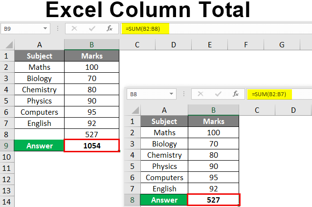
1. Let us make a table of data in sheet 1 as shown below:
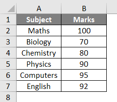
2. Now select whole column B as shown in the image below:

3. In bottom right corner we can see on the status bar that excel automatically calculates the total of the column for us. Refer below screenshot for the preview,
![]()
This status bar excel shows us what is the total of column B as Sum which is 527.
Example #2
For example one we have seen how excel has given us total by selecting the total column. But what will happen if we select only the data range in the column rather than the entire column. Let us find out in this example,
1. Let us use the same data from sheet 1 for this example too.
2. Instead of selecting the entire column as we did in example 1, we will select only the data range as shown in below image:
3. Now in the same status bar in the bottom right corner let us check the total as result, it will be same as we have seen in example 1,
![]()
So even we select the data range in the column or we select the entire column we will get the same total as result.
Note: Now there is a catch for both example 1 and example 2 that these totals in the columns are temporary means the total can change as soon as the data will change, in the column for example till B7 we had data in the column and if we increase data in B8 the total will increase.
Example #3
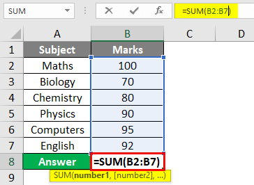
In the above examples, we have seen that how excel calculates temporary total in the status bar, however, there are some inbuilt formulas through which a user can calculate the total of the columns in excel by himself, one of such formulas is known as Auto Sum function. It is an inbuilt function in excel which calculates the sum of the numbers of the given data range. There is a keyboard shortcut to use the Auto Sum function in excel which is ‘ALT” + “=” buttons.
1. Now let us copy the same data from sheet 1 to sheet 2 for our data table as shown below:
2. In B8 cell let us press the keyboard shortcut we talked about above and see the result as follows:
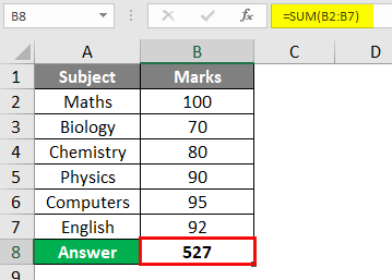
3. Excel will automatically compute the sum from the data range in the given column, when we press Enter we will get the result as follows:
Example #4
Apart from Auto Sum in Excel which is initiated by a keyboard shortcut, there is an inbuilt sum function in excel which allows us to select specific cells in any columns in excel to compute sum in the columns. Let us use the sum function in this example.
1. In the same data table in cell B9 enter the following formula as shown below:
2. Press “Tab” button from keyboard for the sum function and select the data range from the table as shown in the below image:
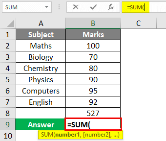
3. When we press Enter we will see the result of the sum of the numbers from B2 to B8, remember that in cell B8 we already have the sum of the numbers from B2 to B7.
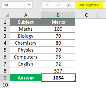
Explanation of Excel Column Total
In any worksheet of excel data is present in both rows and columns in form of cells. Each individual cells contain data, when these cells contain numbers excel automatically gives us certain features to calculate the total of these numbers by different methods. Some of the methods are inbuilt which is a feature of excel but they give us temporary result, while the formulas which are used to calculate the total of the numbers give us permanent results.
How to Use Excel Column Total?
As we have discussed in the above examples we have seen that there are four methods to calculate Excel Column Total and they are as follows:
- First is by selecting the entire column.
- The second method is by selecting the data range in the column.
- In the third method, we had used the Auto sum function to calculate the total.
- The best procedure to calculate the total is by using the sum function.
Things to Remember
There are few things to remember about Excel Column Total and they are as follows,
- Column Total Means the sum of numbers in a given column.
- When we select a column for column total it ignores the header and calculates the sum of the numbers in a given column.
- Auto Sum function only calculates the sum from the data range above the function.
- By using Sum function we can select certain cells for which we want the total in the column.
Recommended Articles
This has been a guide to Excel Column Total. Here we discuss How to Excel Column Total along with practical examples and a downloadable excel template. You can also go through our other suggested articles –
- Column Header in Excel
- Freeze Columns in Excel
- COLUMNS Formula in Excel
- Moving Columns in Excel
You’re likely going to come across the need for running totals if you’re dealing with any sort of daily data.
Imagine you track sales each day. Your data contains a row for each date with a total sales amount, but maybe you want to know the total sales for the month at each day. This is a running total, it’s the sum of all sales up to and including the current days sales.
In this post we’ll cover multiple ways to calculate a running total for your daily data. We’ll explore how to use worksheet formulas, pivot tables, power pivot with DAX and power query.
We’ll also explore what happens to the running total calculation when inserting or deleting rows of data and how to update the results.
Get the file with all the examples.
Running Totals with a Simple Formula
It’s possible to create a basic running total formula using the + operator.
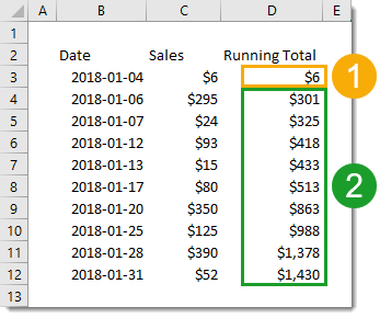
However, we’ll need to use two different formulas to get the job done.
- =C3 will be the first formula and will only be in the first row of the running total.
- =C4+D3 will be in the second row and can be copied down the remaining rows for the running total.
The formula in our first row can’t add the cell above it to the total as it contains a text value for a column heading. This would cause a #VALUE! error to appear in the running total since the + can’t handle text values. We avoid this with a different formula in the first row which doesn’t reference the cell above.
What happens to the running total when we insert or delete rows in our data?
Inserting a new row will result in a gap in the running total. To fix this, we’ll need to copy the formula down from the first cell above the newly inserted rows all the way down to the last row.
Deleting any rows will result in #REF! errors since deleting a row means deleting a cell referenced by the formula below it. To fix this, we’ll need to copy the formula down from the last error-free cell all the way down to the last row.
Running Totals with a SUM Formula
We can avoid the awkwardness of using two different formulas in our running total column by utilizing the SUM function instead of the + operator. When the SUM function encounters a text cell it will treat it the same as a though it contained a 0.
This way we can use the following formula uniformly for every row including the first row.
=SUM(C3,D2)
This formula will reference the column heading containing text for the first row, but this ok as it’s treated like a 0.
When inserting or deleting rows, we will still encounter the same problems with blank cells and errors. We can fix them the same way as with running totals in the simple formula method.
Running Totals with a Partially Fixed Range
Another option with the SUM function is to only reference the Sales column and use a partially fixed range reference.
If we use the following formula =SUM($C$3:C3), we can copy and paste this down the range. It won’t reference any column headings and the range referenced will grow to each row.
Unfortunately, this too will have the same problems (and solutions) with inserting or deleting rows.
Running Totals with a Relative Named Range
We can avoid the problems with inserting and deleting rows from our data if we use a relative named range. This will refer to the cell directly above no matter how many rows we insert or delete.
This is a trick that involves temporarily switching the Excel reference style from A1 to R1C1. Then defining a named range using the R1C1 notation. Then switching the reference style back to A1.
In R1C1 reference style, cells are referred to by how far away they are from the cell using the reference. For example, =R[-2]C[3] refers to the cell 2 up and 3 to the right of the cell using this formula.
We can use this relative referencing to create a named range that’s always one cell above the referring cell with the formula =R[-1]C.
To switch reference style, go to the File tab then choose Options. Go to the Formula section in the Excel Options menu and check the R1C1 reference style box and then press the OK button.
Now we can add our named range. Go to the Formula tab of the Excel ribbon and choose the Define Name command.
Insert a name like “Above” as the name of the range. Add the formula =R[-1]C into the Refers to input and press the OK button.
We can now switch Excel back to the default reference style. Go to the File tab > Options the Formula section > uncheck the R1C1 reference style box > then press the OK button.
Now we can use the formula =SUM([@Sales],Above) in our running total column.
The named range Above will always refer to the cell directly above. When we insert or delete rows, the relative named range will adjust accordingly and no action is needed.
In fact if we place our data in an Excel Table then the formula will automatically fill down for any new rows since the formula is uniform for the entire column. No action is needed to copy down any formulas.
Running Totals with a Pivot Table
Pivot tables are super useful for summarizing any type of data. There’s more to them than just adding, counting and finding averages. There are many other types of calculations built in, and there is actually a running total calculation!
First, we need to insert a pivot table based on the data. Select a cell inside the data and go to the Insert tab and choose the PivotTable command. Then go through the Create PivotTable window to choose where you want the pivot table, either in a new worksheet or somewhere in an existing one.
Add the Date field into the Rows area of the pivot table, then add the Sales field into the Values area of the pivot table. Now add another instance of the Sales field into the Rows area.
We should now have two identical Sales fields with one of them being labelled Sum of Sales2. We can rename this label anytime by simply typing over it with something like Running Total.
Right click on any of the values in the Sum of Sales2 field and select Show Value As then choose Running Total In.
We want to show the running total by date, so in the next window we need to select Date as the Base Field.
That’s it, we now have a new calculation which displays the running total of our sales inside the pivot table.
What happens if we add or delete a row in our source data, how does this affect the running total? The pivot table calculations are dynamic and will take any new data into account in its running total calculation, we will just need to refresh the pivot table.
Right click anywhere inside the pivot table and choose Refresh from the menu.
Running Totals with Power Pivot and DAX Measures
The first couple steps for this are the exact same using a regular pivot table.
Select a cell inside the data and go to the Insert tab and choose the PivotTable command.
When you come to the Create PivotTable menu, check the Add this data to the Data Model box to add the data to the data model and enable it for use with power pivot.
Place the Date field in the Rows area and the Sales field in the Values area of the pivot table.
With power pivot, we will need to create any extra calculations we want using the DAX language. Right click on the table name in the PivotTable Fields window, then select Add Measure to create a new calculation. Note, this is only available with the data model.
=CALCULATE (
    SUM ( Sales[Sales] ),
    FILTER (
        ALL (Sales[Date] ),
        Sales[Date] <= MAX (Sales[Date])
    )
)
Now we can create our new running total measure.
- In the Measure window, we need to add a Measure Name. In this case we can name the new measure as Running Total.
- We also need to add the above formula into the Formula box.
- The cool thing about power pivot is the ability to assign a number format to a measure. We can choose the Currency format for our measure. Whenever we use this measure in a pivot table the format will automatically be applied.
Press the OK button and the new measure will be created.
There will be a new field listed in the PivotTable Fields window. It has a small fx icon on the left to denote that it’s a measure and not a regular field in the data.
We can use this new field just like any other field and drag it into the Values area to add our running total calculation into the pivot table.
What happens to the running total when we add or remove data from the source table? Just like a regular pivot table, we simply need to right click on the pivot table and select Refresh to update the calculation.
Running Totals with a Power Query
We can also add running totals to our data using power query.
First we need to import the table into power query. Select the table of data and go to the Data tab and choose the From Table/Range option. This will open the power query editor.
Next we can sort our data by date. This is an optional step we can add so that if we change the order of our source data, the running total will still appear by date.
Click on the filter toggle in the date column heading and choose Sort Ascending from the options.
We need to add an index column. This will be used in the running total calculation later on. Go to the Add Column tab and click on the small arrow next to the Index Column to insert an index starting at 1 in the first row.
We need to add a new column to our query to calculate the running total. Go to the Add Column tab and choose the Custom Column command.
We can name the column as Running Total and add the following formula.
List.Sum(List.Range(#"Added Index"[Sales],0,[Index]))
The List.Range function creates a list of values from the Sales column starting at the 1st row (0th item) which spans a number of rows based on the value in the index column.
The List.Sum function then adds up this list of values which is our running total.
We no longer need the index column, it has served its purpose and we can remove it. Right click on the column heading and select Remove from the options.
We’ve got our running total and are finished with the query editor. We can close the query and load the results into a new worksheet. Go to the Home tab of the query editor and press the Close & Load button.
What happens with the running total when we add or remove rows from our source data? We will need to refresh the power query output table to update the running total with the changes. Right click anywhere on the table and choose Refresh to update the table.
With the optional sorting step above, if we add dates out of order to the source data, power query will sort by date and return the correct order by date for the running total.
Conclusions
There are many different options for calculating running totals in Excel.
We’ve explored options including formulas in the worksheet, pivot tables, power pivot DAX formulas, and power query. Some offer a more robust solution when adding or removing rows from the data, other methods offer an easier implementation.
Simple formulas in the worksheet are easy to set up but won’t handle inserting or deleting new rows of data easily. Other solutions like pivot tables, DAX and power query are more robust and handle inserting or deleting rows of data easily but are harder to set up.
It’s good to be aware of the pros and cons of each method and choose the one best suited. If you won’t be inserting or deleting new data, then worksheet formulas might be the way to go.
About the Author
John is a Microsoft MVP and qualified actuary with over 15 years of experience. He has worked in a variety of industries, including insurance, ad tech, and most recently Power Platform consulting. He is a keen problem solver and has a passion for using technology to make businesses more efficient.