
SUM function
The SUM function adds values. You can add individual values, cell references or ranges or a mix of all three.
For example:
-
=SUM(A2:A10) Adds the values in cells A2:10.
-
=SUM(A2:A10, C2:C10) Adds the values in cells A2:10, as well as cells C2:C10.

SUM(number1,[number2],…)
|
Argument name |
Description |
|---|---|
|
number1 Required |
The first number you want to add. The number can be like 4, a cell reference like B6, or a cell range like B2:B8. |
|
number2-255 Optional |
This is the second number you want to add. You can specify up to 255 numbers in this way. |
This section will discuss some best practices for working with the SUM function. Much of this can be applied to working with other functions as well.
The =1+2 or =A+B Method – While you can enter =1+2+3 or =A1+B1+C2 and get fully accurate results, these methods are error prone for several reasons:
-
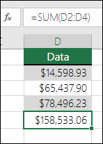
Typos – Imagine trying to enter more and/or much larger values like this:
-
=14598.93+65437.90+78496.23
Then try to validate that your entries are correct. It’s much easier to put these values in individual cells and use a SUM formula. In addition, you can format the values when they’re in cells, making them much more readable then when they’re in a formula.

-
-
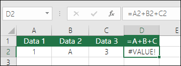
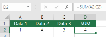
#VALUE! errors from referencing text instead of numbers
If you use a formula like:
-
=A1+B1+C1 or =A1+A2+A3
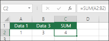
Your formula can break if there are any non-numeric (text) values in the referenced cells, which will return a #VALUE! error. SUM will ignore text values and give you the sum of just the numeric values.
-
-
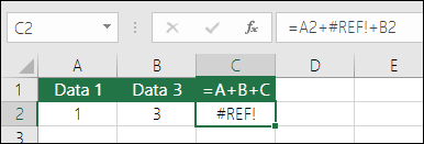
#REF! error from deleting rows or columns
If you delete a row or column, the formula will not update to exclude the deleted row and it will return a #REF! error, where a SUM function will automatically update.
-
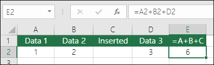
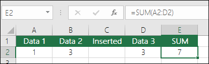
Formulas won’t update references when inserting rows or columns
If you insert a row or column, the formula will not update to include the added row, where a SUM function will automatically update (as long as you’re not outside of the range referenced in the formula). This is especially important if you expect your formula to update and it doesn’t, as it will leave you with incomplete results that you might not catch.
-
SUM with individual Cell References vs. Ranges
Using a formula like:
-
=SUM(A1,A2,A3,B1,B2,B3)
Is equally error prone when inserting or deleting rows within the referenced range for the same reasons. It’s much better to use individual ranges, like:
-
=SUM(A1:A3,B1:B3)
Which will update when adding or deleting rows.
-
-
I just want to Add/Subtract/Multiply/Divide numbers See this video series on Basic Math in Excel, or Use Excel as your calculator.
-
How do I show more/less decimal places? You can change your number format. Select the cell or range in question and use Ctrl+1 to bring up the Format Cells Dialog, then click the Number tab and select the format you want, making sure to indicate the number of decimal places you want.
-
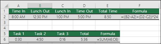
How do I add or subtract Times? You can add and subtract times in a few different ways. For example, to get the difference between 8:00 AM — 12:00 PM for payroll purposes you would use: =(«12:00 PM»-«8:00 AM»)*24, taking the end time minus the start time. Note that Excel calculates times as a fraction of a day, so you need to multiply by 24 to get the total hours. In the first example we’re using =((B2-A2)+(D2-C2))*24 to get the sum of hours from start to finish, less a lunch break (8.50 hours total).
If you’re simply adding hours and minutes and want to display that way, then you can sum and don’t need to multiply by 24, so in the second example we’re using =SUM(A6:C6) since we just need the total number of hours and minutes for assigned tasks (5:36, or 5 hours, 36 minutes).
For more information, see: Add or subtract time.
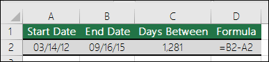
-
How do I get the difference between dates? As with times, you can add and subtract dates. Here’s a very common example of counting the number of days between two dates. It’s as simple as =B2-A2. The key to working with both Dates and Times is that you start with the End Date/Time and subtract the Start Date/Time.
For more ways to work with dates see: Calculate the difference between two dates.
-
How do I sum just visible cells? Sometimes, when you manually hide rows or use AutoFilter to display only certain data you also only want to sum the visible cells. You can use the SUBTOTAL function. If you’re using a total row in an Excel table, any function you select from the Total drop-down will automatically be entered as a subtotal. See more about how to Total the data in an Excel table.
Need more help?
You can always ask an expert in the Excel Tech Community or get support in the Answers community.

See Also
Learn more about SUM
The SUMIF function adds only the values that meet a single criteria
The SUMIFS function adds only the values that meet multiple criteria
The COUNTIF function counts only the values that meet a single criteria
The COUNTIFS function counts only the values that meet multiple criteria
Overview of formulas in Excel
How to avoid broken formulas
Find and correct errors in formulas
Math & Trig functions
Excel functions (alphabetical)
Excel functions (by Category)
Need more help?
Want more options?
Explore subscription benefits, browse training courses, learn how to secure your device, and more.
Communities help you ask and answer questions, give feedback, and hear from experts with rich knowledge.
-
1
Определите какую колонку цифр или слов вы хотите сложить.
-
2
Выберите клетку для результата суммы.
-
3
Напишите знак равно и потом SUM. Вот так: =SUM
-
4
Напишите ссылку на первую клетку, потом двоеточие и ссылку на последнюю клетку. Вот так: =Sum(B4:B7).
-
5
Нажмите enter. Excel сложит номера в клетках B4 на B7
Реклама


-
1
Если у вас есть колонка с цифрами, используйте автосумму. Нажмите на клетку в конце списка, который вы хотите сложить (под цифрами).
- В Windows, нажмите Alt + = одновременно.
- На Mac, нажмите Command + Shift + T одновременно.
- Или на любом компьютере, вы можете нажать на кнопку Автосумма в меню/ленте Excel.
-
2
Убедитесь, что выделенные клетки – это те, которые вы хотите просуммировать.
-
3
Нажмите Enter для результата.
Реклама


-
1
Если у вас есть несколько колонок для сложения, наведите курсор на правую нижнюю часть клетки с результатом. Курсор изменит вид на крестик.
-
2
Удерживайте левую кнопки мышки и перетяните ее на клетки аналогичных колонок, сумму которых вы хотите получить.
-
3
Наведите мышку на последнюю клетку и отпустите. Excel автоматически заполнит результаты сумм выбранных колонок!
Реклама


Советы
- Как только вы начнете писать после знака =, Excel покажет выпадающий список доступных функций. Нажмите на функцию, которую хотите использовать, в нашем случае, на SUM.
- Представьте, что двоеточие – это слово НА, например, B4 НА B7.
Реклама
Об этой статье
Эту страницу просматривали 12 332 раза.
Была ли эта статья полезной?
Enter the SUM function manually to sum a column In Excel
- Click on the cell in your table where you want to see the total of the selected cells.
- Enter =sum( to this selected cell.
- Now select the range with the numbers you want to total and press Enter on your keyboard. Tip.
Contents
- 1 How do you write a sum formula in Excel?
- 2 How do I sum an entire column in Excel?
- 3 How do you do sum in Excel quickly?
- 4 What is the symbol for AutoSum in Excel?
- 5 How do you AutoSum in Excel 2010?
- 6 What is a sum example?
- 7 What is the sum of 13?
- 8 How do I SUM a column in Excel 2016?
- 9 How do you use plus in Excel?
- 10 What are the sums of 4?
- 11 Does sum add or subtract mean?
- 12 What does sum mean in a math equation?
- 13 What can make 11?
- 14 What are the sums of 14?
- 15 What is a sum of 14 and a difference of 6?
- 16 What is the sum of 18 and difference of two?
How do you write a sum formula in Excel?
Use AutoSum or press ALT + = to quickly sum a column or row of numbers.
- First, select the cell below the column of numbers (or next to the row of numbers) you want to sum.
- On the Home tab, in the Editing group, click AutoSum (or press ATL + =).
- Press Enter.
How do I sum an entire column in Excel?
To add up an entire column, enter the Sum Function: =sum( and then select the desired column either by clicking the column letter at the top of the screen or by using the arrow keys to navigate to the column and using the CTRL + SPACE shortcut to select the entire column. The formula will be in the form of =sum(A:A).
How do you do sum in Excel quickly?
The Autosum Excel shortcut is very simple – just type two keys:
- ALT =
- Step 1: place the cursor below the column of numbers you want to sum (or to the left of the row of numbers you want to sum).
- Step 2: hold down the Alt key and then press the equals = sign while still holding Alt.
- Step 3: press Enter.
What is the symbol for AutoSum in Excel?
The AutoSum button is a Greek letter sigma. A Greek letter sigma is the math symbol for sum.
How do you AutoSum in Excel 2010?
In This Article
- Introduction.
- Click a cell below (or to the right of) the values you want to sum.
- Click the AutoSum button in the Editing group on the Home tab.
- If the suggested range is incorrect, drag the cell cursor across the cells to select the correct range.
- Press Enter or click the Enter button on the Formula bar.
What is a sum example?
The definition of a sum is a total amount you arrive at by adding up multiple things, or the total amount of something that exists, or the total amount of money you have. 4 is an example of the sum of 2+2. When you have $100, this is an example of the sum of money that you have.
What is the sum of 13?
1 Answer. The numbers are 6 and 7. If you add them, you get 13 and if you subtract 7 from 6 you will get -1.
How do I SUM a column in Excel 2016?
How to total columns in Excel with AutoSum
- Navigate to the Home tab -> Editing group and click on the AutoSum button.
- You will see Excel automatically add the =SUM function and pick the range with your numbers.
- Just press Enter on your keyboard to see the column totaled in Excel.
How do you use plus in Excel?
Use the SUM function to add up a column or row of cells in Excel
- Click on the cell where you want the result of the calculation to appear.
- Type = (press the equals key to start writing your formula)
- Click on the first cell to be added (B2 in this example)
- Type + (that’s the plus sign)
What are the sums of 4?
| Number | Repeating Cycle of Sum of Digits of Multiples |
|---|---|
| 2 | {2,4,6,8,1,3,5,7,9} |
| 3 | {3,6,9,3,6,9,3,6,9} |
| 4 | {4,8,3,7,2,6,1,5,9} |
| 5 | {5,1,6,2,7,3,8,4,9} |
Does sum add or subtract mean?
In mathematics, sum can be defined as the result or answer we get on adding two or more numbers or terms. Here, for example, addends 8 and 5 add up to make the sum 13.
What does sum mean in a math equation?
addition
A sum is the result of an addition. For example, adding 1, 2, 3, and 4 gives the sum 10, written. (1) The numbers being summed are called addends, or sometimes summands.
What can make 11?
The only possible pair of numbers which can give a product 11 is 1 and 11. The only factors of 11 are 1 and 11. Hence, the factors of 11 are 1 and 11.
What are the sums of 14?
30 Cards in this Set
| 14+0= | 14 |
|---|---|
| 4+10= | 14 |
| 10+4= | 14 |
| 5+9= | 14 |
| 9+5= | 14 |
What is a sum of 14 and a difference of 6?
So, the two numbers are 10 and 4 .
What is the sum of 18 and difference of two?
The numbers are 10 and 8. Their sum = 18 and the difference between them = 2. Add (1) and (2): 2a = 20 or a = 10, and so b = 18–10 = 8.
The SUM function in excel adds the numerical values in a range of cells. Being categorized under the Math and Trigonometry function, it is entered by typing “=SUM” followed by the values to be summed. The values supplied to the function can be numbers, cell references or ranges.
For example, cells B1, B2, and B3 contain 20, 44, and 67 respectively. The formula “=SUM(B1:B3)” adds the numbers of the cells B1 to B3. It returns 131.
The SUM formula automatically updates with the insertion or deletion of a value. It also includes the changes made to an existing cell range. Moreover, the function ignores the empty cells and text values.
Table of contents
- SUM Function in Excel
- The Syntax of the SUM Excel Function
- The Procedure to Enter the SUM Function in Excel
- The AutoSum Option in Excel
- How to Use the SUM Function in Excel?
- Example #1
- Example #2
- Example #3
- Example #4
- Example #5
- The Usage of the SUM Excel Function
- The Limitations of the SUM Function in Excel
- The Nesting of the SUM Excel Function
- Frequently Asked Questions
- SUM Function in Excel Video
- Recommended Articles
The Syntax of the SUM Excel Function
The syntax of the function is shown in the following image:

The function accepts the following arguments:
- Number1: This is the first numeric value to be added.
- Number2: This is the second numeric value to be added.
The “number1” argument is required while the subsequent numbers (“number 2”, “number 3”, etc.) are optional.
The Procedure to Enter the SUM Function in Excel
You can download this SUM Function Excel Template here – SUM Function Excel Template
To enter the SUM function manually, type “=SUM” followed by the arguments.
The alternative steps to enter the SUM excel function are listed as follows:
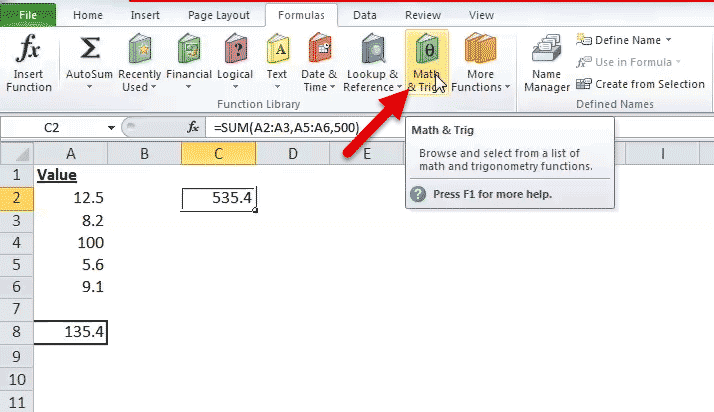
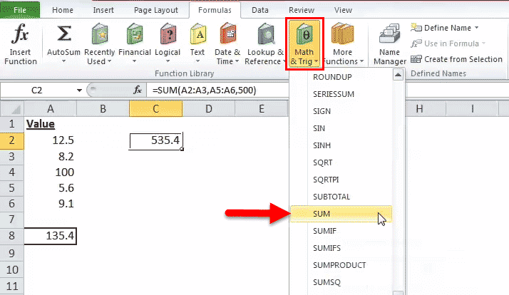
- In the Formulas tab, click the “math & trig” option, as shown in the following image.
2. From the drop-down menu that opens, select the SUM option.
3. In the “function arguments” dialog box, enter the arguments of the SUM function. Click “Ok” to obtain the output.

The AutoSum Option in Excel
The AutoSum option is the fastest way to add numbers in a range of cells. It automatically enters the SUM formula in the selected cell.
Let us work on an example to understand the working of the AutoSum option. We want to sum the list of values in A2:A7, shown in the succeeding image.
The steps to use the AutoSum command are listed as follows:
- Select the blank cell immediately following the cell to be summed up. Choose the cell A8.

- In the Home tab, click “AutoSum”. Alternatively, press the shortcut keys “Alt+=” together and without the inverted commas.

- The SUM formula appears in the selected cell. It shows the reference of the cells that have been summed up.

- Press the “Enter” key. The output appears in cell A8, as shown in the following image.


How to Use the SUM Function in Excel?
Let us consider a few examples to understand the usage of the SUM function. The examples #1 to #5 show an image containing a list of numeric values.
Example #1
We want to sum the cells A2 and A3 shown in the succeeding image.
Apply the formula “=SUM(A2, A3).” It returns 20.7 in cell C2.

Example #2
We want to sum the cells A3, A5, and the number 45 shown in the succeeding image.
Apply the formula “=SUM (A3, A5, 45).” It returns 58.8 in cell C2.

Example #3
We want to sum the cells A2, A3, A4, A5, and A6 shown in the succeeding image.
Apply the formula “=SUM (A2:A6).” It returns 135.4 in cell C2.

Example #4
We want to sum the cells A2, A3, A5, and A6 shown in the succeeding image.
Apply the formula “=SUM (A2:A3, A5:A6).” It returns 35.4 in cell C2.

Example #5
We want to sum the cells A2, A3, A5, A6, and the number 500 shown in the succeeding image.
Apply the formula “=SUM (A2:A3, A5:A6, 500).” It returns 535.4 in cell C2.

The Usage of the SUM Excel Function
The rules governing the usage of the function are listed as follows:
- The arguments supplied can be numbers, arrays, cell references, constants, ranges, and the results of other functions or formulas.
- While providing a range of cells, only the first range (cell1:cell2) is required.
- The output is numeric and represents the sum of values supplied.
- The arguments supplied can go up to a total of 255.
Note: The SUM excel function returns the “#VALUE!” error if the criterion supplied is a text string longer than 255 characters.
The Limitations of the SUM Function in Excel
The drawbacks of the function are listed as follows:
- The cell range supplied must match the dimensions of the source.
- The cell containing the output must always be formatted as a number.
The Nesting of the SUM Excel Function
The built-in formulas of Excel can be expanded by nesting one or more functions inside another function. This permits multiple calculations to take place in a single cell of the worksheet.
The nested function acts as an argument of the main or the outermost function. Excel calculates the innermost function first and then moves outwards.
For example, the following formula shows the SUM function nested within the ROUND functionThe ROUNDUP excel function calculates the rounded value of the number to the upward side or the higher side. In other words, it rounds the number away from zero. Being an inbuilt function of Excel, it accepts two arguments–the “number” and the “num_of _digits.” For example, “=ROUNDUP(0.40,1)” returns 0.4.
read more:

For the given formula, the output is calculated as follows:
- First, the sum of the values in cells A1 to A6 is computed.
- Next, the resulting number is rounded to three decimal places.
With Microsoft Excel 2007, nested functions up to 64 levels are permitted. Prior to this version, one could nest functions only till 7 levels.
Frequently Asked Questions
1. Define the SUM function of Excel.
The SUM function helps add the numerical values. These values can be supplied to the function as numbers, cell references, or ranges. The SUM function is used when there is a need to find the total of specified cells.
The syntax of the SUM excel function is stated as follows:
“SUM(number1,[number2] ,…)”
The “number1” and “number2” are the first and second numeric values to be added. The “number1” argument is mandatory while the remaining values are optional.
In the SUM function, the range to be summed can be provided, which is easier than typing the cell references one by one. The AutoSum option provided in the Home or Formulas tab of Excel is the simplest way to sum two numbers.
Note: The numeric value provided as an argument can be either positive or negative.
2. How to sum the values of filtered data in Excel?
To add the values of filtered data, use the SUBTOTAL function. The syntax of the function is stated as follows:
“SUBTOTAL(function_num,ref1,[ref2],…)”
The “function_num” is a number ranging from 1 to 11 or 101 to 111. It indicates the function to be used for the SUBTOTALThe SUBTOTAL excel function performs different arithmetic operations like average, product, sum, standard deviation, variance etc., on a defined range.read more. The functions used can be AVERAGE, MAX, MIN, COUNT, STDEV, SUM, and so on.
The “ref1” and “ref2” are the cells or ranges to be added.
The “function_num” and “ref1” arguments are mandatory. The “function_num” 109 is used for adding the visible cells of filtered data.
Let us consider an example.
• The sales revenue generated by A and B of team X are:
$1,240 and $3,562 given in cells C2 and C3 respectively
• The sales revenue generated by C and D of team Y are:
$2,351 and $4,109 given in cells C4 and C5 respectively
We filter only team X rows and apply the formula “SUBTOTAL(109,C2:C3).” It returns $4,802.
Note: Alternatively, the AutoSum property can be used to sum the filtered cells.
3. State the benefits of using the SUM function in Excel.
The benefits of using the SUM function are listed as follows:
• It helps obtain the totals of ranges irrespective of whether the cells are contiguous or non-contiguous.
• It ignores the empty cells and text values entered in a cell. In such cases, it returns an output representing the sum of the remaining numbers of the range.
• It automatically updates to include the addition of a row or a column.
• It automatically updates to exclude the deletion of a row or column.
• It eliminates the difficulty associated with typing manual entries.
• It makes the output more readable by allowing the cell to be formatted as a number.
SUM Function in Excel Video
Recommended Articles
This has been a guide to the SUM function in Excel. Here we discuss how to use Sum Formula along with step by step examples and FAQs. You can download the Excel template from the website. Take a look at these useful functions of Excel–
- SUMIFS with Multiple Criteria
- SUMX in Power BISUMX is a function in power BI which returns the sum of expression from a table. It is an inbuilt mathematical function. The syntax used for this function is SUMX(,).read more
- TEXT Function
- Concatenate Excel Function
- Excel Alternate Row ColorThe two different methods to add colour to alternative rows are adding alternative row colour using Excel table styles or highlighting alternative rows using the Excel conditional formatting option.read more
Reader Interactions
The SUM function concern into the category «Mathematical». Press the combination of hot keys SHIFT + F3 to call of the function wizard, and you will quickly search out it there.
The using of this function significantly expands to the possibilities of the process of summing the values of the cells in Excel. We look at the possibilities and settings for the summing several ranges practically.
How in the Excel table to calculate the amount of the column?
Sum up the value of the cells A1, A2 and A3 using the summation function and at the same time we will learn what the sum function is used for.
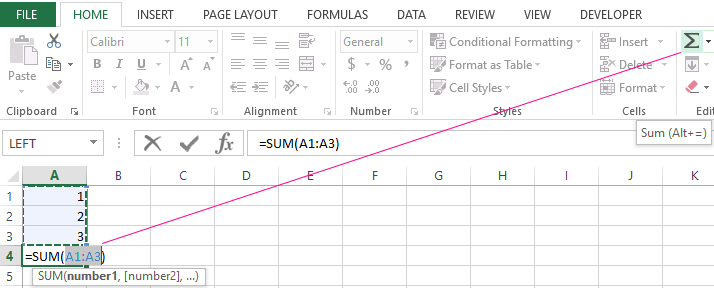
- After entering the numbers, go to the cell A4. On the «Home» tab, select the «Sum» tool in the «Edit» section (or press the ALT + = hot keys combination).
- The range of the cells is recognized automatically. The reference addresses are already entered in the parameters (A1:A3). The user only remains to press Enter.
Consequently, the calculation result is displayed in the cell A4. The function itself and its parameters can be seen in the formula bar.
The notation. Instead of using the «Sum» tool on the main panel, you can directly enter the function with parameters manually in the cell A4. The result will be the same.
The Automatic Range Recognition Correction
When you enter of the function using the button on the toolbar or using the function wizard (SHIFT + F3), the SUM () function refers to the group of formulas «Mathematical». Automatically recognized ranges are not always suitable for the user: its can be quickly and easily repaired if necessary.
Suppose we need to sum several ranges of cells, as shown in the picture:
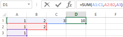
- Go to the cell D1 and select the «Sum» tool.
- While holding the CTRL key, select the range A2:B2 and the cell A3.
- After selecting of the ranges, press Enter and in the cell D4 immediately displays the result of summing the values of cells in all ranges.
Pay attention to the syntax in the function parameters when selecting multiple ranges, that are divided among themselves (;).
In the SUM formula parameters may contain:
- the links to individual cells;
- the references to ranges of the cells both contiguous and non-adjacent;
- the integer and fractional numbers.
In the function parameters, all arguments must be separated by a semicolon.
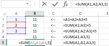
For the illustrative example, let’s consider different variants of summation of values of cells, that give the same result. To do this, fill the cells A1, A2 and A3 with numbers 1, 2 and 3 respectively. And fill the range of the cells B1:B5 with the following formulas and functions:
For any variant, we get the same result of calculation — the number 11. Continue successively with the cursor from B1 and to B5. In each cell, press F2 to see the color highlighting of the links for a more intuitive analysis of the syntax for writing parameters.
The contemporaneous summation of the columns
In Excel, you can simultaneously sum several adjacent and non-adjacent columns.
Fill in the columns, as shown in the picture:
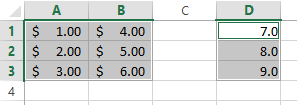
- Select the range A1:B3 and holding down the CTRL key also select the column D1:D3.
- On the «HOME» panel, click the «Sum» tool (or press ALT + =).
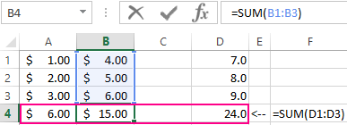
Under each column, the SUM () was automatically added. Now in the cells A4;B4 and D4 the result of the summation of each column is displayed. This is the fastest and most convenient method.
The notation. This function automatically substitutes the format of the cells it sums.
Return value
The sum of values supplied.
Usage notes
The SUM function returns the sum of values supplied. These values can be numbers, cell references, ranges, arrays, and constants, in any combination. SUM can handle up to 255 individual arguments.
The SUM function takes multiple arguments in the form number1, number2, number3, etc. up to 255 total. Arguments can be a hardcoded constant, a cell reference, or a range. All numbers in the arguments provided are summed. The SUM function automatically ignores empty cells and text values, which makes SUM useful for summing cells that may contain text values.
The SUM function will sum hardcoded values and numbers that result from formulas. If you need to sum a range and ignore existing subtotals, see the SUBTOTAL function.
Examples
Typically, the SUM function is used with ranges. For example:
=SUM(A1:A9) // sum 9 cells in A1:A9
=SUM(A1:F1) // sum 6 cells in A1:F1
=SUM(A1:A100) // sum 100 cells in A1:A100
Values in all arguments are summed together, so the following formulas are equivalent:
=SUM(A1:A5)
=SUM(A1,A2,A3,A4,A5)
=SUM(A1:A3,A4:A5)
In the example shown, the formula in D12 is:
=SUM(D6:D10) // returns 9.05
References do not need to be next to one another. For example:
=SUM(A1,F13,E100)
Sum with text values
The SUM function automatically ignores text values without returning an error. This can be useful in situations like this, where the first formula would otherwise throw an error.
Keyboard shortcut
Excel provides a keyboard shortcut to automatically sum a range of cells above. You can see a demonstration in this video.
Notes
- SUM automatically ignores empty cells and cells with text values.
- If arguments contain errors, SUM will return an error.
- The AGGREGATE function can sum while ignoring errors.
- SUM can handle up to 255 total arguments.
- Arguments can be supplied as constants, ranges, named ranges, or cell references.
Presentation of the SUM function
SUM is the most common formula used in Excel and also the simplest to use. We will see in this page, different methods to perform a SUM of your data.
Don’t select many cells
When you work with Excel for the very first time, many people start to create their first formula by selecting many cells
=A1+A2+A3+A4+ …
The calculation will be correct for sure but what a waste of time, especially if you have hundreds of cells to add 😤😱😡 If you have to calculate the sum of many cells in a quick way, it’s much better to use the function SUM.
How to work with SUM in Excel?
Write the formula in the cell
To perform a SUM function in Excel
- You simply start with the = sign in your cell
- Then, you enter the word SUM
- Then you open a parenthesis.
=SUM(
- Select all the cells that you want to include in your sum
=SUM(A1:A5
- Don’t forget to close the parenthesis
=SUM(A1:A5)

Using the icon bar
Instead of writing the formula directly in the cell, you can use the symbol Sigma in the ribbon (tab Home)

The method is simple. You can either
- Select the cell to add and then click on the icon
- Or, select the cells under your range of cells you want to add and then press

Shortcut
You can also insert the function SUM with the shortcut Alt+=
| Alt + = | Insert the function SUM in your active cell |
Dynamic sum
You can create a dynamic sum by using the INDEX function. This is more for advanced Excel users

Author: Oscar Cronquist Article last updated on March 23, 2023
The SUM function in Excel allows you to add values, the function returns the sum in the cell it is entered in. The SUM function is cleverly designed to ignore text and boolean values, adding only numbers.
Excel Function Syntax
SUM(number1, [number2], …)
Arguments
| number1 | Required. A constant, cell reference or an array that contains numerical values you want to add. |
| [number2] | Optional. Up to 254 additional arguments. |
The SUM function lets you add values in cell ranges, arrays, constants. You can have up to 255 different arguments.
Table of Contents
- How to add numbers in a column and return a total (SUM function)?
- How to add numbers in an array (SUM function)?
- How to sum specific cells?
- How to sum numbers from multiple cell ranges (SUM function)?
- How to sum a column with text (SUM function)?
- How to sum boolean values?
- How to create a running total (SUM function)?
- How to sum numbers based on a condition/label/item/category?
- SUM with multiple conditions
- How to sum only visible cells?
- How to sum a filtered column?
- How to sum the entire column?
- How to sum a row?
- How to sum across worksheets?
- How to sum by color?
- How to sum absolute values?
- How to use the SUM function in a macro — VBA example
- What is the shortcut key for the SUM function?
- How to sum values greater than smaller than?
- How to sum values below/above 0 (zero)?
- How to limit SUM function?
- How to sum a column and ignore errors?
- How to sum values by date?
- How to sum values by week?
- How to sum values by month?
- How to sum values by year?
- How to sum values between two dates?
- How to create a reverse running total?
- Get excel *.xlsm file
1. How to add numbers in a column (SUM function)?
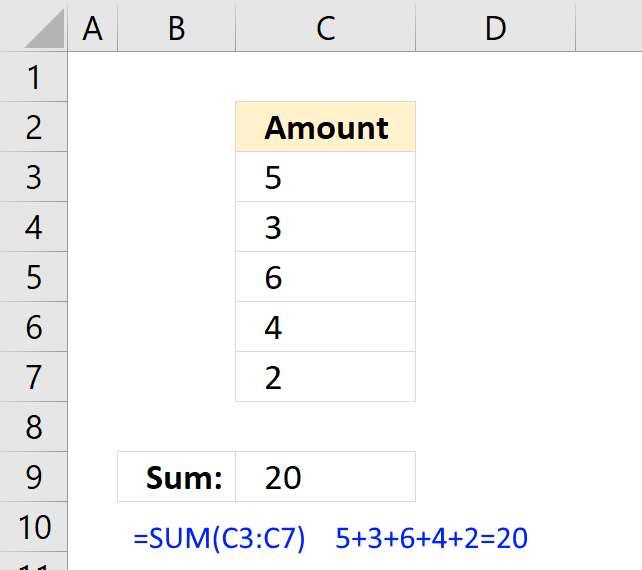
The SUM function lets you add values in a cell range, like this = SUM(B3:B7), instead of adding values in a formula using the plus sign, like this =B3+B4+B5+B6+B7.
The SUM function lets you type one or multiple cell ranges, in this example only cell range B3:B7 is entered as an argument. See the above picture.
Check out the shortcut key to automatically sum a column.
Back to top
2. How to add numbers in an array (SUM function)?
An array is multiple values enclosed with a beginning and ending curly bracket, you can easily convert a cell range to an array. See instructions below.
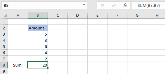
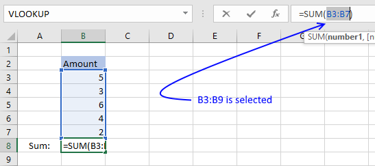
Select a cell and type =SUM(B3:B9)
Press with left mouse button on in the formula bar and select B3:B9.
Press F9 and the cell range is converted to an array, like this: =SUM({5,3,6,4,2})
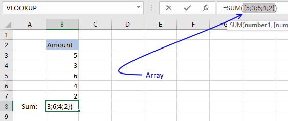
Press Enter.
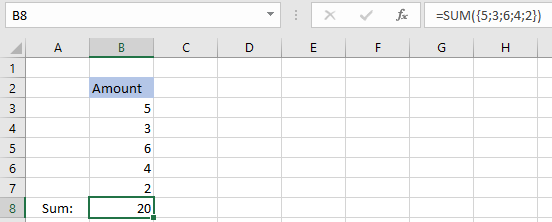
The SUM function adds the values in the array 5+3+6+4+2 = 20. When you convert a cell range to values you hard-code or create constants in your formula, meaning they never change unless you change the values in the formula.
Cell references on the other hand change if you change the values on a worksheet.
I recommend reading this post: Learn the basics of Excel arrays , if you want to learn more about array formulas.
Back to top
3. How to sum specific cells?

The SUM function allows you to add values from the cells you select. The trick is to press and hold the CTRL key while selecting specific cells to sum. Here are the steps in greater detail:
- Doublepress with left mouse button on a cell, the prompt shows up.
- Type =SUM(
- Press and hold CTRL-key.
- Press with left mouse button on with the left mouse button on cells you want to sum.
- Release CTRL-key.
- Add an ending parenthesis )
- Press Enter.

You can also sum cells based on a condition applied to an adjacent column.
Back to top
4. How to sum numbers in multiple cell ranges?
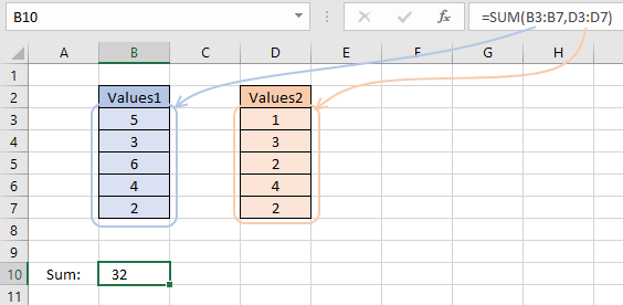
If you want to add values in multiple cell ranges you simply use a comma between arguments. Check your regional settings if a comma doesn’t work for you. You are allowed to have up to 255 arguments in one SUM function.
- Doublepress with left mouse button on a cell, the prompt shows up.
- Type =SUM(
- Press and hold CTRL-key.
- Press and hold with the left mouse button.
- Drag with mouse to select the cell range.
- Release left mouse button.
- Go back to step 4 until all cell ranges have been selected.
- Release CTRL-key.
- Add an ending parenthesis )
- Press Enter.
Back to top
5. How to sum a column with text?
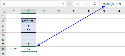
The formula in cell B8 adds the values in cell range B3:B7. 5 + AA + 6 + 4 +2 = 17. The SUM function ignores text strings, in this case AA.
The SUM function ignores text values and boolean values but not error values.
Note, the SUM function ignores numbers stored as text. The image below shows the SUM function in cell B8. Only number 4 is included in the total of cells in cell range B3:B7.

Excel shows numbers stored as text differently, see image above. Text values are aligned left in the cell and numbers are aligned right. Cells containing numbers stored as text show a green arrow in the upper left corner of the cell.
Back to top
6. How to sum boolean values?
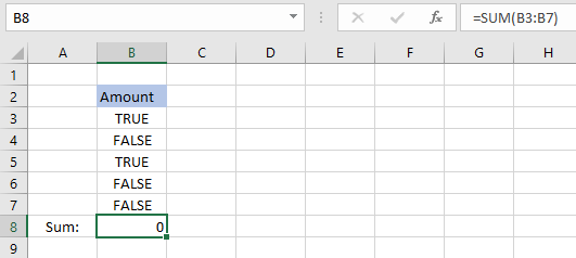
Cell range B3:B7 contains boolean values, TRUE or FALSE, however, the SUM function can’t add boolean values unless they are converted to their numerical equivalents.
There are multiple solutions to this problem, here are a few:
Formula in cell B8:
=SUM(—(B3:B7))
Formula in cell B8:
=SUM(B3:B7+0)
Formula in cell B8:
=SUM(B3:B7*1)
They all convert boolean values to numerical values.
They need to be entered as array formula, because they do calculations to a cell range containing multiple cells.
Instructions on how to enter an array formula.
- Double press with left mouse button on cell B8
- Type =SUM(B3:B7*1)
- Press and hold CTRL + SHIFT simultaneously.
- Press Enter once.
- Release all keys.
The formula in the formula bar changes to {=SUM(B3:B7*1)}
These curly brackets tell you that you have created an array formula, don’t enter these characters yourself.
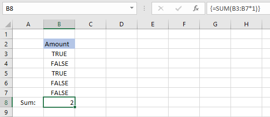
The formula returns 2 because TRUE equals 1 and FALSE equals 0. 1+0+1+0+0 = 2.
Note, you can use the SUMPRODUCT function if you don’t want to use array formulas.
Regular formula in cell B8:
=SUMPRODUCT(B3:B7*1)
Back to top
7. How to create a running total?
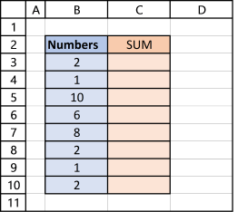
The image above shows you numbers in column B.
Enter this formula in cell C3:
=SUM($B$3:B3)
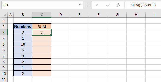
Make sure you get the dollar signs right, they are important. The cell reference changes as you copy the formula and paste it to cells below.
Select cell C4 and see how the formula changed in the formula bar. The part of the cell reference without dollar signs changed from B3 to B4.
That part is a relative cell reference and the part with dollar signs is an absolute cell reference.
Read more here: Absolute and relative cell references
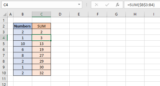
This makes the SUM function use a cell reference that grows, in other words, it includes more and more cells creating a running total.
Formula in cell C4 adds numbers from both cell B3 and B4. The formula grows even further in cell C5 and it keeps growing in cells below.
Note, you can double press with left mouse button on the dot in the lower right corner of the cell to automatically copy the cell and paste it to cells below as far as there are populated cells in the adjacent column.

You can also easily create a reverse running total using two SUM functions, it adds values from the bottom going up to the top.
Back to top
8. How to sum with a condition [array formula]
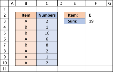
The picture above shows you two columns, column B contains text values and column C contains numbers. The formula demonstrated here allows you to sum by another column.
The formula in cell F3 lets you add numbers in column C if their adjacent value is equal to the value in cell F2:
=SUM((B3:B10=F2)*C3:C10)
This formula is entered as an array formula unless you are using Excel 365. I recommend the SUMIF function built exactly for this without entering the formula as an array formula.
Explaining formula in cell F3
Step 1 — Logical expression
The equal sign in B3:B10=F2 lets you compare the values in cell range B3:B10 with the value in cell F2. The equal sign is a logical operator, often used in IF functions.
{«A»;»B»;»B»;»A»;»B»;»A»;»A»;»A»}=»B»
This logical test returns an array of boolean values:
{FALSE; TRUE; TRUE; FALSE; TRUE; FALSE; FALSE; FALSE}
Step 2 — Multiply array with cell range
The parentheses (B3:B10=F2) make sure this part of the formula is calculated first before multiplying with the numbers in cell range C3:C10.
(B3:B10=F2)*C3:C10
becomes
{FALSE; TRUE; TRUE; FALSE; TRUE; FALSE; FALSE; FALSE}*C3:C10
becomes
{FALSE; TRUE; TRUE; FALSE; TRUE; FALSE; FALSE; FALSE}*{2; 1; 10; 6; 8; 2; 1; 2}
FALSE is equal to 0 (zero) and TRUE is equal to 1.
{FALSE; TRUE; TRUE; FALSE; TRUE; FALSE; FALSE; FALSE}*{2; 1; 10; 6; 8; 2; 1; 2}
becomes
{0; 1; 1; 0; 1; 0; 0; 0}*{2; 1; 10; 6; 8; 2; 1; 2}
becomes
{0*2;1*1;1*10;0*6;1*8;0*2;0*1;0*2}
and returns
{0; 1; 10; 0; 8; 0; 0; 0}
Step 3 — Sum numbers
The SUM function then adds the number in the array:
SUM({0; 1; 10; 0; 8; 0; 0; 0})
and returns 19 in cell F3. 1+10+8 = 19
Back to top
9. Sum with multiple conditions [array formula]
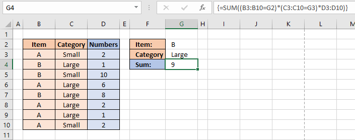
Adding a second condition to the formula is easy. Simply add your condition to the formula enclosed with parentheses.
=SUM((B3:B10=G2)*(C3:C10=G3)*D3:D10)
This formula is entered as an array formula unless you are using Excel 365. I recommend the SUMIFS function built exactly for this without the need for an array formula.
Explaining formula in cell G4
Step 1 — First condition
The equal sign allows you to compare cells to each other.
B3:B10=G2
becomes
{«A»;»B»;»B»;»A»;»B»;»A»;»A»;»A»}=»B»
and returns
{FALSE; TRUE; TRUE; FALSE; TRUE; FALSE; FALSE; FALSE}
Step 2 — Second condition
C3:C10=G3
becomes
{«Small»;»Large»;»Small»;»Large»;»Large»;»Large»;»Large»;»Small»}=»Large»
and returns
{FALSE; TRUE; FALSE; TRUE; TRUE; TRUE; TRUE; FALSE}
Step 3 — Multiply arrays
(B3:B10=G2)*(C3:C10=G3)*D3:D10
becomes
{FALSE; TRUE; TRUE; FALSE; TRUE; FALSE; FALSE; FALSE}*{FALSE; TRUE; FALSE; TRUE; TRUE; TRUE; TRUE; FALSE}*{2;1;10;6;8;2;1;2}
becomes
{0; 1; 0; 0; 1; 0; 0; 0}*{2; 1; 10; 6; 8; 2; 1; 2}
and returns
{0;1;0;0;8;0;0;0}
Step 4 — Sum values in the array
SUM((B3:B10=G2)*(C3:C10=G3)*D3:D10)
becomes
SUM({0;1;0;0;8;0;0;0})
and returns 9.
The SUMPRODUCT function allows you to perform the same calculation without the need for entering the formula as an array formula.
=SUMPRODUCT((B3:B10=G2)*(C3:C10=G3)*D3:D10)
Back to top
10. How to sum only visible cells?
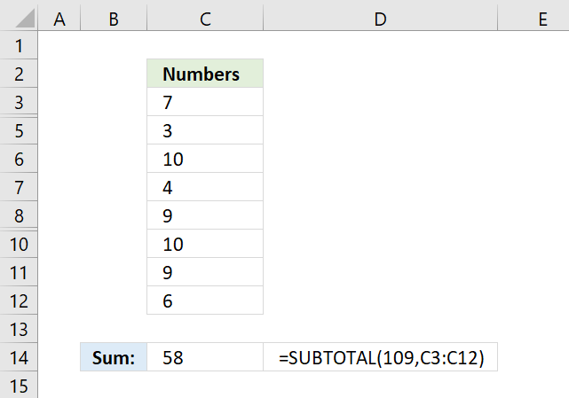
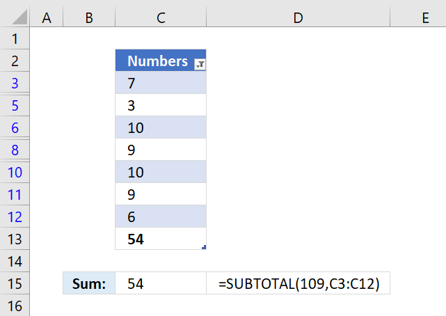
The SUBTOTAL function lets you sum values in a cell range that have some rows hidden or filtered, the picture above shows a cell range that has row 4 and 9 hidden. The usual SUM function won’t work in this case, you need the SUBTOTAL function:
=SUBTOTAL(109,C3:C12)
The first argument allows you to pick a function number that determines how the SUBTOTAL function behaves. In this case, 109 sums all visible cells in a cell range.
To hide a value simply press with right mouse button on on a row number and then press with left mouse button on «Hide» to hide the entire row. Select the rows around a hidden row and then press with right mouse button on on them to open a menu, there press with left mouse button on «Unhide» to show the value again.
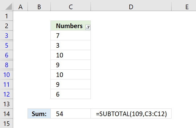
The picture above shows filtered values in column C. Excel tells you that the cell range is filtered by the color of the row numbers and the icon next to «Numbers» in cell C2.
To apply a filter to a column simply select the cell range, go to tab «Data» on the ribbon, press with left mouse button on «Filter» button. A black down-pointing arrow appears next to header name «Numbers», press with left mouse button on it to apply a filter.
The Excel defined table above has a built-in feature that allows you to sum filtered values automatically, all you need to do is select a cell in the table, go to tab «Design» on the ribbon, then press with left mouse button on check-box «Total Row» to show the totals.
Cell C13 in the picture above displays the total for filtered cells. The SUBTOTAL function works just as well if you prefer using an Excel function with an Excel defined table, demonstrated in cell C15.
How to hide / unhide values?

Note, follow these instructions on how to hide and unhide specific rows:
- Press with right mouse button on on row number.
- A popup-menu appears, see image above.
- Press with mouse on Hide or Unhide.
Tip! Press and hold CTRL key while selecting rows to hide/unhide multiple values at the same time.
Back to top
11. How to sum a filtered column?

The image above shows numbers in cell range C3:C7, however, a filter is applied and rows 4 and 6 are hidden. The SUM function in cell C9 can’t ignore filtered values, you need the SUBTOTAL function to sum filtered numbers.
Formula in cell C10:
=SUBTOTAL(109, B3:B7)
Back to top
12. How to sum the entire column?

The image above shows a formula that adds all values in a column and returns a total.
Formula in cell E2:
=SUM(B:B)
The cell reference is B:B meaning that all numerical values in column B are included in the total.
Back to top
13. How to sum a row?

The image above shows a formula that adds all values in a row and returns a total.
Formula in cell C4:
=SUM(2:2)
The cell reference is 2:2 meaning that all numerical values in row 2 are included in the total.
Back to top
14. How to sum across worksheets?

The image above shows a formula that adds values located in cell C3 across three different worksheets. For this to work values you want to add must be located in the same cell across all worksheets.
Formula in cell C3:
=SUM(‘across sheets1:across sheets3’!C3)
Here are the steps I did to create the formula above:
- Doublepress with left mouse button on cell C3, the prompt is shown.
- Type =SUM(
- Go to the first worksheet.
- Press with mouse on the cell containing the value you want to add.
- Press and hold SHIFT key.
- Select the last worksheet you want to include in the total.
- Release the SHIFT key.
- Type an ending parenthesis )
- Press Enter.
The image below shows the tabs I selected to create the formula above.

Back to top
15. How to sum by color?

The short answer is that there is really no way to sum by background color if you want to use formulas, however, a VBA macro can do it.
The long answer is that there is the GET.CELL function that has some serious flaws, one is that it is outdated and may be removed from Excel by Microsoft whenever they feel like it. I’d rather recommend coloring cells using Conditional Formatting and then using the same condition to sum the cells.
This is what the image above shows, I chose to highlight rows blue if the corresponding cell in column B is equal to item «B». Here is how I did it:
- Select the cells you want to highlight, in the example above cell range B3:C10.
- Go to tab «Home» on the ribbon.
- Press with left mouse button on the Conditional Formatting button.
- Press with left mouse button on «New Rule…». A dialog box appears.

- Press with mouse on «Use a formula to determine which cells to format»
- Press with mouse on field below «Format values where this formula is true:».
- Type =$B3=$F$2
- Press with left mouse button on «Format…» button. A new dialog box appears.

- Press with left mouse button on tab «Fill» on top menu.
- Pick a color.
- Press with left mouse button on OK. The dialog box is closed.
- Press with left mouse button on OK again.


The formula in cell F3 is explained here: How to sum numbers based on a condition/label/item/category?
Back to top
16. How to sum absolute numbers?

The image above shows a formula in cell C8 that converts negative values to positive values and then adds the values.
Formula in cell C8:
=SUM(ABS(C3:C7))
Explaining formula in cell C8
Step 1 — Remove sign
The ABS function converts negative numbers to positive numbers, in other words, the ABS function removes the sign.
ABS(number)
ABS(C3:C7)
becomes
ABS({5; -3; 6; -4; 2})
and returns
{5; 3; 6; 4; 2}
Step 2 — Add values
SUM(ABS(C3:C7))
becomes
SUM({5; 3; 6; 4; 2})
and returns 20. 5+3+6+4+2 = 20
17. How to use the SUM function in a macro (VBA)?
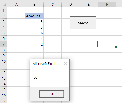
The image above demonstrates a macro that shows a message box with a number representing the total of cell range B3:B7.
'Macro name
Sub HLP()

'Show sum of B3:B7 in a messagebox
MsgBox Application.WorksheetFunction.Sum(Range("B3:B7"))

'Exit macro
End Sub
Microsoft docs: | Application.WorksheetFunction | Sum | Range | Msgbox
Back to top
18. What is the shortcut key for the SUM function?

The animated image above shows how to add totals for a cell range, both vertically and horizontally, using a shortcut key.
The SUM formulas in cell range G3:G7 adds values from the cell to the left of the formula and on the same row.

The SUM formulas in cell range C7:F7 return a total based on the numbers above the formulas in the same column.

Here is how to create the SUM function using a shortcut key:
- Select the cell range containing numbers.
- Press and hold Alt key.
- Press the equal sign =
- Release the Alt key.
If the steps above don’t work for you try Alt + Shift + 0 (zero) keys. It really depends on your keyboard layout which keys you need to press.

The ímage above shows that you can use the shortcut key below numbers in a column.
Back to top
19. How to sum values below/above a threshold?

The image above demonstrates two array formulas in cell E3 and E5 that return a total with values larger or smaller than a given threshold.
Array formula in cell E3:
=SUM(IF(B3:B7>E2, B3:B7, ))
Array formula in cell E6:
=SUM(IF(B3:B7<E2,B3:B7,))
How to enter an array formula
I recommend the SUMIF function built exactly for this without entering the formula as an array formula.
Explaining formula in cell E3
Step 1 — Filter values above a threshold
The IF function returns one value if the logical test is TRUE and another value if the logical test is FALSE.
IF(logical_test, [value_if_true], [value_if_false])
IF(B3:B7>E2, B3:B7, )
becomes
IF({3;9;2;4;6}>5,{3;9;2;4;6},)
becomes
IF({FALSE; TRUE; FALSE; FALSE; TRUE},{3; 9; 2; 4; 6},)
and returns
{0;9;0;0;6}
Step 2 — Sum values
SUM(IF(B3:B7>E2, B3:B7, ))
becomes
SUM({0;9;0;0;6})
and returns 15 in cell E3.
Back to top
20. How to sum values below/above 0 (zero)?

The image above demonstrates two formulas in cells E2 and E3 that return a total with values above and below zero respectively.
Array formula in cell E2:
=SUM(IF(B3:B7>0, B3:B7, ))
Array formula in cell E3:
=SUM(IF(B3:B7<0, B3:B7, ))
How to enter an array formula
I recommend the SUMIF function built exactly for this without entering the formula as an array formula.
Explaining formula in cell E2
Step 1 — Filter values above a 0 (zero)
The IF function returns one value if the logical test is TRUE and another value if the logical test is FALSE.
IF(logical_test, [value_if_true], [value_if_false])
IF(B3:B7>0, B3:B7, )
becomes
IF({1;-2;3;4;-3}>0,{1;-2;3;4;-3},)
becomes
IF({TRUE;FALSE;TRUE;TRUE;FALSE},{1;-2;3;4;-3},)
and returns
{1;0;3;4;0}
Step 2 — Sum numbers
SUM(IF(B3:B7>0, B3:B7, ))
becomes
SUM({1;0;3;4;0})
and returns 8 in cell E2. 1 + 3 + 4 = 8.
Back to top
21. How to limit the SUM function?

The image above demonstrates a formula in cell E3 that sums values in cell range B3:B7 and returns a total that is limited to the number specified in cell E2. In other words, the total can’t be larger than the value in cell E2 but it can be smaller.
The image above also shows a formula in cell E6 that adds values in cell range B3:B7 and returns a total that is limited to the number specified in cell E5. The total can’t be smaller than the value in cell E5 but it can be larger.
Formula in cell E3:
=MIN(E2, SUM(B3:B7))
Formula in cell E6:
=MAX(E5, SUM(B3:B7))
Explaining formula in cell E3
Step 1 — Sum numbers
SUM(B3:B7)
becomes
SUM({5;6;6;7;2})
and returns 26. 5+6+6+7+2=26
Step 2 — Return the smallest number
The MIN function returns the smallest number in a cell range or array.
MIN(E2, SUM(B3:B7))
becomes
MIN(20, 26)
and returns 20. 20 is smaller than 26.
Back to top
22. How to sum a column and ignore errors?

The image above shows a formula in cell C9 that sums numbers in cell range C3:C7 and ignores errors.
Array Formula in cell C9:
=SUM(IFERROR(C3:C7, 0))
Explaining formula in cell C9
Step 1 — Replace errors with 0 (zero)
The IFERROR function lets you handle most formula errors with ease.
IFERROR(value, value_if_error)
IFERROR(C3:C7, 0)
becomes
IFERROR({5;#DIV/0!;6;#NAME?;2})
and returns
{5;0;6;0;2}
Step 2 — Sum values in array
SUM(IFERROR(C3:C7, 0))
becomes
SUM({5;0;6;0;2})
and returns 13 in cell C9. 5+6+2=13
Note that the IFERROR catches all errors and may cause problems if you want to troubleshoot formulas. Why? You can’t find errors.
Back to top
23. Sum values based on a date

The image above shows a formula in cell C11 that sums numbers in cell range C3:C7 if dates in B3:B7 are equal to C10.
Array formula in cell C11:
=SUM(IF(B3:B7=C10, C3:C7, «»))
I recommend the SUMIF function built exactly for this without entering the formula as an array formula.
Explaining formula in cell C9
Step 1 — Logical expression
B3:B7=C10
becomes
{43831;43832;43833;43832;43835}=43832
and returns
{FALSE; TRUE; FALSE; TRUE; FALSE}
Step 2 — Evaluate IF function
The IF function returns one value if the logical test is TRUE and another value if the logical test is FALSE.
IF(B3:B7=C10, C3:C7, «»)
becomes
IF({FALSE; TRUE; FALSE; TRUE; FALSE}, C3:C7, «»)
becomes
IF({FALSE; TRUE; FALSE; TRUE; FALSE}, {1; 3; 5; 2; 4}, «»)
and returns {«»; 3; «»; 2; «»}.
Step 3 — Sum values in the array
SUM(IF(B3:B7=C10, C3:C7, «»))
becomes
SUM({«»; 3; «»; 2; «»})
and returns 5. 3+2 = 5.
Back to top
24. Sum values based on week number

The image above shows a formula in cell C11 that sums numbers in cell range C3:C7 if the corresponding weeks based on the dates in B3:B7 are equal to C10.
Array formula in cell C11:
=SUM(IF(ISOWEEKNUM(B3:B7)=C10, C3:C7, «»))
I recommend the SUMIF function built exactly for this without entering the formula as an array formula.
Explaining formula in cell C9
Step 1 — Calculate week numbers
The ISOWEEKNUM function calculates the number of the ISO week number of the year for a specific date.
ISOWEEKNUM(B3:B7)
becomes
ISOWEEKNUM({43839; 43838; 43835; 43833; 43837})
and returns {2; 2; 1; 1; 2}
Step 2 — Logical expression
ISOWEEKNUM(B3:B7)=C10
becomes
{2; 2; 1; 1; 2}=1
and returns {FALSE; FALSE; TRUE; TRUE; FALSE}.
Step 3 — Evaluate IF function
The IF function returns one value if the logical test is TRUE and another value if the logical test is FALSE.
IF(ISOWEEKNUM(B3:B7)=C10, C3:C7, «»)
becomes
IF({FALSE; FALSE; TRUE; TRUE; FALSE}, C3:C7, «»)
becomes
IF({FALSE; FALSE; TRUE; TRUE; FALSE}, {1; 3; 5; 2; 4}, «»)
and returns {«»; «»; 5; 2; «»}
Step 4 — Sum values in the array
SUM(IF(ISOWEEKNUM(B3:B7)=C10, C3:C7, «»))
becomes
SUM({«»; «»; 5; 2; «»})
and returns 7. 5+2 = 7.
Back to top
25. Sum values by month

The image above shows a formula in cell C11 that sums numbers in cell range C3:C7 if the corresponding weeks based on the dates in B3:B7 are equal to C10.
Array formula in cell C11:
=SUM(IF(MONTH(B3:B7)=C10, C3:C7, «»))
I recommend the SUMIF function built exactly for this without entering the formula as an array formula.
Explaining formula in cell C9
Step 1 — Calculate number representing the position of the month in a year
The MONTH function extracts the month as a number from an Excel date.
1 — January, 2 — February, 3 — March, 4 — April, 5 — May, 6 — June, 7 — July, 8 — August, 9 — September, 10 — October, 11 — November, 12 — December
MONTH(B3:B7)
becomes
MONTH({43839; 43869; 43895; 43864; 43837})
returns
{1; 2; 3; 2; 1}
Step 2 — Logical expression
MONTH(B3:B7)=C10
becomes
{1; 2; 3; 2; 1}=1
and returns {TRUE; FALSE; FALSE; FALSE; TRUE}
Step 3 — Evaluate IF function
The IF function returns one value if the logical test is TRUE and another value if the logical test is FALSE.
IF(MONTH(B3:B7)=C10, C3:C7, «»)
becomes
IF({TRUE; FALSE; FALSE; FALSE; TRUE}, {1; 3; 5; 2; 4}, «»)
and returns {1; «»; «»; «»; 4}
Step 4 — Sum values in the array
SUM(IF(MONTH(B3:B7)=C10, C3:C7, «»))
becomes
SUM({1; «»; «»; «»; 4})
and returns 5. 1 + 4 = 5.
Back to top
26. Sum values by year

The image above shows a formula in cell C11 that sums numbers in cell range C3:C7 if the corresponding weeks based on the dates in B3:B7 are equal to C10.
Array formula in cell C11:
=SUM(IF(YEAR(B3:B7)=C10, C3:C7, «»))
I recommend the SUMIF function built exactly for this without entering the formula as an array formula.
Explaining formula in cell C9
Step 1 — Calculate year based on an Excel date
The YEAR function returns the year from an Excel date.
YEAR(B3:B7)
becomes
YEAR({44205; 43869; 44260; 43864; 44568})
and returns {2021; 2020; 2021; 2020; 2022}
Step 2 — Logical expression
YEAR(B3:B7)=C10
becomes
{2021; 2020; 2021; 2020; 2022}=2020
and returns {FALSE; TRUE; FALSE; TRUE; FALSE}
Step 3 — Evaluate IF function
The IF function returns one value if the logical test is TRUE and another value if the logical test is FALSE.
IF(YEAR(B3:B7)=C10, C3:C7, «»)
becomes
IF({FALSE; TRUE; FALSE; TRUE; FALSE}, {1; 3; 5; 2; 4}, «»)
and returns {«»; 3; «»; 2; «»}
Step 4 — Sum values in array
SUM(IF(YEAR(B3:B7)=C10, C3:C7, «»))
becomes
SUM({«»; 3; «»; 2; «»})
and returns 5. 3 + 2 = 5.
Back to top
27. Sum values between two dates

The image above shows a formula in cell C12 that sums numbers in cell range C3:C7 if dates in B3:B7 are less than or equal to C11 and greater than or equal to C10.
Array formula in cell C12:
=SUM(IF((C10<=B3:B7)*(C11>=B3:B7), C3:C7, «»))
I recommend the SUMIFS function built exactly for this without entering the formula as an array formula.
Explaining formula in cell C9
Step 1 — First logical expression
C10<=B3:B7
becomes
43832<={43831; 43832; 43833; 43834; 43835}
and returns
{FALSE; TRUE; TRUE; TRUE; TRUE}
Step 2 — Second logical expression
C11>=B3:B7
becomes
43834>={43831;43832;43833;43834;43835}
and returns
{TRUE; TRUE; TRUE; TRUE; FALSE}
Step 3 — Multiply arrays
(C10<=B3:B7)*(C11>=B3:B7)
becomes
{FALSE; TRUE; TRUE; TRUE; TRUE}*{TRUE; TRUE; TRUE; TRUE; FALSE}
and returns {0; 1; 1; 1; 0}
Step 4 — Evaluate IF function
The IF function returns one value if the logical test is TRUE and another value if the logical test is FALSE.
IF((C10<=B3:B7)*(C11>=B3:B7), C3:C7, «»)
becomes
IF({0; 1; 1; 1; 0}, C3:C7, «»)
becomes
IF({0; 1; 1; 1; 0}, {1; 3; 5; 2; 4}, «»)
and returns {«»; 3; 5; 2; «»}
Step 5 — Sum values in the array
SUM(IF((C10<=B3:B7)*(C11>=B3:B7), C3:C7, «»))
becomes
SUM({«»; 3; 5; 2; «»})
and returns 10. 3+5+2 = 10.
Back to top
28. How to create a reverse running total?

The image above shows a formula in cell C3 that calculates a running total from the bottom to the top and not the other way around.
Formula in cell C3:
=SUM($B$3:$B$7)-SUM($B$2:B2)
Explaining the formula in cell C3
Step 1 — Calculate the total for the entire cell range
The SUM function allows you to add numerical values, the function returns the sum in the cell it is entered in. The SUM function is cleverly designed to ignore text and boolean values, adding only numbers.
Function syntax: SUM(number1, [number2], …)
SUM($B$3:$B$7)
becomes
SUM({5;4;8;6;1})
and returns
24.
Step 2 — Calculate a running total using absolute and relative cell references
SUM($B$2:B2)
The dollar sign lets you change a relative cell reference to an absolute cell reference, this makes the cell reference grow automatically as the cell is copied to the cells below.
Cell C3: SUM($B$2:B2)
Cell C4: SUM($B$2:B3)
Cell C5: SUM($B$2:B4)
Cell C6: SUM($B$2:B5)
Cell C7: SUM($B$2:B6)
Step 3 — Subtract the total with the running total
The minus sign lets you subtract numbers in an Excel formula.
SUM($B$3:$B$7)-SUM($B$2:B2)
becomes
Cell C3: 24-0 equals 24
Cell C4: 24-5 equals 19
Cell C5: 24-9 equals 15
Cell C6: 24-17 equals 7
Cell C7: 24-23 equals 1
The file is a *.xlsm file (macro-enabled Excel file), it contains a small macro that demonstrates how to use the SUM function in a VBA macro.
The following 59 articles contain the SUM function.
The SUM function function is one of many functions in the ‘Math and trigonometry’ category.