How do you divide cells in excel - Word и Excel - помощь в работе с программами

Excel for Microsoft 365 Excel 2021 Excel 2019 Excel 2016 Excel 2013 More…Less

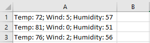
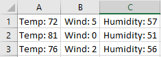
You might want to split a cell into two smaller cells within a single column. Unfortunately, you can’t do this in Excel. Instead, create a new column next to the column that has the cell you want to split and then split the cell. You can also split the contents of a cell into multiple adjacent cells.

See the following screenshots for an example:

Split the content from one cell into two or more cells

Select the cell or cells whose contents you want to split.

Important: When you split the contents, they will overwrite the contents in the next cell to the right, so make sure to have empty space there.
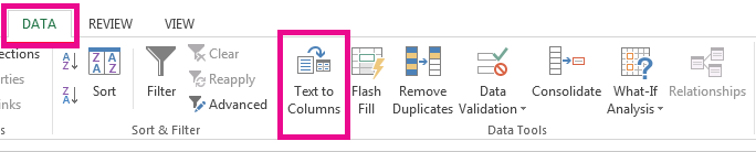
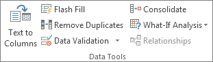
On the Data tab, in the Data Tools group, click Text to Columns. The Convert Text to Columns Wizard opens.
Choose Delimited if it is not already selected, and then click Next.
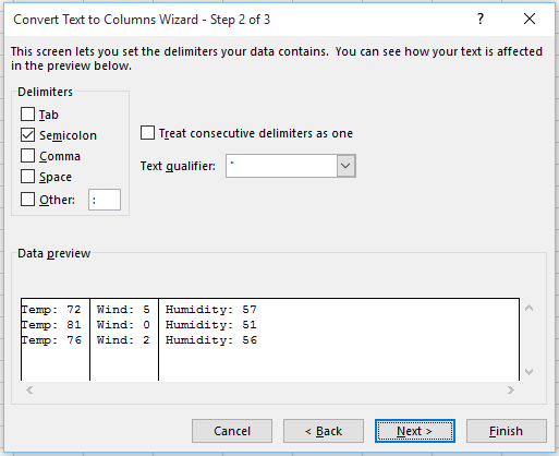
Select the delimiter or delimiters to define the places where you want to split the cell content. The Data preview section shows you what your content would look like. Click Next.
In the Column data format area, select the data format for the new columns. By default, the columns have the same data format as the original cell. Click Finish.

Introduction to Divide Cell in Excel

When we work with the text files in excel, it has all the data in the single row itself instead of having it in different columns. The data, most of the times, is aligned in a single row with some delimiter or separator in it (such as comma, space, etc.). If you open such files in Excel, you’ll not get the data populated across columns for different attributes, which is a problem in its own ways. It makes dividing the cells into different columns extremely important, and that is exactly what we will walk you through in this article.

Data Structure in a Text File:

The data is comma-separated if you see the below screenshot and has the first row as column headers. Below that, there is one blank row and then the data values that are comma-separated as well. This type of data is called as delimited data or data with delimiters (in this case, comma as a delimiter).

Let us see the other data set which we are going to use.

This data set simply consists of EmpID and EmpName, as it seems, and there is no special delimiter in this data as well. For both of these types of data, we need to divide the cells into different columns.

Excel has a Text to Column tool, which helps us divide the cells into different columns.

Examples of Divide Cell in Excel

We will see how it works with two examples in this article.

Example #1 – Divide cells with Delimiter in Excel

See the data below. The same text file is opened with Excel, which we have seen through the above screenshots and has comma-separated values in it within a single row of the sheet.

To divide it into different columns per field value, we need to use the Text to Column utility in Excel.

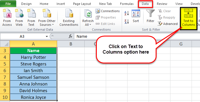
Step 1: Select all the cells from column A (spread across the cells A1 to A12) containing data which is comma-separated.

Step 2: Navigate to the Data tab under the Excel ribbon, which is placed at the uppermost corner of the worksheet and click on it.

Step 3: As soon as you click on the Data tab, you’ll see different options associated with the data using which we can manipulate the data in Excel. However, you need to navigate to the Data Tools group, under which you’ll see Text to Column as an option.

As soon as you click on the Text to Column option, you’ll see Convert Text to Column Wizard popping up on your excel screen, as shown below:

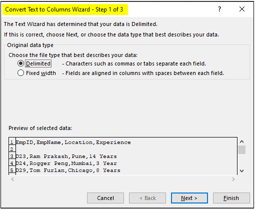
By default, the Delimited option is checked for you. Since our data has a delimiter (comma), we will go with the same selection. Click on the Next > button.

Step 4: Under the Delimiters section, tick the select Comma option (since we have comma-separated data with us). You have different delimiter options such as Tab, Semicolon, Space, etc.; if your data has any delimiter apart from these standard ones, you can use other options to add it as a delimiter for the data to be divided. Since we have a comma with us, we will use the comma as a delimiter. Once you click on the comma, you can see the cell values are divided into separate columns after each comma under the Data preview section. Click on the Next button after done.

Once you click on the next option, you’ve several options that will allow you to either change the column data type for various columns the data gets split in. Ex. Whether you wanted to store any specific column as a Text or Date format or choose not to import that column with the option, do not import the column (skip) option. Well, these are the options; right now, we are not going to use to and just will use the standard Text to Column settings, in which the Column Data Format is set as General.

Step 5: Set the Column data format as General by clicking the General radio button. Under the Destination: section set the destination as cell A1 and click on the Finish option to complete the dividing data into cells procedure.

Once you click on the Finish option, you can see data divided across different columns, as shown in the screenshot below:

You can see the data which was in a single cell with a comma as a separator or delimiter is now populated across the different columns such as EmpID (column A), EmpName (column B), Location (column C) and Experience (column D).

This is one way to divide cells in Excel when you have delimited data.

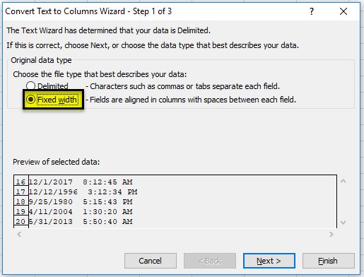
Example #2 – Divide cells with Fixed Width in Excel

The Other example is something where you don’t have any delimiter but a data with fixed with and you need to divide the cells containing that data into different columns.

See the data below:

Step 1: Follow the first three steps from the previous example (Example 1) as it is to be able to open the Text to Column Wizard in Excel, which helps in dividing the cells.

Step 2: Now, as soon as the Convert Text to Columns Wizard gets opened, you need to click the Fixed Width radio button instead of the Delimited (which is set by default). Click on the Next button.

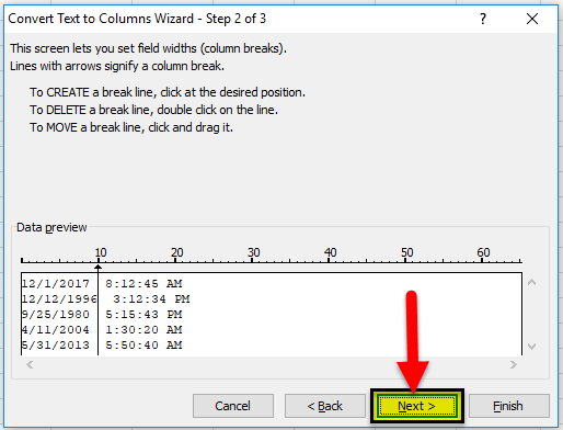
Step 3: After you click on the Next button, you can make the split after a specific length. For Example, we can make a split after the first three characters, which are part of EmpID. See the screenshot below. After you are happy with the split made, click on the Next button.

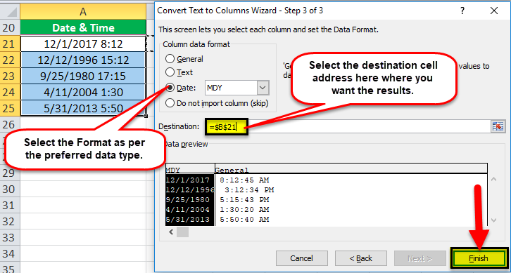
Step 4: On the next screen, you can set the data type as General, Date, etc. And set the Destination Range as well. Once done, you can click on the Finish button. See the screenshot below:

Once you click on the Finish button, you can see the data divided into two different columns, as shown below:

This is how we can divide cells in Excel into different columns using Text to Column wizard.

Things to Remember

For dividing the cells, your data should have a common delimiter for all the fields. Otherwise, it is not possible to divide the data into different columns.
If the data doesn’t have a delimiter, you can use the Fixed Width option as well. However, your data should have a fixed number of characters where a split can happen for that to happen. For Ex. after every third character, you may create a split (as shown in Example 2.)

How do you divide cells?

Mitosis is a fundamental process for life. During mitosis, a cell duplicates all of its contents, including its chromosomes, and splits to form two identical daughter cells.

How do I divide a whole number in Excel?

Tip: If you want to divide numeric values, you should use the “/” operator as there isn’t a DIVIDE function in Excel. For example, to divide 5 by 2, you would type =5/2 into a cell, which returns 2.5. The QUOTIENT function for these same numbers =QUOTIENT(5,2) returns 2, since QUOTIENT doesn’t return a remainder.

What is the formula of division?

A divisor is represented in a division equation as: Dividend ÷ Divisor = Quotient. Similarly, if we divide 20 by 5, we get 4.

How do I multiply two columns in Excel?

For example, to multiply values in columns B, C and D, use one of the following formulas: Multiplication operator: =A2*B2*C2. PRODUCT function: =PRODUCT(A2:C2) Array formula (Ctrl + Shift + Enter): =A2:A5*B2:B5*C2:C5.

Is there a divide function in Excel?

Note: There is no DIVIDE function in Excel.

How do I split a group of numbers in Excel?

Highlight the range that you want to divide all numbers by 15 and right-click, choose Paste Special from the menu. 3. In the Paste Special dialog box, click All option in the Paste section, select the Divide option in the Operation section, and finally click the OK button.

How do you show a number divided by 1000 in Excel?

To do this, follow these steps:

Select the range of cells you want to format.
Right-click the range to display a Context menu, from which you should choose Format Cells.
Make sure the Number tab is displayed.
In the Category list, choose Custom.
In the Type box enter “##,##0.00,” (without the quote marks).
Click OK.

How do I split a column into two parts in Excel?

In This Article

Select the data that needs dividing into two columns.
On the Data tab, click the Turn to Columns button.
Choose the Delimited option (if it isn’t already chosen) and click Next.
Under Delimiters, choose the option that defines how you will divide the data into two columns.
Click Next.
Click Finish.

How do you divide by 1000?

To divide by 1000, move all digits in a number 3 place value columns to the right.

To divide a number by 1000, move all of its digits 3 place value columns to the right.
In this example we have 604 ÷ 1000.
The ‘6’ in the hundreds column moves to the tenths column, immediately after the decimal point.

How do you multiply in Excel formula?

To write a formula that multiplies two numbers, use the asterisk (*). To multiply 2 times 8, for example, type “=2*8”. Use the same format to multiply the numbers in two cells: “=A1*A2” multiplies the values in cells A1 and A2.

How do you equally space cells in sheets?

How to distribute columns evenly in Google Sheets

Select the columns that you want to evenly space.
Right-click on the top of one of the selected columns, then click “Resize column…”
Enter the new column width in pixels (Defaults is 100), then click “OK”

How do I split a cell into multiple rows?

Split cells

Click in a cell, or select multiple cells that you want to split.
Under Table Tools, on the Layout tab, in the Merge group, click Split Cells.
Enter the number of columns or rows that you want to split the selected cells into.

How do you add and divide cells in Excel?

Enter the Formula Using Pointing

Type an equal sign ( = ) in cell B2 to begin the formula.
Select cell A2 to add that cell reference to the formula after the equal sign.
Type the division sign ( / ) in cell B2 after the cell reference.
Select cell A3 to add that cell reference to the formula after the division sign.

How do I split a whole column in sheets?

Using the DIVIDE Formula
Click on an empty cell and type =DIVIDE(,) into the cell or the formula entry field, replacing and with the two numbers you want to divide. Note: The dividend is the number to be divided, and the divisor is the number to divide by.

What is the shortcut to divide in Excel?

You can insert a division symbol by shortcut key in Excel. Select a cell you will insert division symbol, hold the Alt key, type 0247 and then release the Alt key. Then you can see the ÷ symbol is showing in the selected cell. Note: The number 0247 you typed must in the numeric keypad.

Источник

Содержание

Distribute the contents of a cell into adjacent columns
Need more help?
Split Cells in Excel
How to Split a Cell in Excel?
Example #1–Split by “Delimited” Option
Example #2–Split by “Fixed Width” Option
Frequently Asked Questions
Recommended Articles
How to divide numbers and cells in Microsoft Excel to make calculations and analyze data
Check out the products mentioned in this article:
MacBook Pro (From $1,299.99 at Best Buy)
Lenovo IdeaPad 130 (From $299.99 at Best Buy)
How to divide two numbers in Excel
How to divide a column of values by a constant

Distribute the contents of a cell into adjacent columns

You can divide the contents of a cell and distribute the constituent parts into multiple adjacent cells. For example, if your worksheet contains a column Full Name, you can split that column into two columns—a First Name column and Last Name column.

For an alternative method of distributing text across columns, see the article, Split text among columns by using functions.

You can combine cells with the CONCAT function or the CONCATENATE function.

Follow these steps:

Note: A range containing a column that you want to split can include any number of rows, but it can include no more than one column. It’s important to keep enough blank columns to the right of the selected column, which will prevent data in any adjacent columns from being overwritten by the data that is to be distributed. If necessary, insert a number of empty columns that will be sufficient to contain each of the constituent parts of the distributed data.

Select the cell, range, or entire column that contains the text values that you want to split.

On the Data tab, in the Data Tools group, click Text to Columns.

Follow the instructions in the Convert Text to Columns Wizard to specify how you want to divide the text into separate columns.

Note: For help with completing all the steps of the wizard, see the topic, Split text into different columns with the Convert Text to Columns Wizard, or click Help in the Convert to Text Columns Wizard.

This feature isn’t available in Excel for the web.

If you have the Excel desktop application, you can use the Open in Excel button to open the workbook and distribute the contents of a cell into adjacent columns.

Need more help?

You can always ask an expert in the Excel Tech Community or get support in the Answers community.

Источник

Split Cells in Excel

Splitting Cells in Excel refers to dividing its content into two or more separate cells. Splitting cells is often required when large datasets are imported in excel from external sources. In such cases, there is a need to create separate columns for similar data values.

For example, a journalist, Mr. D, wants to evaluate the number of awards won by the players of his country in an international sporting event. Further, he wants to present this data on a news channel in order to encourage the next generation to opt for a career in sports.

For this purpose, Mr. D has been given the following dataset:

Column A lists the names of players, the countries they represent, and the games they are associated with.
Column B displays the number of medals and trophies won by every player.

However, since all entries in column A are separated by a comma, it is difficult for Mr. D to comprehend the information. Moreover, the data is not presentable for the audience.

Hence, Mr. D wants to split the values of column A into separate columns in order to arrange the data neatly. This is where the splitting of cells property is applied.

The purpose of splitting excel cells is to organize, structure, and filter data to make it fit for analysis and decision-making. In addition, the splitting of cells helps to analyze every column independently.

To split cells in excel, the text to columns wizard is used, which consists of the following options:

Delimited: It splits the excel cells based on a specified separator (delimiter) used in the source data file.
Fixed width: It splits the excel cells based on the position at which the break line (vertical line) is inserted in the dataset. This property works well when all the substrings have a fixed length.

The text to columns wizard can be accessed either from the Data tab or the shortcut “Alt+A+E” (press one by one).

How to Split a Cell in Excel?

Example #1–Split by “Delimited” Option

The following table shows the full names of seven people. We want to split the first and the last name into separate columns. Use the “delimited” option of the text to columns wizard.

The steps to split cells in excel with the help of the delimiter character are listed as follows:

Select the cell range A3:A10, which is to be split. The same is shown in the following image.

In the Data tab, click the “text to columns” option under the “data tools” group.

The “convert text to columns wizard” dialog box appears, as shown in the following image.

Choose the “delimited” option, which is selected by default. This option helps separate the data strings based on a particular delimiter character. Click “next.”

Under “delimiters,” select the checkbox for space. Deselect the other delimiters (if selected), as shown in the following image. Click “next.”

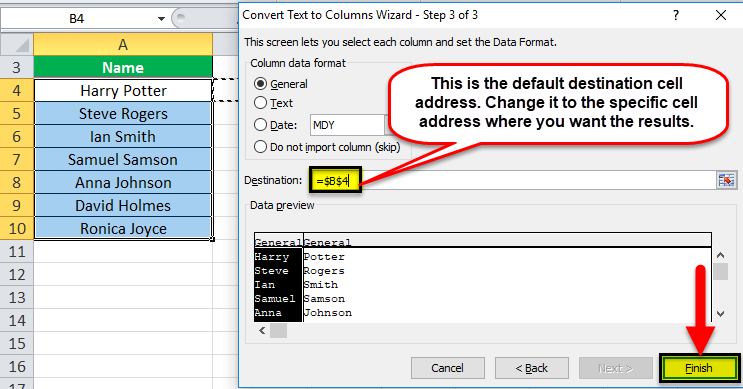
Under “destination,” specify the cell in which the output is required. Enter “$B$4” and click “finish.”

Note: If you proceed with the default cell address under “destination,” the output will replace the original dataset. To retain the initial data as is, select a cell to its right as the “destination.”

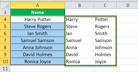
The output is shown in the following image. The names of column A have been split into the first name (column B) and the last name (column C).

Note: The results of the “text to columns” property are static. This means that any change made to the source data is not reflected in the results. Hence, to include the changes, the whole process has to be repeated.

Example #2–Split by “Fixed Width” Option

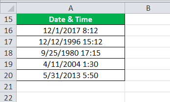
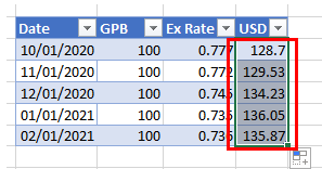
The following list shows the date and time of specific days. We want to split the date and time into separate columns. Use the “fixed width” option of the text to columns wizard.

Step 1: Select the range A16:A20, as shown in the following image. In the Data tab, click “text to columns” under the “data tools” group.

Step 2: The “convert text to columns wizard” dialog box appears. Select the option “fixed width,” as shown in the following image. Click “next.”

Step 3: Under “data preview,” place a break line (on the text) at the position where splitting is to be carried out.

Since we want to split the date and time, we insert the break line between these two data strings. Click “next.”

Note: To remove the break line, double-click on it.

Step 4: Under “column data format,” select date, as shown in the following image. In “destination,” enter the cell address where the results are required. Click “finish.”

Step 5: The output is shown in the following image. The data strings of column A have been split into the dates (column B) and the time (column C).

Frequently Asked Questions

When a cell is split, its components are divided into separate cells. Splitting is often done when there is a need to sort and re-arrange the existing data. Since the substrings of data are moved to new cells, splitting helps to analyze the resulting columns.

To split an excel cell, the text to columns feature is used. This separates the data of a cell, based on either the delimiter character or the fixed length of a substring.

The steps to split cell in excel are listed as follows:
a. Select the cells to be divided. In the Data tab, click “text to columns” under the “data tools” group.
b. Select the option “delimited” or “fixed width.” Click “next.”
c. If “delimited” is selected, enter the required separator in “delimiters.” If “fixed width” is selected, insert the break line at the desired position.
d. Select the “column data format” and specify the “destination.” Click “finish.”

The content of the selected cells is split into different excel columns.

Let us split column A which consists of data strings separated by a comma and space.

The entries in the range A1:A5 are listed as follows:
• Jack Adams, Chicago, USA, 2016
• Peter Smith, Houston, USA, 2019
• Ella Taylor, Glasgow, UK, 2018
• Lily Brown, Birmingham, UK, 2015
• Birdie Evans, Paris, France, 2020

The steps to split data into multiple cells using the “delimited” option are stated as follows:

a. In the Data tab, select the option “text to columns.” This is under the “data tools” group.
b. The “convert text to columns wizard” dialog box appears. Select “delimited” under “choose the file type that best describes your data.” Click “next.”
c. Select the checkboxes for both comma and space. Select the checkbox for “treat consecutive delimiters as one.” Click “next.”
d. Select “general” under the “column data format.” Enter “$B$1” under “destination.” Click “finish.”

Five separate columns (columns B to F) are created containing the first names, last names, cities, countries, and years respectively.

Note 1: Before the procedure begins, ensure that there are empty columns to the right of the destination cell. This prevents overwriting the source data.

Note 2: It is recommended to glance through the “data preview” before clicking “finish” in the last step. This ensures that the splitting of data is executed properly.

The flash fill feature helps to split cells automatically. When the user enters the split up text in a few cells one by one, Excel senses a pattern and fills the remaining cells.

Let us split the first and the last names of column A containing Jack Adams, Peter Smith, Ella Taylor, Lily Brown, and Birdie Evans (in the range A1:A5).

The steps of splitting excel cells with the help of flash fill are listed as follows:

a. In column B, enter the first name “Jack” in cell B1.
b. Enter “Peter” in the subsequent cell B2.
c. Excel detects a pattern and displays the first names for the remaining cells B3, B4, and B5. Press the “Enter” key.

Column B is filled with the first names (in the range B1:B5).

Note 1: Ensure that the first names in cells B1 and B2 are entered without the double quotation marks.

Note 2: Alternatively, after the first step (step a), click “flash fill” under the “data tools” group of the Data tab. This populates similar data in the remaining cells.

How to divide numbers and cells in Microsoft Excel to make calculations and analyze data

Twitter LinkedIn icon The word «in».

LinkedIn Fliboard icon A stylized letter F.

Flipboard Facebook Icon The letter F.

Email Link icon An image of a chain link. It symobilizes a website link url.

You can divide in Excel using a few different methods.
It’s easy to divide two numbers or cell values in Excel using the forward slash in a simple formula.
You can also divide a column of values by a constant, using the dollar sign to create an absolute reference in your spreadsheet.
Visit Business Insider’s homepage for more stories.

There are a few common techniques for performing division in Excel.

You can divide numbers directly in a single cell, or use a simple formula to divide the contents of two different cells. You can also set up a formula that divides a series of values by a constant.

Here’s what you need to know to divide in Excel on a Mac or PC.

Check out the products mentioned in this article:

MacBook Pro (From $1,299.99 at Best Buy)

Lenovo IdeaPad 130 (From $299.99 at Best Buy)

How to divide two numbers in Excel

You can divide two numbers using the forward slash (/) in a formula.

If you type «=10/5» in a cell and press Enter on the keyboard, you should see the cell display «2.»

You can also divide the values stored in different cells.

1. In a cell, type «=».

2. Click in the cell that contains the dividend (the dividend is the number on the top of a division calculation).

3. Type «/».

4. Click the second cell that contains the divisor.

5. Press Enter.

How to divide a column of values by a constant

It’s not uncommon to need to divide a column of numbers by a constant. You can do that by using an absolute reference to the cell that contains the constant divisor.

1. Create a column of numbers that will serve as the dividend in your division calculations. Then put the constant divisor in another cell.

2. In a new cell, type «=» and click the first cell in your list of dividends.

3. Type the name of the cell that contains the divisor, adding a «$» before both the letter and number. Using the dollar sign in this way turns the reference into an absolute reference, so it won’t change when you paste it elsewhere in the spreadsheet.

4. Press Enter.

5. Copy and paste this result to other cells to do more division on the other dividends. You can drag the cell by its lower right corner to copy it down a column.

Источник

See all How-To Articles

This tutorial will demonstrate how to divide cells and columns in Excel and Google Sheets.

The Divide Symbol

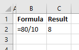
The divide symbol in Excel is the forward slash on the keyboard (/). This is the same as using the division sign (÷) in mathematics. When you divide two numbers in Excel, start with an equal sign (=), which will create a formula. Then type in the first number (the number you want to divide), followed by the forward slash, and then the number you wish to divide by.

=80/10

The result of this formula would then be 8.

Divide With a Cell Reference and a Constant

For greater flexibility in your formula, use the reference of a cell as the number to be divided and a constant as the number to divide by.

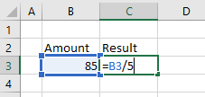
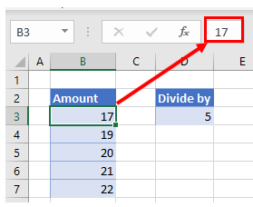
To divide B3 by 5, type the formula:

=B3/5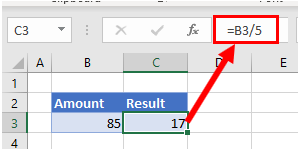

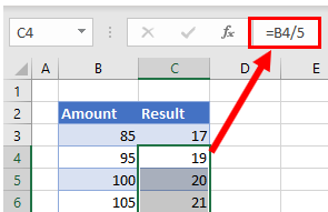
Then copy this formula down the column to the rows below. The constant number (5) will remain the same but the cell address for each row will change according to the row you are in due to Relative Cell referencing.

Divide a Column With Cell References

You can also use a cell reference for the number to divide by.

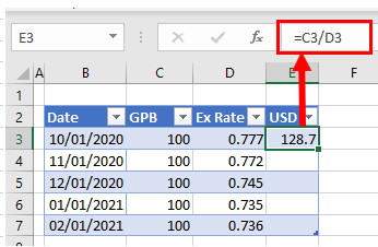
To divide cell C3 by cell D3, type the formula:

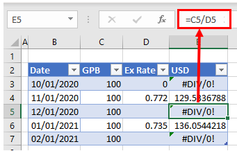
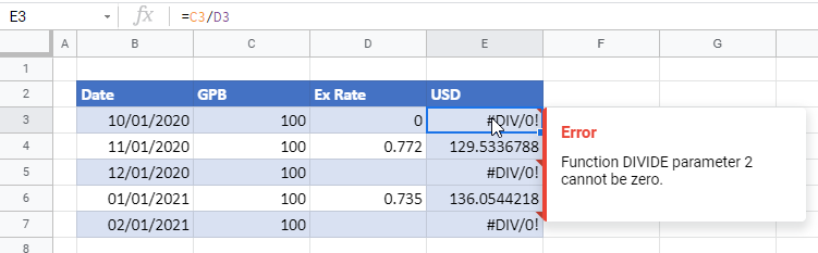
=C3/D3

Since the formula uses cell addresses, you can then copy this formula down to the rest of the rows in the table.

As the formula uses Relative Cell addresses, the formula will change according to the row it is copied down to.

Note: that you can also divide numbers in Excel by using the QUOTIENT Function.

Divide a Column With Paste Special

You can divide a column of numbers by a divisor, and return the result as a number within the same cell.

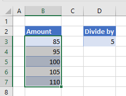
Select the divisor (in this case, 5) and in the Ribbon, go to Home > Copy, or press CTRL + C.

Highlight the cells to be divided (in this case B3:B7).

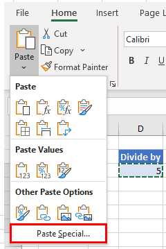
In the Ribbon, go to Home > Paste > Paste Special.

In the Paste Special dialog box, select Divide and then click OK.

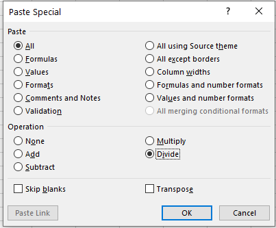
The values in the highlighted cells will be divided by the divisor that was copied and the result will be returned in the same location as the highlighted cells. In other words, you will overwrite your original values with the new divided values; cell references are not used in this this method of calculation.

The #DIV/0! Error

If you try and divide a number by zero, you will get an error as there is no answer when a number is divided by zero.

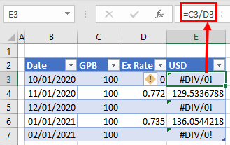
You will also get an error if you try and divide a number by a blank cell.

To prevent this from happening, you can use the IFERROR Function in your formula.

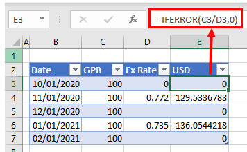
Using the methods above, you can also add, subtract, or multiply cells and columns in Excel.

How to Divide Cells and Columns in Google Sheets

Apart from the divide Paste Special function (which does not work in Google Sheets), all of the above examples will work in exactly the same way in Google Sheets.

Источник

We are used to working with whole excel cells within columns and rows. At times, you find yourself working with data imported from other sources or even working with data that is not in the format you are used to. Such data can appear in one cell alone (especially when working with texts with limited commas). Most beginners using Microsoft Excel spreadsheets may not be aware that it is possible to split a cell into two or multiple smaller ones to solve such a dilemma. Unfortunately, I do not mean to split one cell into two or numerous cells figuratively. By dividing cells in Excel, we suggest adding a new column, changing the column widths, and merging two cells into one.

Splitting excels cells helps provide better sorting and filtering features for your data. Using the Unmerge Cells, Text to Column feature, and Flash Fill features, you will be able to split Excel cells. In this article, we learn how to separate Excel cells using different methods. Let’s get started.

Method 1: splitting cells using the Delimiter with Text to Column feature

1. In an open Excel workbook, click and select all the cells you want to split.

2. from the main menu ribbon, click on the Data tab.

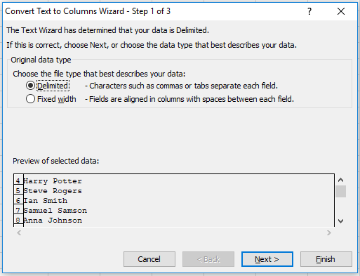
3. Under the Data Tools tab, select the ‘Text to Columns’ option to display the ‘Convert Text to Columns Wizard – Step 1 to 3’ dialog box.

4. In the dialog box, for step 1, check on the ‘Delimited’ option checkbox. Click Next to proceed.

5. Under the’ Delimiters’ section, step 2 of the wizard dialog box, specify the delimiter you want to split. You will be able to see a preview of any applied delimiters you select in the ‘Data preview’ field. Click Next to proceed.

6. In the 3^rd step, select a Destination for your selected cells data.

7. Click Finish. Every text or value string in that cell will split into different cells.

Method 2: splitting cells using VBA macro

1. In this example, I will split the cells with the following sentences using VBA macro

1. Go to the Developers tab and click on the ‘Visual Basic’ option or (Press Alt+F11 to access the visual basic editor)

2. The ‘Visual Basic Editor’ window will be displayed.

3. Click on the Insert tab. From the given options, select Module to create a new module

4. Type in VBA code into the ‘Code Window.’

Public Sub SplitName()

X = Cells(Rows.Count, 1).End(xlUp).Row

For A = 1 To X

B = InStr(Cells(A, 1), » «)

C = InStrRev(Cells(A, 1), » «)

Cells(A, 2) = Left(Cells(A, 1), B)

Cells(A, 3) = Mid(Cells(A, 1), B, C – B)

Cells(A, 4) = Right(Cells(A, 1), Len(Cells(A, 1)) – C)

Next A

End Sub

5. Click the Run tab and select Run Macro to display a dialog box. (Or simply press F5 to run the code)

6. In the ‘Macro’ dialog box, click the Run button.

Method 3: using the flash fill feature

1. In your open workbook, select empty cell columns right beside the main column you want to split.

2. In the first cell of the first column, type in the first value or text you want to split and press Enter.

3. Type the second name in the second cell. Flash fill feature will appear. If not Go to the Data tab on the main ribbon, click on the Flash Fill option indicating the cell you had typed in. you will see that the first part (all values or texts) in the main column has been split automatically in the adjacent column.

4. Carry on the process for the other columns to separate all text or value strings.

Method 4: splitting cells by using the unmerge cells option in Excel.

While working on imported Excel files, you may find the data merged, or some cells are combined. An easy way to split these cells is by clicking on the Unmerge Cells options. To do this;

1. In your open workbook, select all the cells you need to split.

2. In the Home tab, under the Alignment group, click on the Merge & Centre drop-down arrow.

3. Select Unmerge Cells, and this will divide your merged cells.

Conclusion

The article below gives you different methods on how to split or divide cells. As a constant Excel user who comes across cells you need to separate, you can select either of the methods above to achieve this.

Источник

Содержание

Разъединение ячеек
- Способ 1: окно форматирования
- Способ 2: кнопка на ленте
Вопросы и ответы

Одной из интересных и полезных функций в Экселе является возможность объединить две и более ячейки в одну. Эта возможность особенно востребована при создании заголовков и шапок таблицы. Хотя, иногда она используется даже внутри таблицы. В то же время, нужно учесть, что при объединении элементов некоторые функции перестают корректно работать, например сортировка. Также существует и много других причин, из-за которых пользователь решит разъединить ячейки, чтобы построить структуру таблицы по-иному. Установим, какими методами можно это сделать.

Разъединение ячеек

Процедура разъединения ячеек является обратной их объединению. Поэтому, говоря простыми словами, чтобы её совершить, нужно произвести отмену тех действий, которые были выполнены при объединении. Главное понять, что разъединить можно только ту ячейку, которая состоит из нескольких ранее объединенных элементов.

Способ 1: окно форматирования

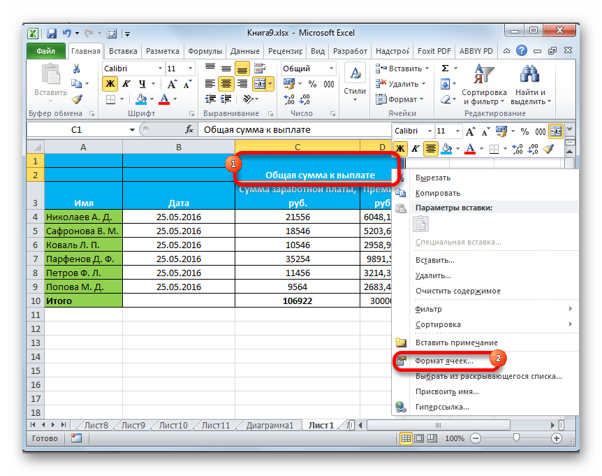
Большинство пользователей привыкли производить процесс объединения в окне форматирования с переходом туда через контекстное меню. Следовательно, и разъединять они будут так же.

Выделяем объединенную ячейку. Щелкаем правой кнопкой мышки для вызова контекстного меню. В списке, который откроется, выбираем пункт «Формат ячеек…». Вместо этих действий после выделения элемента можно просто набрать комбинацию кнопок на клавиатуре Ctrl+1.

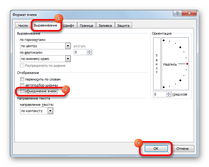
После этого запускается окно форматирования данных. Перемещаемся во вкладку «Выравнивание». В блоке настроек «Отображение» снимаем галочку с параметра «Объединение ячеек». Чтобы применить действие, щелкаем по кнопке «OK» внизу окна.

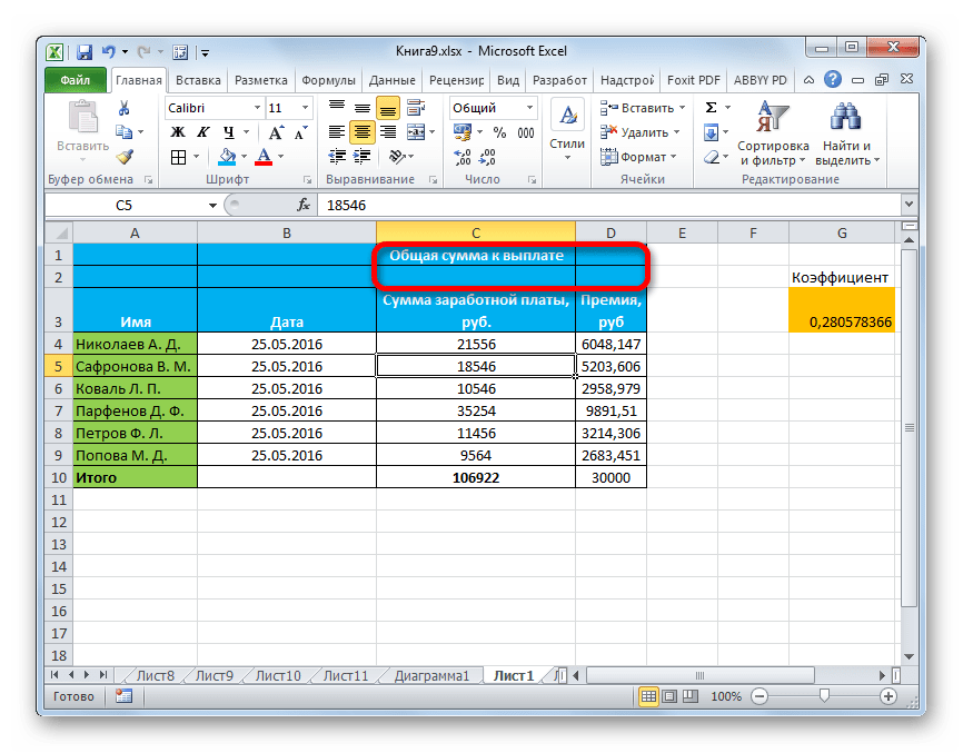
После этих несложных действий ячейка, над которой проводили операцию, будет разделена на составляющие её элементы. При этом, если в ней хранились данные, то все они окажутся в верхнем левом элементе.

Урок: Форматирование таблиц в Экселе

Способ 2: кнопка на ленте

Но намного быстрее и проще, буквально в один клик, можно произвести разъединение элементов через кнопку на ленте.

Как и в предыдущем способе, прежде всего, нужно выделить объединенную ячейку. Затем в группе инструментов «Выравнивание» на ленте жмем на кнопку «Объединить и поместить в центре».

В данном случае, несмотря на название, после нажатия кнопки произойдет как раз обратное действие: элементы будут разъединены.

Собственно на этом все варианты разъединения ячеек и заканчиваются. Как видим, их всего два: окно форматирования и кнопка на ленте. Но и этих способов вполне хватает для быстрого и удобного совершения вышеуказанной процедуры.

Еще статьи по данной теме:

Помогла ли Вам статья?

Источник

Looking to learn how to divide in Microsoft Excel? You’ve come to the right place.

In this article I’ll cover:

How to divide in a cell
How to divide cells
How to divide a range of cells by a constant number
How to use the QUOTIENT function

How to divide in Excel shortcut

To divide in Excel you’ll need to write your formula with the arithmetic operator for division, the slash symbol (/).

You can do this three ways: with the values themselves, with the cell references, or using the QUOTIENT function.

Ex. =20/10, =A2/A3, =QUOTIENT(A2,A3)

Related: Be sure to check out how to multiply in Excel, how to subtract in Excel, and how to add in Excel!

If you’re looking to learn how to divide in Excel, you’ll need to know how to write Excel formulas.

Excel formulas are expressions used to display values that are calculated from the data you’ve entered and they’re generally used to perform various mathematical, statistical, and logical operations.

So before we jump into the specifics of how to divide in Excel, here are a few reminders to keep in mind when writing Excel formulas:

All Excel formulas should begin with the equal sign (=). This is a must in order for Excel to recognize it as a formula.
The cells will display the result of the formula, not the actual formula. So by using cell references rather than just entering the data in the cell, if you need to go back later the values will be easier to understand.
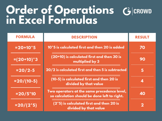
When using arithmetic operators in your formula, remember the order of operations (I personally reference the acronym PEMDAS: Parenthesis, Exponentiation, Multiplication, Division, Addition, Subtraction.) Below you’ll find an example of how the order of operations is applied to formulas in Excel.

How to divide in a cell

To divide numbers in a cell, you’ll need to write your formula in the designated cell. Your formula should start with the equal sign (=), and contain the arithmetic operator (/) needed for the calculation. In this case, you want to divide 20 by 2, so your formula is =20/2.

Once you’ve entered the formula, press ‘Enter’ and your result will populate. In this example, the division formula, =20/2, yields a result of 10 (see below).

How to divide cells

To divide cells, the data will need to be in its own cells so that you can use the cell references in the formula.

You can see below that a division formula was written in cell C1 using cell references, but the data had to be entered separately in cells A1 and B3.

Once you’ve entered the formula, press ‘Enter’ and your result will populate. In this example, the division formula, =A1/B3, yields a result of 5 (see below).

How to divide a range of cells by a constant number

Want to divide each cell in a range by a constant number? By writing your formula with the dollar sign symbol ($), you’re telling Excel that the reference to the cell is “absolute,” meaning when you copy the formula to different cells, the reference will always be to that cell. In this example, cell C2 is absolute.

That being said, to divide each cell in column A by the constant number in C2, start by writing your formula as you would if you were dividing cells, but add ‘$’ in front of the column letter and row number. In this case, your formula is =A2/$C$2.

Next, drag the formula to the other cells in the range. This copies the formula to the new cells, updating the data, but keeping the constant.

The results will populate as you drag and drop the formula (see below).

How to use the QUOTIENT function

With division, sometimes results will have a remainder. For example, if you enter the multiplication formula =10/6 in Excel, your result would be 1.6667.

The QUOTIENT function, though, will only return the integer portion of a division – not the remainder. Therefore, you should use this function if you want to discard of the remainder.

To use this function, navigate to the ‘Formulas’ tab and click ‘Insert Function’ or start typing ‘=QUOTIENT’ in the cell you want the result to populate in. Select ‘QUOTIENT.’

From there, enter your cell references (or numbers) in the function. Be sure to separate the cell references with a comma (,).

Press ‘Enter’ and the integer result – without the remainder – will populate. So, rather than =10/6 equaling 1.6667, using the QUOTIENT function yields 1.

You’re ready to divide in Excel!

And that’s it! In this article, we’ve covered everything you need to know about how to divide in Excel using formulas and functions.

Now grab your computer and dive into Excel to give it a try for yourself!

Did you enjoy this article? Check out our articles on how merge cells in Excel and how to lock cells in Excel!

Jordan Wahl is a former content manager at G2. She holds a BBA in Marketing from the University of Wisconsin-Whitewater. She loves anything that puts her in her creative space. including writing, art, and music.

Источник

In Excel, you can divide in a cell, cells, columns of cells, a range of cells by a constant number, and by using the QUOTIENT function.

In Excel, you can divide within a cell, cell by cell, columns of cells, range of cells by a constant number, and divide using QUOTIENT function.

Dividing using Divide symbol in a cell

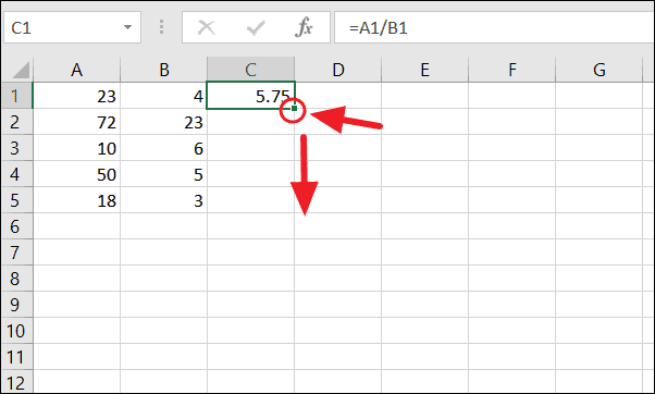
The easiest method to divide numbers in excel is by using the divide operator. In MS Excel, the divide operator is a forward slash (/).

To divide numbers in a cell, simply, start a formula with the ‘=’ sign in a cell, then enter the dividend, followed by a forward slash, followed by the divisor.

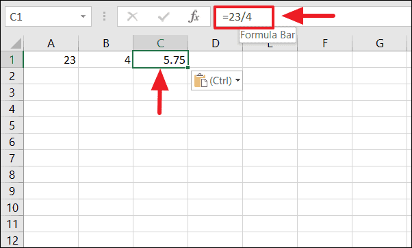
=number/number

For example, to divide 23 by 4, you type this formula in a cell: =23/4

Dividing Cells in Excel

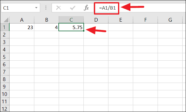
To divide two cells in Excel, enter the equals sign (=) in a cell, followed by two cell references with the division symbol in between. For example, to divide the cell value A1 by B1, type ‘=A1/B1’ in cell C1.

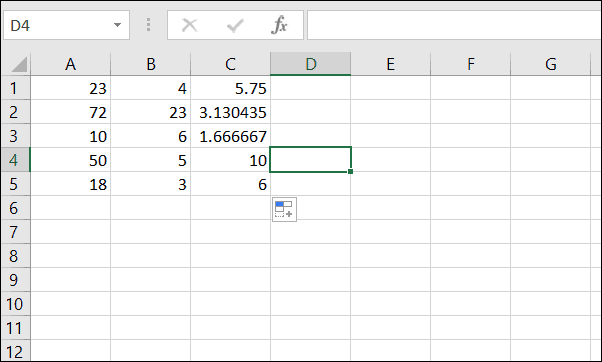
Dividing Columns of Cells in Excel

To divide two columns of numbers in Excel, you can use the same formula. After you, typed the formula in the first cell (C1 in our case), click on the small green square in the lower-right corner of cell C1 and drag it down to cell C5.

Now, the formula is copied from C1 to C5 of column C. And column A is divided by column B, and the answers were populated in column C.

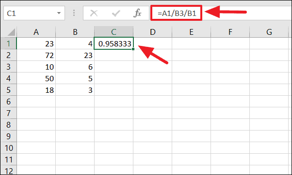
For example, to divide the number in A1 by the number in B2, and then divide the result by the number in B1, use the formula in the following image.

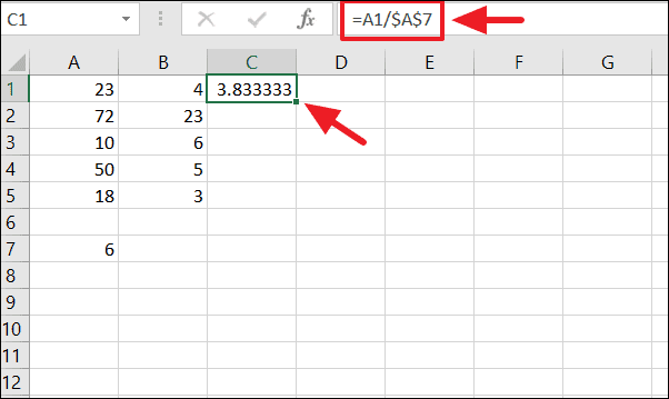
Dividing a Range of Cells by a Constant Number in Excel

If you want to divide a range of cells in a column by a constant number, you can do that by fixing the reference to the cell that contains the constant number by adding the dollar ‘$’ symbol in front of the column and row in the cell reference. This way, you can lock that cell reference so it won’t change no matter where the formula is copied.

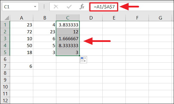
For example, we created an absolute cell reference by placing a $ symbol in front of the column letter and row number of cell A7 ($A$7). First, enter the formula in cell C1 to divide the value of cell A1 by the value of cell A7.

To divide a range of cells by a constant number, click on the small green square in the lower-right corner of cell C1 and drag it down to cell C5. Now, the formula is applied to C1:C5 and cell C7 is divided by a range of cells (A1:A5).

Divide a Column by the Constant Number with Paste Special

You can also divide a range of cells by the same number with Paste Special method. To do that, right-click on the cell A7 and copy (or press CTRL + c).

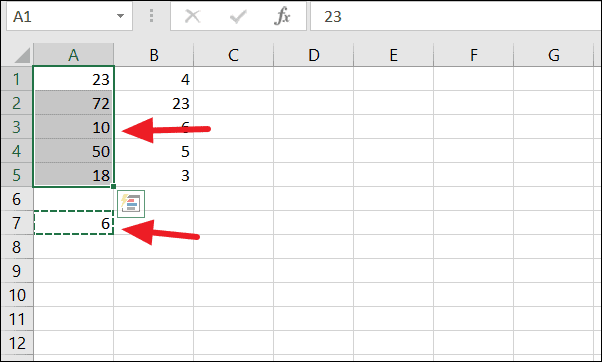
Next, select the cell range A1:A5 and then right-click, and click ‘Paste Special’.

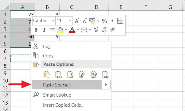
Select ‘Divide’ under ‘Operations’ and click the ‘OK’ button.

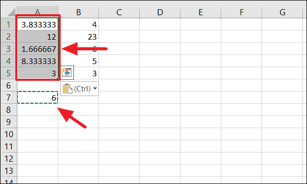
Now, cell A7 is divided by the column of numbers (A1:A5). But the original cell values of A1:A5 will be replaced with the results.

Dividing in Excel using QUOTIENT Function

Another way to divide in Excel is by using the QUOTIENT function. However, dividing numbers of cells using the QUOTIENT returns only the integer number of a division. This function discards the remainder of a division.

The Syntax for QUOTIENT function:

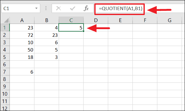
=QUOTIENT(numerator, denominator)

When you divide two numbers evenly without remainder, the QUOTIENT function returns the same output as the division operator.

For example, both =50/5 and =QUOTIENT(50, 5) yields 10.

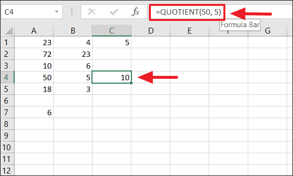
But, when you divide two numbers with a remainder, the divide symbol produces a decimal number while the QUOTIENT returns only the integer part of the number.

For example, =A1/B1 returns 5.75 and =QUOTIENT(A1,B1) returns 5.

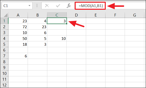
If you only want the remainder of a division, not an integer, then use the Excel MOD function.

For example, =MOD(A1,B1) or =MOD(23/4) returns 3.

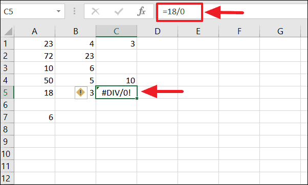
#DIV/O! Error

#DIV/O! error value is one of the most common errors associated with division operations in Excel. This error will be displayed when the denominator is 0 or the cell reference is incorrect.

We hope this post helps you divide in Excel.

Источник

Split the content from one cell into two or more cells

See Also

Need more help?

Want more options?

Introduction to Divide Cell in Excel

Examples of Divide Cell in Excel

Example #1 – Divide cells with Delimiter in Excel

Example #2 – Divide cells with Fixed Width in Excel

Things to Remember

Recommended Articles

How do you divide cells?

How do I divide a whole number in Excel?

What is the formula of division?

How do I multiply two columns in Excel?

Is there a divide function in Excel?

How do I split a group of numbers in Excel?

How do you show a number divided by 1000 in Excel?

How do I split a column into two parts in Excel?

How do you divide by 1000?

How do you multiply in Excel formula?

How do you equally space cells in sheets?

How do I split a cell into multiple rows?

How do you add and divide cells in Excel?

How do I split a whole column in sheets?

What is the shortcut to divide in Excel?

Distribute the contents of a cell into adjacent columns

Need more help?

Split Cells in Excel

Table of contents

How to Split a Cell in Excel?

Example #1–Split by “Delimited” Option

Example #2–Split by “Fixed Width” Option

Frequently Asked Questions

Recommended Articles

How to divide numbers and cells in Microsoft Excel to make calculations and analyze data

Check out the products mentioned in this article:

MacBook Pro (From $1,299.99 at Best Buy)

Lenovo IdeaPad 130 (From $299.99 at Best Buy)

How to divide two numbers in Excel

How to divide a column of values by a constant

The Divide Symbol

Divide With a Cell Reference and a Constant

Divide a Column With Cell References

Divide a Column With Paste Special

The #DIV/0! Error

How to Divide Cells and Columns in Google Sheets

Method 1: splitting cells using the Delimiter with Text to Column feature

Method 2: splitting cells using VBA macro

Method 3: using the flash fill feature

Method 4: splitting cells by using the unmerge cells option in Excel.

Conclusion

Разъединение ячеек

Способ 1: окно форматирования

Способ 2: кнопка на ленте

Еще статьи по данной теме:

Помогла ли Вам статья?

How to divide in Excel shortcut

How to divide in a cell

How to divide cells

How to divide a range of cells by a constant number

How to use the QUOTIENT function

Dividing using Divide symbol in a cell

Dividing Cells in Excel

Dividing Columns of Cells in Excel

Dividing a Range of Cells by a Constant Number in Excel

Divide a Column by the Constant Number with Paste Special

Dividing in Excel using QUOTIENT Function

#DIV/O! Error