How do you cut text in excel - Word и Excel - помощь в работе с программами

In this tutorial I will describe the functions used to cut pieces of text — LEFT, RIGHT, and MID.

Excel is a powerful spreadsheet program that is widely used in various industries for data management, analysis, and reporting. One of the common tasks in Excel is cutting text, which means removing a portion of text from a cell or string of text. Cutting text can be useful for cleaning up data, separating information into different cells, or extracting specific information from a larger dataset.

How to cut text?

In this article, we will explore different methods to cut text in Excel, including using the Cut command, LEFT, RIGHT, and MID functions. These techniques will help you save time and improve the accuracy of your data analysis and reporting.

In all of the features listed below the text argument, unless it is a reference to a cell or the formula returns the text must be enclosed in quotes!

Formulas to cut text

If you want to cut a certain number of characters from the beginning of a cell, you can use the LEFT function. LEFT function allows you to cut the text portion of the specified length, starting from the beginning (left side). Its syntax is as follows:

LEFT (text; [num_chars])

Type «=LEFT(cell reference, number of characters)» into the formula bar, replacing «cell reference» with the cell containing the text and «number of characters» with the number of characters you want to cut.

If you want to cut a certain number of characters from the end of a cell, you can use the RIGHT function. RIGHT function allows you to cut out the text of a given length from the end of the text (from right). Its syntax is as follows:

RIGHT (text; [num_chars])

Type «=RIGHT(cell reference, number of characters)» into the formula bar, replacing «cell reference» with the cell containing the text and «number of characters» with the number of characters you want to cut.

For both functions num_chars argument is optional. When you ignore it, it will be downloaded by default only one character of text — the first in the event of the LEFT function, the last in the RIGHT function. If num_chars will be greater than the length of the text, the functions return the entire text.

If you want to cut a certain number of characters from the middle of a cell, you can use the MID function. To display a certain number of characters from text starting at a specific location allows MID function. Here’s the syntax:

MID (text; start_num; [num_chars])

start_num is the place from where we want to start cutting operations.

Type «=MID(cell reference, starting position, number of characters)» into the formula bar, replacing «cell reference» with the cell containing the text, «starting position» with the position in the text where you want to start cutting, and «number of characters» with the number of characters you want to cut.

For example, to start from the beginning of the text, type 1 (position of the first character). The argument here num_chars works the same way as in the previous two functions — if the argument start_num total more than the entire text, the function returns characters from the specified position to the end of the text. The following illustration shows how to use the function:

Cutting Pieces of Text After Particular Sign

In this example you will teach yourself how to cut a piece of text after some particular sign.

Sometimes it happens that you receive some strange data. There are some part which you don’t need and it is hard to get rid of them. In this example you have data which begins with product code. Content which you need is after coma (,) sign.

There is a way in Excel to extract substrings. Just use this formula for: =MID(A2,FIND(«,»,A2)+1,LEN(A2)-FIND(«,»,A2)+1)

Paste this formula to your cell to extract data from A1 cell. Drag and drop down to extract data from another cells in A column.

Different formula I know is =TRIM(MID(A2,FIND(«,»,A2,1)+1,100))

It works the same way. There is another proof that you can do the same things in different ways within Excel.

Источник

Cutting Data To cut data, select the cell or cells you want to cut and use the keyboard shortcut “Ctrl+X” (hold down the “Ctrl” key and the “X” key at the same time).

Contents

1 Can you clip cells in Excel?
2 How do I shorten a text string in Excel?
3 How do you clip data in Excel?
4 How do you isolate a cell in Excel?
5 How do I shorten text in a cell?
6 How do I cut text left in Excel?
7 How do I clip text in Excel 2020?
8 How do you make a long sentence in one cell in Excel?
9 How do I put a footer in Excel?
10 How do you select certain cells in Excel?
11 How do I return just the numbers in a cell?
12 How do you select a range of cells in Excel without dragging?
13 How do I remove 3 letters from a cell in Excel?
14 How do you trim the first character in Excel?
15 How do I remove a left and right character in Excel?
16 What is wrapped text in Excel?
17 Which option fits text in the cell?
18 How do I keep text in one cell in Excel without wrapping it?
19 How do I make a list in one cell in Excel?
20 How do I make multiple lines in one cell in Excel?

Can you clip cells in Excel?

In Excel, adjust the column to the required width, then enable word-warp on that column (which will cause all row heights to increase) and then finally select all rows and adjust row heights to the desired height. Voila!

How do I shorten a text string in Excel?

The formula is “=DIRECTION(Cell Name, Number of characters to display)” without the quotation marks. For example: =LEFT(A3, 6) displays the first six characters in cell A3. If the text in A3 says “Cats are better”, the truncated text will read “Cats a” in your selected cell.

How do you clip data in Excel?

Wrap text in a cell

Select the cells.
On the Home tab, click Wrap Text. The text in the selected cell wraps to fit the column width. When you change the column width, text wrapping adjusts automatically. Note: If all wrapped text is not visible, it might be because the row is set to a specific height.

How do you isolate a cell in Excel?

Place your mouse pointer on “Highlight Cell Rules” and review the list of options. Choose the one most appropriate for your purpose and click on it to open the rules dialog box. For example, select “equal to” to isolate a specific value or “duplicate values” to find duplicate data entries.

How do I shorten text in a cell?

How to truncate text in Excel – Excelchat

Step 1: Prepare your data sheet.
Step 2: Select cell/column where you want the truncated text string to appear.
Step 3: Type the RIGHT or LEFT truncating formula in the target cell.

How do I cut text left in Excel?

Remove characters from left side of a cell

=REPLACE(old_text, start_num, num_chars, new_text)
=RIGHT(text,[num_chars])
=LEN(text)

How do I clip text in Excel 2020?

On the Home tab, in the Alignment group, click Wrap Text. (On Excel for desktop, you can also select the cell, and then press Alt + H + W.) Notes: Data in the cell wraps to fit the column width, so if you change the column width, data wrapping adjusts automatically.

How do you make a long sentence in one cell in Excel?

Here is how I do it:

Widen the column where the text is to be displayed to a reasonable width.
Select the cell (or the entire column if you’re going to type lots of text throughout the column)
Right-click on the selection.
Choose “Format Cells”
Click on the Alignment tab.
Check the “Wrap text” box.
Click OK.

On the Insert tab, in the Text group, click Header & Footer. Excel displays the worksheet in Page Layout view. To add or edit a header or footer, click the left, center, or right header or footer text box at the top or the bottom of the worksheet page (under Header, or above Footer). Type the new header or footer text.

How do you select certain cells in Excel?

Select one or more cells

Click on a cell to select it. Or use the keyboard to navigate to it and select it.
To select a range, select a cell, then with the left mouse button pressed, drag over the other cells.
To select non-adjacent cells and cell ranges, hold Ctrl and select the cells.

How do I return just the numbers in a cell?

Extracting Numbers from the Right of a Text or Number String by Combining RIGHT, LEN, MIN & SEARCH Functions. Press Enter & then use Fill Handle to autofill the rest of the cells. MIN function is used to find the lowest digit or number from an array.

How do you select a range of cells in Excel without dragging?

Select a Large Range of Cells With the Shift Key
Click the first cell in the range you want to select. Scroll your sheet until you find the last cell in the range you want to select. Hold down your Shift key, and then click that cell. All the cells in the range are now selected.

How do I remove 3 letters from a cell in Excel?

1) In Number text, type the number of characters you want to remove from the strings, here I will remove 3 characters. 2) Check Specify option, then type the number which you want to remove string start from in beside textbox in Position section, here I will remove characters from third character.

How do you trim the first character in Excel?

1. Combine RIGHT and LEN to Remove the First Character from the Value. Using a combination of RIGHT and LEN is the most suitable way to remove the first character from a cell or from a text string. This formula simply skips the first character from the text provided and returns the rest of the characters.

How do I remove a left and right character in Excel?

In Excel 2013 and later versions, there is one more easy way to delete the first and last characters in Excel – the Flash Fill feature. In a cell adjacent to the first cell with the original data, type the desired result omitting the first or last character from the original string, and press Enter.

What is wrapped text in Excel?

“Wrapping text” means displaying the cell contents on multiple lines, rather than one long line. This will allow you to avoid the “truncated column” effect, make the text easier to read and better fit for printing. In addition, it will help you keep the column width consistent throughout the entire worksheet.

Which option fits text in the cell?

In “Table Tools” click the [Layout] tab > locate the “Cell Size” group and choose from of the following options: To fit the columns to the text (or page margins if cells are empty), click [AutoFit] > select “AutoFit Contents.”

How do I keep text in one cell in Excel without wrapping it?

If you want to hide the overflow text in a cell, such as A1 in this example, without having to type anything into the adjacent cells, right-click on the cell and select “Format Cells” from the popup menu. On the “Format Cells” dialog box, click the “Alignment” tab. Select “Fill” from the “Horizontal” drop-down list.

How do I make a list in one cell in Excel?

To have the entire list in a single Excel cell:

Select the list in your word processor.
Press Ctrl + C to copy it.
Go to Excel > double-click your cell.
Press Ctrl + V to paste the list. The list will appear in a single cell.

How do I make multiple lines in one cell in Excel?

You can put multiple lines in a cell with pressing Alt + Enter keys simultaneously while entering texts. Pressing the Alt + Enter keys simultaneously helps you separate texts with different lines in one cell. With this shortcut key, you can split the cell contents into multiple lines at any position as you need.

Источник

Загрузить PDF

Данная статья научит вас обрезать текст в Microsoft Excel. Для этого вам в первую очередь потребуется ввести в Excel полные неукороченные данные.

1

Запустите Microsoft Excel. Если у вас уже создан документ с данными, которые требуют обработки, дважды кликните по нему мышкой, чтобы открыть. В ином случае вам необходимо запустить Microsoft Excel, чтобы создать новую книгу и ввести в нее данные.
2
Выделите ячейку, в которой должен быть выведен укороченный текст. Это необходимо сделать тогда, когда в книгу у вас уже введены необработанные данные.
- Обратите внимание, что выбранная ячейка должна отличаться от той ячейки, в которой содержится полный текст.
3
Введите формулу ЛЕВСИМВ или ПРАВСИМВ в выделенную ячейку. Принцип действия формул ЛЕВСИМВ и ПРАВСИМВ одинаков, несмотря на то, что ЛЕВСИМВ отражает заданное количество символов от начала текста заданной ячейки, а ПРАВСИМВ – от ее конца. Вводимая вами формула должна выглядеть следующим образом: «=ЛЕВСИМВ(адрес ячейки с текстом; количество символов для отображения)». Кавычки вводить не нужно. Ниже приведено несколько примеров использования упомянутых функций.^[1]
- Формула =ЛЕВСИМВ(A3;6) покажет первые шесть символов текста из ячейки A3. Если в исходной ячейке содержится фраза «кошки лучше», то в ячейке с формулой появится укороченная фраза «кошки».
- Формула =ПРАВСИМВ(B2;5) покажет последние пять символов текста из ячейки B2. Если в ячейке B2 содержится фраза «я люблю wikiHow», то в ячейке с формулой появится укороченный текст «kiHow».
- Помните о том, что пробелы в тексте тоже считаются за символ.
4

Когда закончите ввод параметров формулы, нажмите на клавиатуре клавишу Enter. Ячейка с формулой автоматически отразит обрезанный текст.

Реклама

1
Выделите ячейку, в которой должен появиться обрезанный текст. Эта ячейка должна отличаться от той ячейки, в которой содержится обрабатываемый текст.
- Если вы еще не ввели данные для обработки, то это нужно сделать в первую очередь.
2
Введите формулу ПСТР в выделенную ячейку. Функция ПСТР позволяет извлечь текст из середины строки. Вводимая формула должна выглядеть следующим образом: «=ПСТР(адрес ячейки с текстом, порядковый номер начального символа извлекаемого текста, количество извлекаемых символов)». Кавычки вводить не нужно. Ниже приведено несколько примеров.
- Формула =ПСТР(A1;3;3) отражает три символа из ячейки A1, первый из которых занимает третью позицию от начала полного текста. Если в ячейке A1 содержится фраза «гоночный автомобиль», то в ячейке с формулой появится сокращенный текст «ноч».
- Аналогичным образом, формула =ПСТР(B3;4;8) отражает восемь символов из ячейки B3, начиная с четвертой позиции от начала текста. Если в ячейке B3 содержится фраза «бананы – не люди», то в ячейке с формулой появится сокращенный текст «аны – не».
3

Когда закончите ввод параметров формулы, нажмите на клавиатуре клавишу Enter. Ячейка с формулой автоматически отразит обрезанный текст.

Реклама

1

Выберите ячейку с текстом, которую вы хотите разбить. В ней должно содержаться больше текстовых символов, чем пробелов.
2

Нажмите на вкладку Данные. Она расположена вверху на панели инструментов.
3
Нажмите на кнопку Текст по столбцам. Эта кнопка расположена на панели инструментов в группе кнопок под названием «Работа с данными».
- С помощью функциональных возможностей данной кнопки можно поделить содержимое ячейки Excel на несколько отдельных колонок.
4

В появившемся окне настроек активируйте опцию фиксированной ширины. После нажатия на предыдущем шаге кнопки Текст по столбцам откроется окно настроек с названием «Мастер текстов (разбор) – шаг 1 из 3». В окне у вас будет возможность выбора одной из двух опций: «с разделителями» или «фиксированной ширины». Опция «с разделителями» подразумевает, что текст будет разделен на части по пробелам или запятым. Данная опция обычно бывает полезна при обработке данных, импортированных из других приложений и баз данных. Опция «фиксированной ширины» позволяет создать из текста колонки с заданным количеством текстовых символов.
5

Нажмите кнопку Далее. Перед вами появится описание трех возможных вариантов действий. Чтобы вставить конец строки текста, щелкните в нужной позиции. Чтобы удалить конец строки, дважды щелкните по разделительной линии. Чтобы переместить конец строки, нажмите на разделительную линию и перетащите ее в нужное место.
6

Снова нажмите кнопку Далее. В данном окне вам также предложат несколько опций формата данных столбца на выбор: «общий», «текстовый», «дата» и «пропустить столбец». Просто пропустите данную страницу, если только вы не хотите намеренно поменять исходный формат своих данных.
7

Нажмите на кнопку Готово. Теперь исходный текст будет разделен на две или более отдельных ячеек.

Реклама

Об этой статье

Эту страницу просматривали 127 764 раза.

Была ли эта статья полезной?

Источник

Содержание

How to Split Text in Excel (5 Easy Ways To Separate Text)
Using Text to Columns
Using TRIM Function to Trim Extra Spaces
Using Formula To Separate Text in Excel
Split String with Delimiter
Split String at Specific Character
Using Flash Fill
Using VBA Function
Subscribe and be a part of our 15,000+ member family!

How to Split Text in Excel (5 Easy Ways To Separate Text)

One scenario is where you need to join multiple strings of text into a single text string. The flip of that is splitting a single text string into multiple text strings. If the data at hand was copied from somewhere or created by someone who completely missed the point of Excel columns, you will find that you need to split a block of text to categorize it.

Splitting the text largely depends on the delimiter in the text string. A delimiter is a character or symbol that marks the beginning or end of a character string. Examples of a delimiter are a space character, hyphen, period, comma.

Our example case for this guide involves splitting book details into book title, author, and genre. The delimiter we’ve used is a comma:

This tutorial will teach you how to split text in Excel with the Text to Columns and Flash Fill features, formulas, and VBA. The formulas method includes splitting text by a specific character. That’s the menu today.

Let’s get splitting!

Table of Contents

Using Text to Columns

This feature lives up to its name. Text to Columns splits a column of text into multiple columns with specified controls. Text to Columns can split text with delimiters and since our data contains only a comma as the delimiter, using the feature becomes very easy. See the following steps to split text using Text to Columns:

Select the data you want to split.
Go to the Data tab and select the Text to Columns icon from the Data Tools

Select the Delimited radio button and then click on the Next

In the Delimiters section, select the Comma
Then select the Next button.

Now you need to choose where you want the split text. Click on the Destination field, then select the destination cell on the worksheet in the background where you want the split text to start.
Select the Finish button to close the Text to Columns

Using the comma delimiter to separate the text string, Text to Columns has split the text from our example case into three columns:

Luckily, our data doesn’t contain a book with commas in the book name. If we had the book Cows, Pigs, Wars and Witches by Marvin Harris in the dataset, the text would be split into 5 columns instead of 3 like the rest. If the delimiter in your data is appearing in the text string for more than delimiting, you’ll have better luck splitting text with other methods. Now unto another observation.

Let’s cast a closer look at the output of Text to Columns. Notice how the last two columns carry one leading space? You can see that the values in columns D and E are not a hundred percent aligned to the left:

The last two columns carry a leading space because Text to Columns only takes the delimiter as a mark from where to split the text. The space character after the comma is carried with the next unit of text and that has our data with a leading space.

A quick fix for this is to use the TRIM function to clear up extra spaces. Here is the formula we have used to remove leading spaces from columns D and E:

The TRIM function removes all spaces from a text string other than a single space character between two words. Any leading, trailing, or extra spaces will be removed from the cell’s value. We have simply used the formula with a reference of the cell containing the leading space.

And that cleaned up the leading spaces for us. Data – good to go!

Using Formula To Separate Text in Excel

We can make use to Excel functions to construct formulas that can help us in splitting a text string into multiple.

Split String with Delimiter

Using a formula can also split a single text string into multiple strings but it will require a combo of functions. Let’s have a little briefing on the functions that make part of this formula we will use for splitting text.

The SUBSTITUTE function replaces old text in a text string with new text.

The REPT function repeats text a given number of times.

The LEN function returns the number of characters in a text string.

The MID function returns a given number of characters from the middle of a text string with a specified starting position.

The TRIM function removes all spaces, other than single spaces between words, from a text string.

Now let’s see how these functions combined can be used to split text with a single formula:

In our example, the first cell we are using this formula on is cell B5. The number of characters in B5 as counted by the LEN function is 49. The REPT function repeats spaces (denoted by “ “ in the formula) in B5 for the number of characters supplied by the LEN function i.e. 49.

The SUBSTITUTE function replaces the commas “,” in B5 with 49 space characters supplied by the REPT function. Since there are two commas in B5, one after the book name and one after the author, 49 spaces will be entered after the book name and 49 spaces after the author, creating a decent gap between the text we want to split.

Now let’s see the calculations for the MID function. The first bit is (C$4-1). In row 4, we added serial numbering for each of the columns for our categories. The row has been locked in the formula with a $ sign so the row doesn’t change as the formula is copied down. But we have left the column free so that the serial number changes for the respective columns used in the formula.

In the formula, 1 is subtracted from C4 (1-1=0) and the result is multiplied by the number of characters in B5 i.e. LEN($B5) and then 1 is added to the expression. The calculation for the starting position in the MID function, i.e. (C$4-1)*LEN($B5)+1, becomes (1-1)*49+1 which equals 1.

The MID function returns the text from the middle of B5, the starting position is 1 (that means the text to be returned is to start from the first character) and the number of characters to be returned is LEN($B5) i.e 49 characters. Since we have added 49 spaces in place of each of the commas, that gives us plenty of area to safely return just one chunk of text along with some extra spaces. The result up until the MID function is A Song of Ice and Fire with lots of trailing spaces.

The extra spaces are no problem. The TRIM function cleans any extra spaces leaving the single spaces between words and so we finally have the book name returned as A Song of Ice and Fire.

Now for the next column and hence the next category, the calculation for the starting position in the MID function will change like so (D$4-1)*LEN($B5)+1. The expression comes down to (2-1)*49+1 which equals 50. If the MID function is to return characters starting from the 50th character, with all the extra spaces added by the REPT function, what the MID function will return will be along this pattern: spaces author spaces.

The leading and trailing spaces will be trimmed by the TRIM function and the result will be George RR Martin.

The “+1” in the starting position argument of the MID function has no relevance for the subsequent columns, only for the first. That is because, without the “+1” in the first column’s calculation, it would be 0*49 which will end up in a #VALUE! error.

The formula copied along column E gives us the genre from the combined text in column B and that completes our set.

Split String at Specific Character

If there is only a single delimiter that is a specific character, such a lengthy formula as above will not be required to split the text. Let’s say, like our case example below, we are to split product code and product type which is joined by a hyphen.

Now this would be easier if the product code had a fixed number of characters; we would only have to use the LEFT function to return a certain number of characters. But what’s the fun in that?

We are going to let the FIND function do a bit of search work for us and find the hyphen in the text so the LEFT function and RIGHT function can return the surrounding text. This is the formula with the LEFT function for returning the first extract:

The FIND function searches B3 for the position of the hyphen “-“ in the text string, which is 6. The LEFT function then returns the characters starting from the left of the text and the number of characters to return is 6-1. “-1” at the end ensures that the characters returned do not include the hyphen itself. Here are the results of this formula for returning the first segment of split text:

Now for the second segment of text, the RIGHT function comes into play with this formula:

The FIND function is again used to find the location of the hyphen in B3 which we know is the 6th character. The LEN function returns the number of characters in B3 as 23. The RIGHT function extracts 23-6 characters from B3 and returns the product type “Bluetooth Speaker”. This is how it has worked for our example:

Using Flash Fill

The Flash Fill feature in Excel automatically fills in values based on a couple of manually provided examples. The ease of Flash Fill is that you need not remember any formulas, use any wizards, or fiddle with any settings. If your data is consistent, Flash Fill will be the quickest to pick up on what you are trying to get done. Let’s see the steps for using Flash Fill to split text and how it works for our example case:

Type the first text as an example for Flash Fill to pick up the pattern and press the Enter

From the Home tab’s Editing group, click on the Fill icon and select Flash Fill from the menu.
Alternatively, use the shortcut keys Ctrl + E.

Picking up on the provided example, Flash Fill will split the text and fill the column according to the same pattern:

Repeat the same steps for each column to be Flash-Filled.

Flash Fill will save the trouble of having to trim leading and trailing spaces but as mentioned, if there are any anomalies or inconsistencies in the data (e.g a space before and after the comma), Flash Fill won’t be a reliable method of splitting text and due to the bulk of the data, the problem may go ignored. If you doubt the data to have inconsistencies, use the other methods for splitting the text.

Using VBA Function

The final method we will be discussing today for splitting text will be a VBA function. In order to automate tasks in MS Office applications, macros can be created and used with VBA. Our task is to split text in Excel and below are the steps for doing this using VBA:

If you have the Developer tab added to the toolbar Ribbon, click on the Developer tab and then select the Visual Basic icon in the Code group to launch the Visual Basic
You can also use the Alt + F11 keys.

The Visual Basic editor will have opened:

Open the Insert tab and select Module from the list. A Module window will open.

In the Module window, copy-paste the following code to create a macro titled SplitText:

Edit the following parts of the code as per your data:

‘For n = 4 To 16’ – 4 and 16 represent the first and last rows of the dataset.
‘MyArray = Split(Cells(n, 2), «,»)’ – The comma enclosed with double quotes is the delimiter.
‘Count = 3’ – 3 is the column number of the first column that the resulting data will be returned in.

To run the code, press the F5

The data will be split as per the supplied values:

Clean up the leading spaces in columns D and E using the TRIM function:

Now let’s split the active guide from its conclusion. Today you learned a few ways on how to split text in Excel. If you find yourself splitting hairs on your ability to split text next time, pocket this one and be ready to give it a go! We’ll be back with more Excel-ness to fill your pockets. Make some space!

Subscribe and be a part of our 15,000+ member family!

Now subscribe to Excel Trick and get a free copy of our ebook «200+ Excel Shortcuts» (printable format) to catapult your productivity.

Источник

MID function in Excel is intended to select a substring from a string of text passed as the first argument, and returns the required number of characters starting from the specified position.

Examples of using the MID function in Excel

One character in single-byte-encoded languages corresponds to 1 byte. When working with such languages, the results of the functions MID and MIDB (returns a substring from a string based on the number of specified bytes) do not differ. If a two-byte language is used on the computer, each character will be counted as two characters when using MIDB. The two-byte languages are Korean, Japanese, and Chinese.

How to divide the text into several cells in columns in Excel?

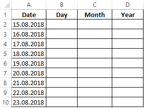
Example 1. The table column contains dates recorded as text strings. Record separately in adjacent columns the number of the day, month and year, isolated from the presented dates.

View source data table:

To fill in the day number, use the following formula:

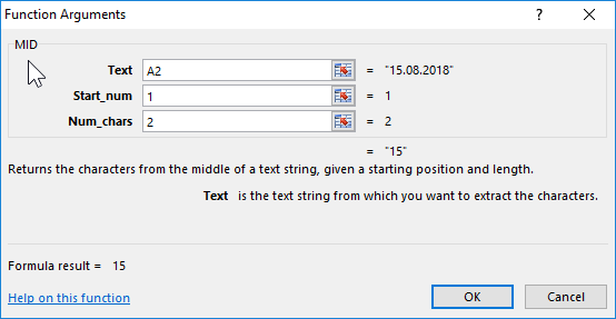
Argument Description:

A2:A10 — a range of cells with a textual representation of the dates from which the numbers of the days will be highlighted;
1 — the number of the initial position of the character of the extracted substring (the first character in the original string);
2 — the number of the last position of the character of the extracted substring.

In a similar way, we select the month numbers and years to fill in the corresponding columns, taking into account that the month number starts with the 4th character in each row and the year from the 7th. We use the following formulas:

=MID(A2:A10,4,2)

=MID(A2:A10,7,4)

View of the completed data table:

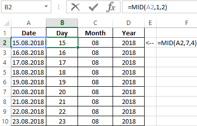
Thus, we were able to cut the text into cells of column A. It was possible to divide each date separately into several cells by columns: day, month, and year.

How to cut part of cell text in Excel?

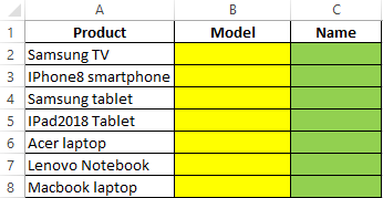
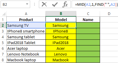
Example 2. A text column with the name and brand of goods is stored in a table column. Split the existing lines into substrings with the name and brand, respectively, and write the values in the corresponding columns of the table.

View of data table:

To fill the column «Name» we use the following formula:

=MID(A2,1,FIND(«»,A2))

FIND function returns the position number of the space character «» in the line being scanned, which is taken as an argument to the number_ characters of the MID function. As a result of the calculations we get:

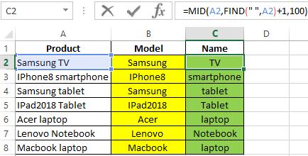
To fill the “Mark” column, use the following array formula:

=MID(A2:A8,FIND(«»,A2:A8)+1,100)

FIND function returns the position of the space character. A unit is added to the received number to find the position of the first character of the brand name of the product. The final value is used as an argument to the Start_num of the MID function. For simplicity, instead of searching for the last position number (for example, using the LEN function), the number 100 is indicated, which in this example is guaranteed to exceed the number of characters in the original line.

As a result of the calculations we get:

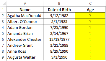
How to calculate age by date of birth in Excel?

Example 3. The table contains information about employees in the columns name and date of birth. Create a column in which the surname of the employee and his age in the format “Jon — 27” will be displayed.

View source table:

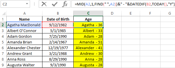
To return a string with the last name and current age, use the following formula:

MID function returns part of a string to a space character, whose position is determined by the FIND function. To find the age of the employee, use the DATEDIF function, the resulting value of which is truncated to the nearest smaller integer to get the number of full years. The TEXT function converts the resulting value to a text string.

For connection (concatenation) of the obtained strings the symbols “&” are used. As a result of the calculations we get:

Features of using the MID function in Excel

The function has the following syntax entry:

=MID(Text,Start_num,Num_chars)

Argument Description:

Text – a required argument that accepts a cell reference with a text or a text string enclosed in quotes from which a substring of a certain length will be extracted starting from the specified position of the first character;
Start_num – is a required argument that accepts integers from the range from 1 to N, where N is the length of the string from which you want to extract a substring of a given size. The initial position of the character in the string corresponds to the number 1. If this argument takes a fractional number from the range of valid values, the fractional part will be truncated;
Num_chars – is a required argument that takes a value from a range of non-negative numbers, which characterizes the length in characters of the returned substring. If the argument is the number 0 (zero), the MID function returns an empty string. If the argument is a number greater than the number of characters in the string, the entire part of the string starting with the specified second position argument will be returned. In fractional numbers used as the argument, the fractional part is truncated.

MIDB function has a similar syntax:

=MIDB(Text,Start_num,Num_bytes)

It has a single argument:

Num_bytes is a required argument that accepts integers from the range from 1 to N, where N is the bytes in the source string, characterizing the number of bytes in the returned substring.

Download examples MID function for splitting text in Excel

Notes:

MID function will return an empty string if, as an argument, the Start_num was passed value exceeding the number of characters in the source string.
If the value 1 was passed as an argument for Start_num, and Num_chars argument is determined by a number that is equal to or greater than the total number of characters in the source line, the MID function returns the entire line.
If the argument Start_num was specified by a number from the range of negative numbers or 0 (by zero), the MID function will return the error code #VALUE!.
If the Num_chars argument is a negative number, the result of the MID function is the error code #VALUE!.

Источник

Our example case for this guide involves splitting book details into book title, author, and genre. The delimiter we’ve used is a comma:

Let’s get splitting!

Using Text to Columns

Select the data you want to split.
Go to the Data tab and select the Text to Columns icon from the Data Tools

Select the Delimited radio button and then click on the Next

In the Delimiters section, select the Comma
Then select the Next button.

Now you need to choose where you want the split text. Click on the Destination field, then select the destination cell on the worksheet in the background where you want the split text to start.
Select the Finish button to close the Text to Columns

Using the comma delimiter to separate the text string, Text to Columns has split the text from our example case into three columns:

Using TRIM Function to Trim Extra Spaces

A quick fix for this is to use the TRIM function to clear up extra spaces. Here is the formula we have used to remove leading spaces from columns D and E:

=TRIM(C4)

And that cleaned up the leading spaces for us. Data – good to go!

Using Formula To Separate Text in Excel

We can make use to Excel functions to construct formulas that can help us in splitting a text string into multiple.

Split String with Delimiter

The SUBSTITUTE function replaces old text in a text string with new text.

The REPT function repeats text a given number of times.

The LEN function returns the number of characters in a text string.

The MID function returns a given number of characters from the middle of a text string with a specified starting position.

The TRIM function removes all spaces, other than single spaces between words, from a text string.

Now let’s see how these functions combined can be used to split text with a single formula:

=TRIM(MID(SUBSTITUTE($B5,",",REPT(" ",LEN($B5))),(C$4-1)*LEN($B5)+1,LEN($B5)))

The extra spaces are no problem. The TRIM function cleans any extra spaces leaving the single spaces between words and so we finally have the book name returned as A Song of Ice and Fire.

The leading and trailing spaces will be trimmed by the TRIM function and the result will be George RR Martin.

The formula copied along column E gives us the genre from the combined text in column B and that completes our set.

Split String at Specific Character

Now this would be easier if the product code had a fixed number of characters; we would only have to use the LEFT function to return a certain number of characters. But what’s the fun in that?

=LEFT(B3,FIND("-",B3)-1)

Now for the second segment of text, the RIGHT function comes into play with this formula:

=RIGHT(B3,LEN(B3)-FIND("-",B3))

Using Flash Fill

Type the first text as an example for Flash Fill to pick up the pattern and press the Enter

From the Home tab’s Editing group, click on the Fill icon and select Flash Fill from the menu.
Alternatively, use the shortcut keys Ctrl + E.

Picking up on the provided example, Flash Fill will split the text and fill the column according to the same pattern:

Repeat the same steps for each column to be Flash-Filled.

Using VBA Function

If you have the Developer tab added to the toolbar Ribbon, click on the Developer tab and then select the Visual Basic icon in the Code group to launch the Visual Basic
You can also use the Alt + F11 keys.

The Visual Basic editor will have opened:

Open the Insert tab and select Module from the list. A Module window will open.

In the Module window, copy-paste the following code to create a macro titled SplitText:

Sub SplitText()
Dim MyArray() As String, Count As Long, i As Variant
For n = 4 To 16
 MyArray = Split(Cells(n, 2), ",")
 Count = 3
 For Each i In MyArray
 Cells(n, Count) = i
 Count = Count + 1
 Next i
Next n
End Sub

Edit the following parts of the code as per your data:

‘For n = 4 To 16’ – 4 and 16 represent the first and last rows of the dataset.
‘MyArray = Split(Cells(n, 2), «,»)’ – The comma enclosed with double quotes is the delimiter.
‘Count = 3’ – 3 is the column number of the first column that the resulting data will be returned in.

To run the code, press the F5

The data will be split as per the supplied values:

Clean up the leading spaces in columns D and E using the TRIM function:

Источник

When you are reading a WPS excel file, you’ve probably noticed that there is a lot of extra content in the top and bottom of the columns. This can be very annoying when you’re trying to access a specific column or row on your spreadsheet. Cutting off text in Excel is one of the most common actions — whether you’re extracting a part of a cell, or want to create a table from your data. There are different ways to do it and in this tutorial we’ll show you how to remove this excess info and make reading your spreadsheets much more easier.

How to cut off text in excel using LEFT function?

This method works best with versions 2016/2016/mac/online.

There are a lot of reasons you might need to cut off text in excel, from managing large chunks of data to cutting off names and addresses for privacy when you’re transferring an entire spreadsheet to another person. Either way, the most common function used to cut off text is the LEFT() function. And here’s how you can use it.

1. To truncate characters, first select the data in a worksheet. If you have a spreadsheet with the data, you can simply double-click on it to open. But if you do not have it, then you will have to enter it into a sheet. Once you have the data in a worksheet, you can use Excel’s built-in functions to truncate characters.

2. In the next step, you will create a cell with the truncated text string. If you are truncating text for an entire column, then you will also have to prepare a whole column to display the truncated text.

3. To truncate text strings, type the LEFT formula into the cell where you want your first result to appear.

The syntax of the formula is given as follows:

=LEFT (A1,3)

Where;

A1 refers to the target cell, and 3 refers to how many characters after the cell’s contents will remain.

How to cut off text in excel using RIGHT function?

This method works best with versions 2016/2016/mac/online

We can use RIGHT function as well to cut off text in excel. And here’s how it is used.

1. RIGHT function works the same way as LEFT function does to cut off text in excel but when we use this function, only the last characters will be displayed.

2. For example, the following formula would produce the similar result:

=RIGHT(A1,3)

3. As mentioned above, this function would display characters from the right side of the cell.

How to hide the overflow text in excel?

This method works best with versions 2016/2016/mac/online

1. First of all, select the cell or range of cells for which you want to hide the overflow text.

2. After selecting the cells, press CTRL+1 and select Fill option from Horizontal drop down menu under the Alignment section.

3. Once you select the fill option and hit OK, the overflow text will hide.

Did you learn about how to cut off text in excel? You can follow WPS Academy to learn more features of Word Document, Excel Spreadsheets and PowerPoint Slides.

You can also download WPS Office to edit the word documents, excel, PowerPoint for free of cost. Download now! And get an easy and enjoyable working experience.

Источник

Split text into different columns with functions

Excel for Microsoft 365 Excel for Microsoft 365 for Mac Excel for the web Excel 2021 Excel 2021 for Mac Excel 2019 Excel 2019 for Mac Excel 2016 Excel 2016 for Mac Excel 2013 Excel Web App Excel 2010 Excel 2007 Excel for Mac 2011 More…Less

You can use the LEFT, MID, RIGHT, SEARCH, and LEN text functions to manipulate strings of text in your data. For example, you can distribute the first, middle, and last names from a single cell into three separate columns.

The key to distributing name components with text functions is the position of each character within a text string. The positions of the spaces within the text string are also important because they indicate the beginning or end of name components in a string.

For example, in a cell that contains only a first and last name, the last name begins after the first instance of a space. Some names in your list may contain a middle name, in which case, the last name begins after the second instance of a space.

This article shows you how to extract various components from a variety of name formats using these handy functions. You can also split text into different columns with the Convert Text to Columns Wizard

	Example name	Description	First name	Middle name	Last name	Suffix
1	Jeff Smith	No middle name	Jeff		Smith
2	Eric S. Kurjan	One middle initial	Eric	S.	Kurjan
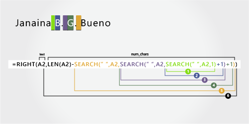
3	Janaina B. G. Bueno	Two middle initials	Janaina	B. G.	Bueno
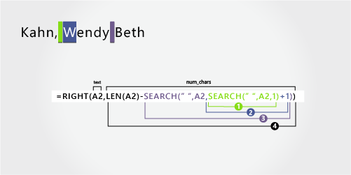
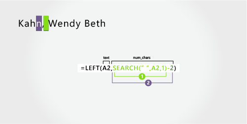
4	Kahn, Wendy Beth	Last name first, with comma	Wendy	Beth	Kahn
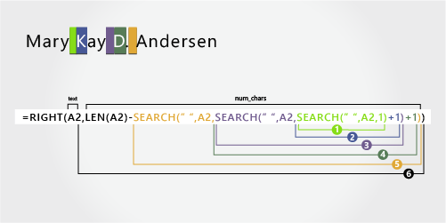
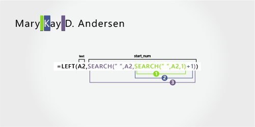
5	Mary Kay D. Andersen	Two-part first name	Mary Kay	D.	Andersen
6	Paula Barreto de Mattos	Three-part last name	Paula		Barreto de Mattos
7	James van Eaton	Two-part last name	James		van Eaton
8	Bacon Jr., Dan K.	Last name and suffix first, with comma	Dan	K.	Bacon	Jr.
9	Gary Altman III	With suffix	Gary		Altman	III
10	Mr. Ryan Ihrig	With prefix	Ryan		Ihrig
11	Julie Taft-Rider	Hyphenated last name	Julie		Taft-Rider

Note: In the graphics in the following examples, the highlight in the full name shows the character that the matching SEARCH formula is looking for.

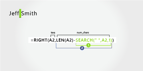
This example separates two components: first name and last name. A single space separates the two names.

Copy the cells in the table and paste into an Excel worksheet at cell A1. The formula you see on the left will be displayed for reference, while Excel will automatically convert the formula on the right into the appropriate result.

Hint Before you paste the data into the worksheet, set the column widths of columns A and B to 250.

Example name	Description
Jeff Smith	No middle name
Formula	Result (first name)
‘=LEFT(A2, SEARCH(» «,A2,1))	=LEFT(A2, SEARCH(» «,A2,1))
Formula	Result (last name)
‘=RIGHT(A2,LEN(A2)-SEARCH(» «,A2,1))	=RIGHT(A2,LEN(A2)-SEARCH(» «,A2,1))

First name

The first name starts with the first character in the string (J) and ends at the fifth character (the space). The formula returns five characters in cell A2, starting from the left.

Use the SEARCH function to find the value for num_chars:

Search for the numeric position of the space in A2, starting from the left.
Last name

The last name starts at the space, five characters from the right, and ends at the last character on the right (h). The formula extracts five characters in A2, starting from the right.

Use the SEARCH and LEN functions to find the value for num_chars:

Search for the numeric position of the space in A2, starting from the left. (5)
Count the total length of the text string, and then subtract the number of characters to the left of the first space, as found in step 1.

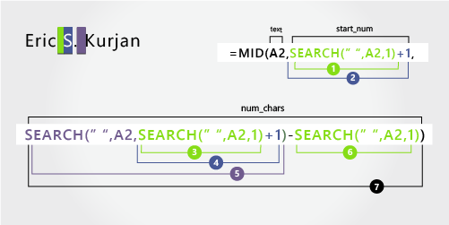
This example uses a first name, middle initial, and last name. A space separates each name component.

Hint Before you paste the data into the worksheet, set the column widths of columns A and B to 250.

Example name	Description
Eric S. Kurjan	One middle initial
Formula	Result (first name)
‘=LEFT(A2, SEARCH(» «,A2,1))	=LEFT(A2, SEARCH(» «,A2,1))
Formula	Result (middle initial)
‘=MID(A2,SEARCH(» «,A2,1)+1,SEARCH(» «,A2,SEARCH(» «,A2,1)+1)-SEARCH(» «,A2,1))	=MID(A2,SEARCH(» «,A2,1)+1,SEARCH(» «,A2,SEARCH(» «,A2,1)+1)-SEARCH(» «,A2,1))
Formula	Live Result (last name)
‘=RIGHT(A2,LEN(A2)-SEARCH(» «,A2,SEARCH(» «,A2,1)+1))	=RIGHT(A2,LEN(A2)-SEARCH(» «,A2,SEARCH(» «,A2,1)+1))

First name

The first name starts with the first character from the left (E) and ends at the fifth character (the first space). The formula extracts the first five characters in A2, starting from the left.

Use the SEARCH function to find the value for num_chars:

Search for the numeric position of the space in A2, starting from the left. (5)
Middle name

The middle name starts at the sixth character position (S), and ends at the eighth position (the second space). This formula involves nesting SEARCH functions to find the second instance of a space.

The formula extracts three characters, starting from the sixth position.

Use the SEARCH function to find the value for start_num:

Search for the numeric position of the first space in A2, starting from the first character from the left. (5).
Add 1 to get the position of the character after the first space (S). This numeric position is the starting position of the middle name. (5 + 1 = 6)

Use nested SEARCH functions to find the value for num_chars:

Search for the numeric position of the first space in A2, starting from the first character from the left. (5)
Add 1 to get the position of the character after the first space (S). The result is the character number at which you want to start searching for the second instance of space. (5 + 1 = 6)
Search for the second instance of space in A2, starting from the sixth position (S) found in step 4. This character number is the ending position of the middle name. (8)
Search for the numeric position of space in A2, starting from the first character from the left. (5)
Take the character number of the second space found in step 5 and subtract the character number of the first space found in step 6. The result is the number of characters MID extracts from the text string starting at the sixth position found in step 2. (8 – 5 = 3)
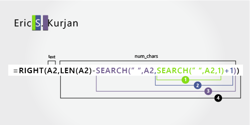
Last name

The last name starts six characters from the right (K) and ends at the first character from the right (n). This formula involves nesting SEARCH functions to find the second and third instances of a space (which are at the fifth and eighth positions from the left).

The formula extracts six characters in A2, starting from the right.
Use the LEN and nested SEARCH functions to find the value for num_chars:

Search for the numeric position of space in A2, starting from the first character from the left. (5)
Add 1 to get the position of the character after the first space (S). The result is the character number at which you want to start searching for the second instance of space. (5 + 1 = 6)
Search for the second instance of space in A2, starting from the sixth position (S) found in step 2. This character number is the ending position of the middle name. (8)
Count the total length of the text string in A2, and then subtract the number of characters from the left up to the second instance of space found in step 3. The result is the number of characters to be extracted from the right of the full name. (14 – 8 = 6).

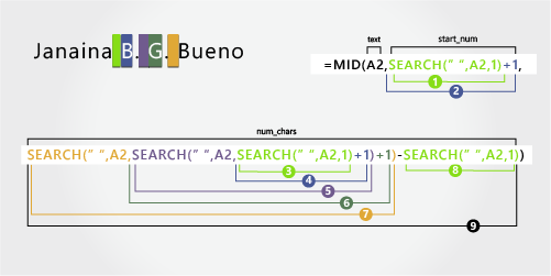
Here’s an example of how to extract two middle initials. The first and third instances of space separate the name components.

Hint Before you paste the data into the worksheet, set the column widths of columns A and B to 250.

Example name	Description
Janaina B. G. Bueno	Two middle initials
Formula	Result (first name)
‘=LEFT(A2, SEARCH(» «,A2,1))	=LEFT(A2, SEARCH(» «,A2,1))
Formula	Result (middle initials)
‘=MID(A2,SEARCH(» «,A2,1)+1,SEARCH(» «,A2,SEARCH(» «,A2,SEARCH(» «,A2,1)+1)+1)-SEARCH(» «,A2,1))	=MID(A2,SEARCH(» «,A2,1)+1,SEARCH(» «,A2,SEARCH(» «,A2,SEARCH(» «,A2,1)+1)+1)-SEARCH(» «,A2,1))
Formula	Live Result (last name)
‘=RIGHT(A2,LEN(A2)-SEARCH(» «,A2,SEARCH(» «,A2,SEARCH(» «,A2,1)+1)+1))	=RIGHT(A2,LEN(A2)-SEARCH(» «,A2,SEARCH(» «,A2,SEARCH(» «,A2,1)+1)+1))

First name

The first name starts with the first character from the left (J) and ends at the eighth character (the first space). The formula extracts the first eight characters in A2, starting from the left.

Use the SEARCH function to find the value for num_chars:

Search for the numeric position of the first space in A2, starting from the left. (8)
Middle name

The middle name starts at the ninth position (B), and ends at the fourteenth position (the third space). This formula involves nesting SEARCH to find the first, second, and third instances of space in the eighth, eleventh, and fourteenth positions.

The formula extracts five characters, starting from the ninth position.

Use the SEARCH function to find the value for start_num:

Search for the numeric position of the first space in A2, starting from the first character from the left. (8)
Add 1 to get the position of the character after the first space (B). This numeric position is the starting position of the middle name. (8 + 1 = 9)

Use nested SEARCH functions to find the value for num_chars:

Search for the numeric position of the first space in A2, starting from the first character from the left. (8)
Add 1 to get the position of the character after the first space (B). The result is the character number at which you want to start searching for the second instance of space. (8 + 1 = 9)
Search for the second space in A2, starting from the ninth position (B) found in step 4. (11).
Add 1 to get the position of the character after the second space (G). This character number is the starting position at which you want to start searching for the third space. (11 + 1 = 12)
Search for the third space in A2, starting at the twelfth position found in step 6. (14)
Search for the numeric position of the first space in A2. (8)
Take the character number of the third space found in step 7 and subtract the character number of the first space found in step 6. The result is the number of characters MID extracts from the text string starting at the ninth position found in step 2.
Last name

The last name starts five characters from the right (B) and ends at the first character from the right (o). This formula involves nesting SEARCH to find the first, second, and third instances of space.

The formula extracts five characters in A2, starting from the right of the full name.

Use nested SEARCH and the LEN functions to find the value for the num_chars:

Search for the numeric position of the first space in A2, starting from the first character from the left. (8)
Add 1 to get the position of the character after the first space (B). The result is the character number at which you want to start searching for the second instance of space. (8 + 1 = 9)
Search for the second space in A2, starting from the ninth position (B) found in step 2. (11)
Add 1 to get the position of the character after the second space (G). This character number is the starting position at which you want to start searching for the third instance of space. (11 + 1 = 12)
Search for the third space in A2, starting at the twelfth position (G) found in step 6. (14)
Count the total length of the text string in A2, and then subtract the number of characters from the left up to the third space found in step 5. The result is the number of characters to be extracted from the right of the full name. (19 — 14 = 5)

In this example, the last name comes before the first, and the middle name appears at the end. The comma marks the end of the last name, and a space separates each name component.

Hint Before you paste the data into the worksheet, set the column widths of columns A and B to 250.

Example name	Description
Kahn, Wendy Beth	Last name first, with comma
Formula	Result (first name)
‘=MID(A2,SEARCH(» «,A2,1)+1,SEARCH(» «,A2,SEARCH(» «,A2,1)+1)-SEARCH(» «,A2,1))	=MID(A2,SEARCH(» «,A2,1)+1,SEARCH(» «,A2,SEARCH(» «,A2,1)+1)-SEARCH(» «,A2,1))
Formula	Result (middle name)
‘=RIGHT(A2,LEN(A2)-SEARCH(» «,A2,SEARCH(» «,A2,1)+1))	=RIGHT(A2,LEN(A2)-SEARCH(» «,A2,SEARCH(» «,A2,1)+1))
Formula	Live Result (last name)
‘=LEFT(A2, SEARCH(» «,A2,1)-2)	=LEFT(A2, SEARCH(» «,A2,1)-2)

First name

The first name starts with the seventh character from the left (W) and ends at the twelfth character (the second space). Because the first name occurs at the middle of the full name, you need to use the MID function to extract the first name.

The formula extracts six characters, starting from the seventh position.

Use the SEARCH function to find the value for start_num:

Search for the numeric position of the first space in A2, starting from the first character from the left. (6)
Add 1 to get the position of the character after the first space (W). This numeric position is the starting position of the first name. (6 + 1 = 7)

Use nested SEARCH functions to find the value for num_chars:

Search for the numeric position of the first space in A2, starting from the first character from the left. (6)
Add 1 to get the position of the character after the first space (W). The result is the character number at which you want to start searching for the second space. (6 + 1 = 7)

Search for the second space in A2, starting from the seventh position (W) found in step 4. (12)
Search for the numeric position of the first space in A2, starting from the first character from the left. (6)
Take the character number of the second space found in step 5 and subtract the character number of the first space found in step 6. The result is the number of characters MID extracts from the text string starting at the seventh position found in step 2. (12 — 6 = 6)
Middle name

The middle name starts four characters from the right (B), and ends at the first character from the right (h). This formula involves nesting SEARCH to find the first and second instances of space in the sixth and twelfth positions from the left.

The formula extracts four characters, starting from the right.

Use nested SEARCH and the LEN functions to find the value for start_num:

Search for the numeric position of the first space in A2, starting from the first character from the left. (6)
Add 1 to get the position of the character after the first space (W). The result is the character number at which you want to start searching for the second space. (6 + 1 = 7)
Search for the second instance of space in A2 starting from the seventh position (W) found in step 2. (12)
Count the total length of the text string in A2, and then subtract the number of characters from the left up to the second space found in step 3. The result is the number of characters to be extracted from the right of the full name. (16 — 12 = 4)
Last name

The last name starts with the first character from the left (K) and ends at the fourth character (n). The formula extracts four characters, starting from the left.

Use the SEARCH function to find the value for num_chars:

Search for the numeric position of the first space in A2, starting from the first character from the left. (6)
Subtract 2 to get the numeric position of the ending character of the last name (n). The result is the number of characters you want LEFT to extract. (6 — 2 =4)

This example uses a two-part first name, Mary Kay. The second and third spaces separate each name component.

Hint Before you paste the data into the worksheet, set the column widths of columns A and B to 250.

Example name	Description
Mary Kay D. Andersen	Two-part first name
Formula	Result (first name)
LEFT(A2, SEARCH(» «,A2,SEARCH(» «,A2,1)+1))	=LEFT(A2, SEARCH(» «,A2,SEARCH(» «,A2,1)+1))
Formula	Result (middle initial)
‘=MID(A2,SEARCH(» «,A2,SEARCH(» «,A2,1)+1)+1,SEARCH(» «,A2,SEARCH(» «,A2,SEARCH(» «,A2,1)+1)+1)-(SEARCH(» «,A2,SEARCH(» «,A2,1)+1)+1))	=MID(A2,SEARCH(» «,A2,SEARCH(» «,A2,1)+1)+1,SEARCH(» «,A2,SEARCH(» «,A2,SEARCH(» «,A2,1)+1)+1)-(SEARCH(» «,A2,SEARCH(» «,A2,1)+1)+1))
Formula	Live Result (last name)
‘=RIGHT(A2,LEN(A2)-SEARCH(» «,A2,SEARCH(» «,A2,SEARCH(» «,A2,1)+1)+1))	=RIGHT(A2,LEN(A2)-SEARCH(» «,A2,SEARCH(» «,A2,SEARCH(» «,A2,1)+1)+1))

First name

The first name starts with the first character from the left and ends at the ninth character (the second space). This formula involves nesting SEARCH to find the second instance of space from the left.

The formula extracts nine characters, starting from the left.

Use nested SEARCH functions to find the value for num_chars:

Search for the numeric position of the first space in A2, starting from the first character from the left. (5)
Add 1 to get the position of the character after the first space (K). The result is the character number at which you want to start searching for the second instance of space. (5 + 1 = 6)
Search for the second instance of space in A2, starting from the sixth position (K) found in step 2. The result is the number of characters LEFT extracts from the text string. (9)
Middle name

The middle name starts at the tenth position (D), and ends at the twelfth position (the third space). This formula involves nesting SEARCH to find the first, second, and third instances of space.

The formula extracts two characters from the middle, starting from the tenth position.

Use nested SEARCH functions to find the value for start_num:

Search for the numeric position of the first space in A2, starting from the first character from the left. (5)
Add 1 to get the character after the first space (K). The result is the character number at which you want to start searching for the second space. (5 + 1 = 6)
Search for the position of the second instance of space in A2, starting from the sixth position (K) found in step 2. The result is the number of characters LEFT extracts from the left. (9)
Add 1 to get the character after the second space (D). The result is the starting position of the middle name. (9 + 1 = 10)

Use nested SEARCH functions to find the value for num_chars:

Search for the numeric position of the character after the second space (D). The result is the character number at which you want to start searching for the third space. (10)
Search for the numeric position of the third space in A2, starting from the left. The result is the ending position of the middle name. (12)
Search for the numeric position of the character after the second space (D). The result is the beginning position of the middle name. (10)
Take the character number of the third space, found in step 6, and subtract the character number of “D”, found in step 7. The result is the number of characters MID extracts from the text string starting at the tenth position found in step 4. (12 — 10 = 2)
Last name

The last name starts eight characters from the right. This formula involves nesting SEARCH to find the first, second, and third instances of space in the fifth, ninth, and twelfth positions.

The formula extracts eight characters from the right.

Use nested SEARCH and the LEN functions to find the value for num_chars:

Search for the numeric position of the first space in A2, starting from the left. (5)
Add 1 to get the character after the first space (K). The result is the character number at which you want to start searching for the space. (5 + 1 = 6)
Search for the second space in A2, starting from the sixth position (K) found in step 2. (9)
Add 1 to get the position of the character after the second space (D). The result is the starting position of the middle name. (9 + 1 = 10)
Search for the numeric position of the third space in A2, starting from the left. The result is the ending position of the middle name. (12)
Count the total length of the text string in A2, and then subtract the number of characters from the left up to the third space found in step 5. The result is the number of characters to be extracted from the right of the full name. (20 — 12 =

This example uses a three-part last name: Barreto de Mattos. The first space marks the end of the first name and the beginning of the last name.

Hint Before you paste the data into the worksheet, set the column widths of columns A and B to 250.

Example name	Description
Paula Barreto de Mattos	Three-part last name
Formula	Result (first name)
‘=LEFT(A2, SEARCH(» «,A2,1))	=LEFT(A2, SEARCH(» «,A2,1))
Formula	Result (last name)
RIGHT(A2,LEN(A2)-SEARCH(» «,A2,1))	=RIGHT(A2,LEN(A2)-SEARCH(» «,A2,1))

First name

The first name starts with the first character from the left (P) and ends at the sixth character (the first space). The formula extracts six characters from the left.

Use the Search function to find the value for num_chars:

Search for the numeric position of the first space in A2, starting from the left. (6)
Last name

The last name starts seventeen characters from the right (B) and ends with first character from the right (s). The formula extracts seventeen characters from the right.

Use the LEN and SEARCH functions to find the value for num_chars:

Search for the numeric position of the first space in A2, starting from the left. (6)
Count the total length of the text string in A2, and then subtract the number of characters from the left up to the first space, found in step 1. The result is the number of characters to be extracted from the right of the full name. (23 — 6 = 17)

This example uses a two-part last name: van Eaton. The first space marks the end of the first name and the beginning of the last name.

Hint Before you paste the data into the worksheet, set the column widths of columns A and B to 250.

Example name	Description
James van Eaton	Two-part last name
Formula	Result (first name)
‘=LEFT(A2, SEARCH(» «,A2,1))	=LEFT(A2, SEARCH(» «,A2,1))
Formula	Result (last name)
‘=RIGHT(A2,LEN(A2)-SEARCH(» «,A2,1))	=RIGHT(A2,LEN(A2)-SEARCH(» «,A2,1))

First name

The first name starts with the first character from the left (J) and ends at the eighth character (the first space). The formula extracts six characters from the left.

Use the SEARCH function to find the value for num_chars:

Search for the numeric position of the first space in A2, starting from the left. (6)
Last name

The last name starts with the ninth character from the right (v) and ends at the first character from the right (n). The formula extracts nine characters from the right of the full name.

Use the LEN and SEARCH functions to find the value for num_chars:

Search for the numeric position of the first space in A2, starting from the left. (6)
Count the total length of the text string in A2, and then subtract the number of characters from the left up to the first space, found in step 1. The result is the number of characters to be extracted from the right of the full name. (15 — 6 = 9)

In this example, the last name comes first, followed by the suffix. The comma separates the last name and suffix from the first name and middle initial.

Hint Before you paste the data into the worksheet, set the column widths of columns A and B to 250.

Example name	Description
Bacon Jr., Dan K.	Last name and suffix first, with comma
Formula	Result (first name)
‘=MID(A2,SEARCH(» «,A2,SEARCH(» «,A2,1)+1)+1,SEARCH(» «,A2,SEARCH(» «,A2,SEARCH(» «,A2,1)+1)+1)-SEARCH(» «,A2,SEARCH(» «,A2,1)+1))	=MID(A2,SEARCH(» «,A2,SEARCH(» «,A2,1)+1)+1,SEARCH(» «,A2,SEARCH(» «,A2,SEARCH(» «,A2,1)+1)+1)-SEARCH(» «,A2,SEARCH(» «,A2,1)+1))
Formula	Result (middle initial)
‘=RIGHT(A2,LEN(A2)-SEARCH(» «,A2,SEARCH(» «,A2,SEARCH(» «,A2,1)+1)+1))	=RIGHT(A2,LEN(A2)-SEARCH(» «,A2,SEARCH(» «,A2,SEARCH(» «,A2,1)+1)+1))
Formula	Result (last name)
‘=LEFT(A2, SEARCH(» «,A2,1))	=LEFT(A2, SEARCH(» «,A2,1))
Formula	Result (suffix)
‘=MID(A2,SEARCH(» «, A2,1)+1,(SEARCH(» «,A2,SEARCH(» «,A2,1)+1)-2)-SEARCH(» «,A2,1))	=MID(A2,SEARCH(» «, A2,1)+1,(SEARCH(» «,A2,SEARCH(» «,A2,1)+1)-2)-SEARCH(» «,A2,1))

First name

The first name starts with the twelfth character (D) and ends with the fifteenth character (the third space). The formula extracts three characters, starting from the twelfth position.

Use nested SEARCH functions to find the value for start_num:

Search for the numeric position of the first space in A2, starting from the left. (6)
Add 1 to get the character after the first space (J). The result is the character number at which you want to start searching for the second space. (6 + 1 = 7)
Search for the second space in A2, starting from the seventh position (J), found in step 2. (11)
Add 1 to get the character after the second space (D). The result is the starting position of the first name. (11 + 1 = 12)

Use nested SEARCH functions to find the value for num_chars:

Search for the numeric position of the character after the second space (D). The result is the character number at which you want to start searching for the third space. (12)
Search for the numeric position of the third space in A2, starting from the left. The result is the ending position of the first name. (15)
Search for the numeric position of the character after the second space (D). The result is the beginning position of the first name. (12)
Take the character number of the third space, found in step 6, and subtract the character number of “D”, found in step 7. The result is the number of characters MID extracts from the text string starting at the twelfth position, found in step 4. (15 — 12 = 3)
Middle name

The middle name starts with the second character from the right (K). The formula extracts two characters from the right.

Search for the numeric position of the first space in A2, starting from the left. (6)
Add 1 to get the character after the first space (J). The result is the character number at which you want to start searching for the second space. (6 + 1 = 7)
Search for the second space in A2, starting from the seventh position (J), found in step 2. (11)
Add 1 to get the character after the second space (D). The result is the starting position of the first name. (11 + 1 = 12)
Search for the numeric position of the third space in A2, starting from the left. The result is the ending position of the middle name. (15)
Count the total length of the text string in A2, and then subtract the number of characters from the left up to the third space, found in step 5. The result is the number of characters to be extracted from the right of the full name. (17 — 15 = 2)
Last name

The last name starts at the first character from the left (B) and ends at sixth character (the first space). Therefore, the formula extracts six characters from the left.

Use the SEARCH function to find the value for num_chars:

Search for the numeric position of the first space in A2, starting from the left. (6)
Suffix

The suffix starts at the seventh character from the left (J), and ends at ninth character from the left (.). The formula extracts three characters, starting from the seventh character.

Use the SEARCH function to find the value for start_num:

Search for the numeric position of the first space in A2, starting from the left. (6)
Add 1 to get the character after the first space (J). The result is the starting position of the suffix. (6 + 1 = 7)

Use nested SEARCH functions to find the value for num_chars:

Search for the numeric position of the first space in A2, starting from the left. (6)
Add 1 to get the numeric position of the character after the first space (J). The result is the character number at which you want to start searching for the second space. (7)
Search for the numeric position of the second space in A2, starting from the seventh character found in step 4. (11)
Subtract 1 from the character number of the second space found in step 4 to get the character number of “,”. The result is the ending position of the suffix. (11 — 1 = 10)
Search for the numeric position of the first space. (6)
After finding the first space, add 1 to find the next character (J), also found in steps 3 and 4. (7)
Take the character number of “,” found in step 6, and subtract the character number of “J”, found in steps 3 and 4. The result is the number of characters MID extracts from the text string starting at the seventh position, found in step 2. (10 — 7 = 3)

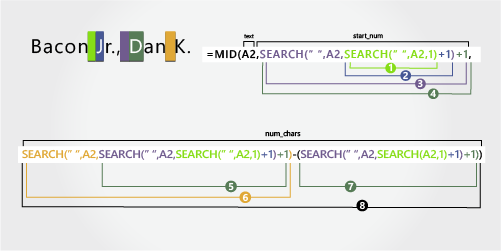
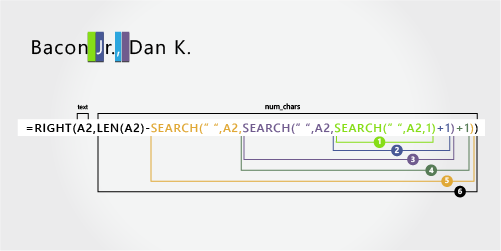
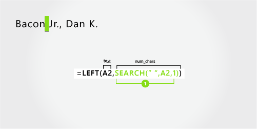
In this example, the first name is at the beginning of the string and the suffix is at the end, so you can use formulas similar to Example 2: Use the LEFT function to extract the first name, the MID function to extract the last name, and the RIGHT function to extract the suffix.

Hint Before you paste the data into the worksheet, set the column widths of columns A and B to 250.

Example name	Description
Gary Altman III	First and last name with suffix
Formula	Result (first name)
‘=LEFT(A2, SEARCH(» «,A2,1))	=LEFT(A2, SEARCH(» «,A2,1))
Formula	Result (last name)
‘=MID(A2,SEARCH(» «,A2,1)+1,SEARCH(» «,A2,SEARCH(» «,A2,1)+1)-(SEARCH(» «,A2,1)+1))	=MID(A2,SEARCH(» «,A2,1)+1,SEARCH(» «,A2,SEARCH(» «,A2,1)+1)-(SEARCH(» «,A2,1)+1))
Formula	Result (suffix)
‘=RIGHT(A2,LEN(A2)-SEARCH(» «,A2,SEARCH(» «,A2,1)+1))	=RIGHT(A2,LEN(A2)-SEARCH(» «,A2,SEARCH(» «,A2,1)+1))

First name

The first name starts at the first character from the left (G) and ends at the fifth character (the first space). Therefore, the formula extracts five characters from the left of the full name.

Search for the numeric position of the first space in A2, starting from the left. (5)
Last name

The last name starts at the sixth character from the left (A) and ends at the eleventh character (the second space). This formula involves nesting SEARCH to find the positions of the spaces.

The formula extracts six characters from the middle, starting from the sixth character.

Use the SEARCH function to find the value for start_num:

Search for the numeric position of the first space in A2, starting from the left. (5)
Add 1 to get the position of the character after the first space (A). The result is the starting position of the last name. (5 + 1 = 6)

Use nested SEARCH functions to find the value for num_chars:

Search for the numeric position of the first space in A2, starting from the left. (5)
Add 1 to get the position of the character after the first space (A). The result is the character number at which you want to start searching for the second space. (5 + 1 = 6)
Search for the numeric position of the second space in A2, starting from the sixth character found in step 4. This character number is the ending position of the last name. (12)
Search for the numeric position of the first space. (5)
Add 1 to find the numeric position of the character after the first space (A), also found in steps 3 and 4. (6)
Take the character number of the second space, found in step 5, and then subtract the character number of “A”, found in steps 6 and 7. The result is the number of characters MID extracts from the text string, starting at the sixth position, found in step 2. (12 — 6 = 6)
Suffix

The suffix starts three characters from the right. This formula involves nesting SEARCH to find the positions of the spaces.

Use nested SEARCH and the LEN functions to find the value for num_chars:

Search for the numeric position of the first space in A2, starting from the left. (5)
Add 1 to get the character after the first space (A). The result is the character number at which you want to start searching for the second space. (5 + 1 = 6)
Search for the second space in A2, starting from the sixth position (A), found in step 2. (12)
Count the total length of the text string in A2, and then subtract the number of characters from the left up to the second space, found in step 3. The result is the number of characters to be extracted from the right of the full name. (15 — 12 = 3)

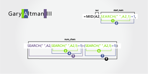
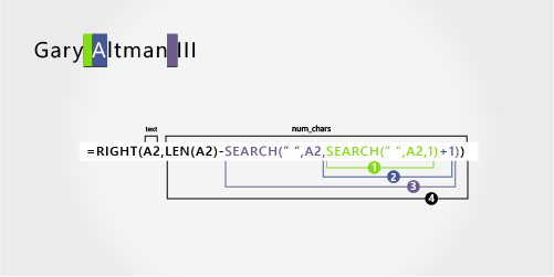
In this example, the full name is preceded by a prefix, and you use formulas similar to Example 2: the MID function to extract the first name, the RIGHT function to extract the last name.

Hint Before you paste the data into the worksheet, set the column widths of columns A and B to 250.

Example name	Description
Mr. Ryan Ihrig	With prefix
Formula	Result (first name)
‘=MID(A2,SEARCH(» «,A2,1)+1,SEARCH(» «,A2,SEARCH(» «,A2,1)+1)-(SEARCH(» «,A2,1)+1))	=MID(A2,SEARCH(» «,A2,1)+1,SEARCH(» «,A2,SEARCH(» «,A2,1)+1)-(SEARCH(» «,A2,1)+1))
Formula	Result (last name)
‘=RIGHT(A2,LEN(A2)-SEARCH(» «,A2,SEARCH(» «,A2,1)+1))	=RIGHT(A2,LEN(A2)-SEARCH(» «,A2,SEARCH(» «,A2,1)+1))

First name

The first name starts at the fifth character from the left (R) and ends at the ninth character (the second space). The formula nests SEARCH to find the positions of the spaces. It extracts four characters, starting from the fifth position.

Use the SEARCH function to find the value for the start_num:

Search for the numeric position of the first space in A2, starting from the left. (4)
Add 1 to get the position of the character after the first space (R). The result is the starting position of the first name. (4 + 1 = 5)

Use nested SEARCH function to find the value for num_chars:

Search for the numeric position of the first space in A2, starting from the left. (4)
Add 1 to get the position of the character after the first space (R). The result is the character number at which you want to start searching for the second space. (4 + 1 = 5)
Search for the numeric position of the second space in A2, starting from the fifth character, found in steps 3 and 4. This character number is the ending position of the first name. (9)
Search for the first space. (4)
Add 1 to find the numeric position of the character after the first space (R), also found in steps 3 and 4. (5)
Take the character number of the second space, found in step 5, and then subtract the character number of “R”, found in steps 6 and 7. The result is the number of characters MID extracts from the text string, starting at the fifth position found in step 2. (9 — 5 = 4)
Last name

The last name starts five characters from the right. This formula involves nesting SEARCH to find the positions of the spaces.

Use nested SEARCH and the LEN functions to find the value for num_chars:

Search for the numeric position of the first space in A2, starting from the left. (4)
Add 1 to get the position of the character after the first space (R). The result is the character number at which you want to start searching for the second space. (4 + 1 = 5)
Search for the second space in A2, starting from the fifth position (R), found in step 2. (9)
Count the total length of the text string in A2, and then subtract the number of characters from the left up to the second space, found in step 3. The result is the number of characters to be extracted from the right of the full name. (14 — 9 = 5)

This example uses a hyphenated last name. A space separates each name component.

Hint Before you paste the data into the worksheet, set the column widths of columns A and B to 250.

Example name	Description
Julie Taft-Rider	Hyphenated last name
Formula	Result (first name)
‘=LEFT(A2, SEARCH(» «,A2,1))	=LEFT(A2, SEARCH(» «,A2,1))
Formula	Result (last name)
‘=RIGHT(A2,LEN(A2)-SEARCH(» «,A2,1))	=RIGHT(A2,LEN(A2)-SEARCH(» «,A2,1))

First name

The first name starts at the first character from the left and ends at the sixth position (the first space). The formula extracts six characters from the left.

Use the SEARCH function to find the value of num_chars:

Search for the numeric position of the first space in A2, starting from the left. (6)
Last name

The entire last name starts ten characters from the right (T) and ends at the first character from the right (r).

Use the LEN and SEARCH functions to find the value for num_chars:

Search for the numeric position of the space in A2, starting from the first character from the left. (6)
Count the total length of the text string to be extracted, and then subtract the number of characters from the left up to the first space, found in step 1. (16 — 6 = 10)

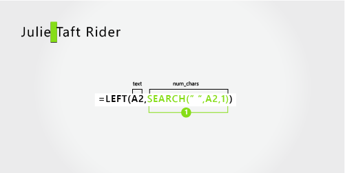
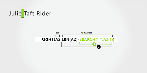
Need more help?

Источник

Working with Excel often involves rearranging the data in the worksheets.

And one common task many Excel users have to do is to cut the cell values from one cell and paste it to some other cell in the same worksheet or in another worksheet/workbook.

While this is a basic operation that most Excel users are often aware of, in case you’re a beginner, I’ll show you everything you need to know about how to cut a cell value in Excel.

Keyboard Shortcut to Cut Cell Value (or Range of Cells)

Let’s first start with the simplest and the most common way of cutting a cell value in Excel – a keyboard shortcut.

Control + X

Below are the steps to use the above keyboard shortcut to cut cell values in Excel:

Select the cell or range of cells that you want to cut
Hold the Control key on your keyboard (use the Command key instead of the Control key if you’re using a Mac)
Press the X key. You will see dancing ants (a dashed outline) around the selection

Select say where you want to copy the cell/range that you cut
Use the keyboard shortcut Control + V to paste the cut cells (hold the Control key and then press the V key)

Also read: 200+ Excel Keyboard Shortcuts – 10x Your Productivity

Cut Cells Using Mouse Drag and Drop

If you perform using your mouse over using the keyboard shortcuts, you can easily do that as well.

Below I have a dataset where I want to cut to the cells in column A and paste these in column C.

Below are the steps to do this using mouse drag and drop:

Select the range of cells that you want to cut
Place the cursor at the edge of the selection. You will notice that the cursor changes and shows a four-arrow icon (as shown below)

Cursor changes when you select the data and place the cursor at the edge

Press the left mouse key and hold it
Drag the cursor to the position where you want these cells to be pasted
Leave the mouse key

The above steps would cut the selected cells and then paste them where you have the cursor.

While you may think that these are a lot of steps compared to a keyboard shortcut, in my experience, this method is equally fast if you want to cut and paste cells in a nearby area.

Where this fails is when you want to cut the cells and paste them in some other worksheet or some other workbooks (as this only works in the same worksheet).

Also read: Boost Your Productivity with Excel Mouse Double Click Tricks

Cut Partial Cell Value Using Keyboard Shortcut

Sometimes, you may want to cut only a part of the content in a cell and not the entire cell itself.

In such a scenario, the only way to do this is to get into the edit mode in the cell, manually select the content that you want to cut, use the keyboard shortcut to cut that content, and then paste it wherever you want.

Below I have the text “It’s a Wonderful Day” in cell A1, And I want to only cut the text “Wonderful Day”.

Here are the steps to do this:

Select the cells that have the content that you want to cut (cell A1 in our example)
Double-click on the cell or press the F2 key to get into the edit mode (you’ll see the cursor blinking in the cell when you are in the edit mode)
Use your mouse to drag the cursor and select the cell that you want to cut

Use the keyboard shortcut Control + X to cut the text
Select the cell where you want to paste this text
Paste the copied content by using the keyboard shortcut Control V

While it’s possible for you to copy multiple cells and cut and paste them at the same time, when you want to cut partial text from a cell, you need to do it one cell at a time.

Note: You can also select the partial text by selecting the cell and then copying the text from the Formula Bar

In this tutorial, I showed you a simple keyboard shortcut that you can use to quickly cut and paste cell values in Excel.

I also covered how you can use the mouse drag-and-drop technique to do the same thing without using a keyboard shortcut. And I also covered how you can cut partial text from a cell in excel.

I hope you found this Excel tutorial useful.

Other Excel tutorials you may also like:

Save As Shortcuts in Excel (Quick and Easy)
Copy and Paste Multiple Cells in Excel (Adjacent & Non-Adjacent)
How to Copy and Paste Columns in Excel? 3 Easy Ways!
How to Copy and Paste Formulas in Excel without Changing Cell References
Working with Cells and Ranges in Excel VBA (Select, Copy, Move, Edit)
How to Start a New Line in Excel Cell (Keyboard Shortcut + Formula)

Источник