
Create or delete a custom list for sorting and filling data
Excel for Microsoft 365 Excel 2021 Excel 2019 Excel 2016 Excel 2013 Excel 2010 Excel 2007 More…Less
Use a custom list to sort or fill in a user-defined order. Excel provides day-of-the-week and month-of-the year built-in lists, but you can also create your own custom list.
To understand custom lists, it is helpful to see how they work and how they are stored on a computer.
Comparing built-in and custom lists
Excel provides the following built-in, day-of-the-week, and month-of-the year custom lists.
|
Built-in lists |
|
Sun, Mon, Tue, Wed, Thu, Fri, Sat |
|
Sunday, Monday, Tuesday, Wednesday, Thursday, Friday, Saturday |
|
Jan, Feb, Mar, Apr, May, Jun, Jul, Aug, Sep, Oct, Nov, Dec |
|
January, February, March, April, May, June, July, August, September, October, November, December |
Note: You cannot edit or delete a built-in list.
You can also create your own custom list, and use them to sort or fill. For example, if you want to sort or fill by the following lists, you’ll need to create a custom list, since there is no natural order.
|
Custom lists |
|
High, Medium, Low |
|
Large, Medium, and Small |
|
North, South, East, and West |
|
Senior Sales Manager, Regional Sales Manager, Department Sales Manager, and Sales Representative |
A custom list can correspond to a cell range, or you can enter the list in the Custom Lists dialog box.
Note: A custom list can only contain text or text that is mixed with numbers. For a custom list that contains numbers only, such as 0 through 100, you must first create a list of numbers that is formatted as text.
There are two ways to create a custom list. If your custom list is short, you can enter the values directly in the popup window. If your custom list is long, you can import it from a range of cells.
Enter values directly
Follow these steps to create a custom list by entering values:
-
For Excel 2010 and later, click File > Options > Advanced > General > Edit Custom Lists.
-
For Excel 2007, click the Microsoft Office Button
 > Excel Options > Popular >Top options for working with Excel > Edit Custom Lists.
 -
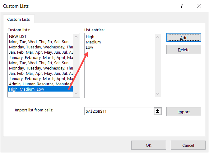
In the Custom Lists box, click NEW LIST, and then type the entries in the List entries box, beginning with the first entry.
Press the Enter key after each entry.
-
When the list is complete, click Add.
The items in the list that you have chosen will appear in the Custom lists panel.
-
Click OK twice.
 > Excel Options > Popular >Top options for working with Excel > Edit Custom Lists.
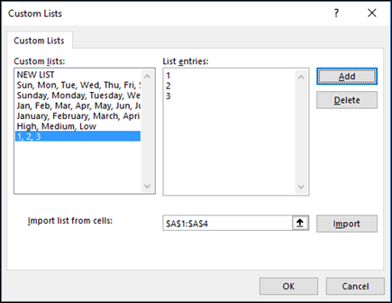
Create a custom list from a cell range
Follow these steps:
-
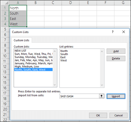
In a range of cells, enter the values that you want to sort or fill by, in the order that you want them, from top to bottom. Select the range of cells you just entered, and follow the previous instructions for displaying the Edit Custom Lists popup window.
-
In the Custom Lists popup window, verify that the cell reference of the list of items that you have chosen appears in the Import list from cells field, and then click Import.
-
The items in the list that you have chosen will appear in the Custom Lists panel.
-
Click OK twice.
Note: You can only create a custom list according to values, such as text, numbers, dates or times. You cannot create a custom list for formats such as cell color, font color, or an icon.
Follow these steps:
-
Follow the previous instructions for displaying the Edit Custom Lists dialog.
-
In the Custom Lists box, choose the list that you want to delete, and then click Delete.
Once you create a custom list, it is added to your computer registry, so that it is available for use in other workbooks. If you use a custom list when sorting data, it is also saved with the workbook, so that it can be used on other computers, including servers where your workbook might be published to Excel Services and you want to rely on the custom list for a sort.
However, if you open the workbook on another computer or server, you do not see the custom list that is stored in the workbook file in the Custom Lists popup window that is available from Excel Options, only from the Order column of the Sort dialog box. The custom list that is stored in the workbook file is also not immediately available for the Fill command.
If you prefer, add the custom list that is stored in the workbook file to the registry of the other computer or server and make it available from the Custom Lists popup window in Excel Options. From the Sort popup window, in the Order column, select Custom Lists to display the Custom Lists popup window, then select the custom list, and then click Add.
Need more help?
You can always ask an expert in the Excel Tech Community or get support in the Answers community.
Need more help?
Want more options?
Explore subscription benefits, browse training courses, learn how to secure your device, and more.
Communities help you ask and answer questions, give feedback, and hear from experts with rich knowledge.
When we need to collect data from others, they may write different things from their perspective. Still, we need to make all the related stories under one. Also, it is common that while entering the data, they make mistakes because of typo errors. For example, assume in certain cells, if we ask users to enter either “YES” or “NO,” one will enter “Y,” someone will insert “YES” like this, and we may end up getting a different kind of results. So in such cases, creating a list of values as pre-determined values allows the users only to choose from the list instead of users entering their values. Therefore, in this article, we will show you how to create a list of values in Excel.
Table of contents
- Create List in Excel
- #1 – Create a Drop-Down List in Excel
- #2 – Create List of Values from Cells
- #3 – Create List through Named Manager
- Things to Remember
- Recommended Articles
You can download this Create List Excel Template here – Create List Excel Template
#1 – Create a Drop-Down List in Excel
We can create a drop-down list in Excel using the “Data Validation in excelThe data validation in excel helps control the kind of input entered by a user in the worksheet.read more” tool, so as the word itself says, data will be validated even before the user decides to enter. So, all the values that need to be entered are pre-validated by creating a drop-down list in Excel. For example, assume we need to allow the user to choose only “Agree” and “Not Agree,” so we will create a list of values in the drop-down list.
- In the Excel worksheet under the “Data” tab, we have an option called “Data Validation” from this again, choose “Data Validation.”

- As a result, this will open the “Data Validation” tool window.
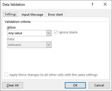
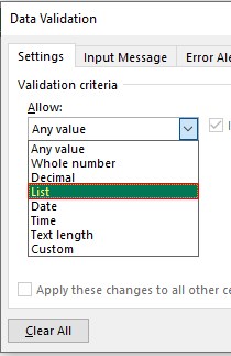
- The “Settings” tab will be shown by default, and now we need to create validation criteria. Since we are creating a list of values, choose “List” as the option from the “Allow” drop-down list.
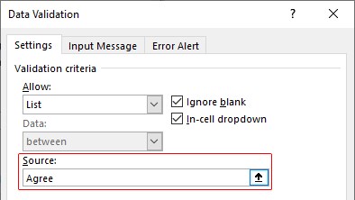
- For this “List,” we can give a list of values to be validated in the following way, i.e., by directly entering the values in the “Source” list.

- Enter the first value as “Agree.”
- Once the first value to be validated is entered, we need to enter “comma” (,) as the list separator before entering the next value. So, enter “comma” and enter the following values as “Not Agree.”
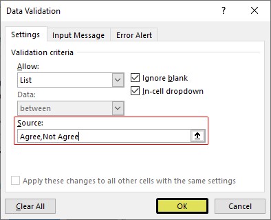
- After that, click on “Ok,” and the list of values may appear in the form of the “drop-down” list.

#2 – Create a List of Values from Cells
The above method is to get started, but imagine the scenario of creating a long list of values or your list of values changing now and then. Then, it may get difficult to return and edit the list of values manually. So, by entering values in the cell, we can easily create a list of values in Excel.
Follow the steps to create a list from cell values.
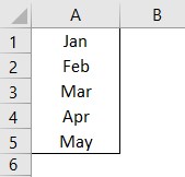
- We must first insert all the values in the cells.

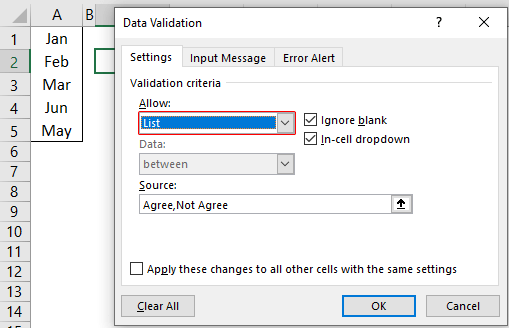
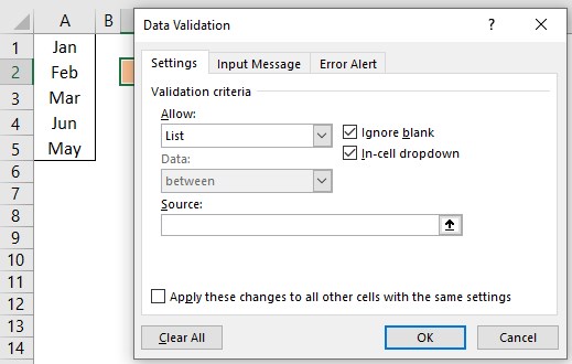
- Then, open “Data Validation” and choose the validation type as “List.”

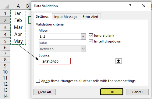
- Next, in the “Source” box, we need to place the cursor and select the list of values from the range of cells A1 to A5.

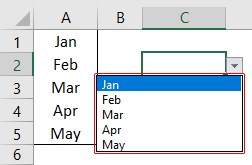
- Click on “OK,” and we will have the list ready in cell C2.

So values to this list are supplied from the range of cells A1 to A5. Any changes in these referenced cells will also impact the drop-down list.
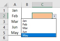
For example, in cell A4, we have a value as “Apr,” but now we will change that to “Jun” and see what happens in the drop-down list.
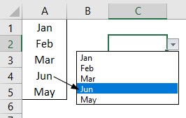
Now, look at the result of the drop-down list. Instead of “Apr,” we see “Jun” because we had given the list source as cell range, not manual entries.
#3 – Create List through Named Manager
There is another way to create a list of values, i.e., through named ranges in excelName range in Excel is a name given to a range for the future reference. To name a range, first select the range of data and then insert a table to the range, then put a name to the range from the name box on the left-hand side of the window.read more.
- We have values from A1 to A5 in the above example, naming this range “Months.”

- Now, select the cell where we need to create a list and open the drop-down list.
- Now place the cursor in the “Source” box and press the F3 key to an open list of named ranges.
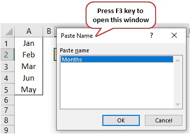
- As we can see above, we have a list of names, choose the name “Months” and click on “OK” to get the name to the “Source” box.
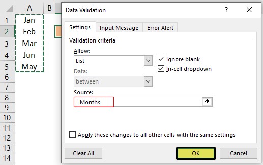
- Click on “OK,” and the drop-down list is ready.
Things to Remember
- The shortcut key to open data validation is “ALT + A + V + V.“
- We must always create a list of values in the cells so that it may impact the drop-down list if any change happens in the referenced cells.
Recommended Articles
This article has been a guide to Excel Create List. Here, we learn how to create a list of values in Excel also, create a simple drop-down method and make a list through name manager along with examples and downloadable Excel templates. You may learn more about Excel from the following articles: –
- Custom List in Excel
- Drop Down List in Excel
- Compare Two Lists in Excel
- How to Randomize List in Excel?
Create a drop-down list
- Select the cells that you want to contain the lists.
- On the ribbon, click DATA > Data Validation.
- In the dialog, set Allow to List.
- Click in Source, type the text or numbers (separated by commas, for a comma-delimited list) that you want in your drop-down list, and click OK.
Contents
- 1 How do I create a list from data in Excel?
- 2 How do I make a list column in Excel?
- 3 Can you make lists in Excel?
- 4 How do I create multiple lists in Excel?
- 5 How do I create a list of names in Excel?
- 6 How do I create a list in spreadsheet?
- 7 How do I create a custom AutoFill list in Excel 2019?
- 8 How do I create a custom list for importing the range?
- 9 How do I create a list by criteria in Excel?
- 10 How do I create a numbered list in one cell in Excel?
- 11 How do I create a dynamic Data Validation list?
- 12 How do I create a multi column Data Validation list in Excel?
- 13 How do I create a list name?
- 14 How do I create an AutoFill list?
- 15 How do I make boxes in Excel?
- 16 How do I create a list box in Excel cell?
How do I create a list from data in Excel?
Create a list based on a spreadsheet
- From the Lists app in Microsoft 365, select +New list or from your site’s home page, select + New > List.
- On the Create a list page, select From Excel.
- Choose Upload file to select a file on your device, or Choose a file already on this site.
- Enter the name for your list.
How do I make a list column in Excel?
Follow these steps:
- Select the columns to sort.
- In the ribbon, click Data > Sort.
- In the Sort popup window, in the Sort by drop-down, choose the column on which you need to sort.
- From the Order drop-down, select Custom List.
- In the Custom Lists box, select the list that you want, and then click OK to sort the worksheet.
Can you make lists in Excel?
STEP 1: Go to the File Tab. STEP 2: Select Options from the left panel. STEP 3: In the Excel Options dialog box, select Advanced. STEP 4: Under the General section, click on the Edit Custom List button.
How do I create multiple lists in Excel?
Here are the steps to create a drop-down list in Excel:
- Select the cell or range of cells where you want the drop-down list to appear (C2 in this example).
- Go to Data –> Data Tools –> Data Validation.
- In the Data Validation dialogue box, within the settings tab, select ‘List’ as Validation Criteria.
How do I create a list of names in Excel?
How to get a list of all names in the workbook
- Select the topmost cell of the range where you want the names to appear.
- Go to the Formulas tab > Define Names group, click Use in Formulas, and then click Paste Names… Or, simply press the F3 key.
- In the Paste Names dialog box, click Paste List.
How do I create a list in spreadsheet?
Create a drop-down list
- Open a spreadsheet in Google Sheets.
- Select the cell or cells where you want to create a drop-down list.
- Click Data.
- Next to “Criteria,” choose an option:
- The cells will have a Down arrow.
- If you enter data in a cell that doesn’t match an item on the list, you’ll see a warning.
- Click Save.
How do I create a custom AutoFill list in Excel 2019?
Create your own AutoFill Series
Click the File tab. Click the Excel Options button to open the Excel Options dialog box. Click the Advanced button [A] and scroll to the bottom of the Advanced Options window. Click the Edit Custom Lists button [B] to open the Custom Lists dialog box.
How do I create a custom list for importing the range?
To create a custom list from existing items that you’ve listed in a worksheet range, click in the Import list from cells box, select the range on the sheet, and then click Import.
How do I create a list by criteria in Excel?
In Excel, sometimes you may need to generate a list based on criteria.
Generate List Based on Criteria
- Using INDEX-SMALL Combination.
- Using the AGGREGATE Function.
- Unique List Using INDEX-MATCH-COUNTIF.
- Using FILTER Function.
How do I create a numbered list in one cell in Excel?
Fill a column with a series of numbers
- Select the first cell in the range that you want to fill.
- Type the starting value for the series.
- Type a value in the next cell to establish a pattern.
- Select the cells that contain the starting values.
- Drag the fill handle.
How do I create a dynamic Data Validation list?
Creating a Dynamic Drop Down List in Excel (Using OFFSET)
- Select a cell where you want to create the drop down list (cell C2 in this example).
- Go to Data –> Data Tools –> Data Validation.
- In the Data Validation dialogue box, within the Settings tab, select List as the Validation criteria.
How do I create a multi column Data Validation list in Excel?
Excel 2007 and above
- Data tab / Data Validation module.
- In the name text box : name the range as List.
- Create a list of validations in E3 (Data/Validation, in Allow: select “List” in Source: type =List)
- Open the Name manager: Formula tab/set name/Name Manager, select the name of the range (List)
How do I create a list name?
To name cells, or ranges, based on worksheet labels:
- Select the labels and the cells that are to be named.
- On the Ribbon, click the Formulas tab, then click Create from Selection.
- In the Create Names From Selection window, add a check mark for the location of the labels, then click OK.
- Click on a cell to see its name.
How do I create an AutoFill list?
Select File→Options→Advanced (Alt+FTA) and then scroll down and click the Edit Custom Lists button located in the General section. The Custom Lists dialog box opens with its Custom Lists tab, where you now should check the accuracy of the cell range listed in the Import List from Cells text box.
How do I make boxes in Excel?
How to Make Boxes in Excel
- Open your spreadsheet.
- Click Insert.
- Select the Text Box button.
- Draw the text box in the desired spot.
How do I create a list box in Excel cell?
Add a list box to a worksheet
- Create a list of items that you want to displayed in your list box like in this picture.
- Click Developer > Insert.
- Under Form Controls, click List box (Form Control).
- Click the cell where you want to create the list box.
- Click Properties > Control and set the required properties:
![]()
Download Article
![]()
Download Article
If you’re wondering how to create a multiple-line list in a single cell in Microsoft Excel, you’ve come to the right place. Whether you want a cell to contain a bulleted list with line breaks, a numbered list, or a drop-down list, inserting a list is easy once you know where to look. This wikiHow will teach you three helpful ways to insert any type of list to one cell in Excel.
-
1
Double-click the cell you want to edit. If you want to create a bullet or numerical list in a single cell with each item on its own line, start by double-clicking the cell into which you want to type the list.
-
2
Insert a bullet point (optional). If you want to preface each list item with a bullet rather than a number or other character, you can use a key shortcut to insert the bullet symbol. Here’s how:
- Mac: Press Option + 8.
-
Windows:
- If you have a numeric keypad on the side of your keyboard, hold down the Alt key while pressing 7 on the keypad.[1]
- If not, click the Insert menu, select Symbol, type 2022 into the «Character code» box at the bottom, and then click Insert.
- If 2022 didn’t bring up a bullet point, select the Wingdings font instead, and then enter 159 as the character code. You can then click Insert to add the bullet point.
- If you have a numeric keypad on the side of your keyboard, hold down the Alt key while pressing 7 on the keypad.[1]
Advertisement
-
3
Type your first list item. Don’t press Enter or Return after typing.
- If you want your list to be numbered, preface the first list item with 1. or 1).
-
4
Press Alt+↵ Enter (PC) or Control+⌥ Option+⏎ Return on a Mac. This adds a line break so you can start typing on the next line of the same cell.[2]
-
5
Type the remaining list items. To continue your list, just enter another bullet point on the second line, type the list item, and press Alt + Enter or Control + Option + Return to open a new line. When you’re finished, you can click anywhere else on your sheet to exit the cell.


Advertisement
-
1
Create your list in another app. If you’re trying to paste a bullet list (or other type of list) into a single cell rather than have it spread across multiple cells, there’s a trick to pasting the list. Start by creating your list in an app like Word, TextEdit, or Notepad.
- If you create a bulleted list in Word, the bullets will copy over to your cell when pasted into Excel. Bullets may not copy from other apps.
-
2
Copy the list. To do this, just highlight the list, right-click the highlighted area, and then select Copy.
-
3
Double-click a cell in Excel. Double-clicking the cell before pasting makes it so the list items will all appear in the same cell.
-
4
Right-click the cell. The context menu will expand.
-
5
Click the clipboard icon under «Paste Options.» The icon has a clipboard and a black rectangle. This pastes the list into the cell you double-clicked. Each list item will appear on its own line within the same cell.


Advertisement
-
1
Open the workbook in which you want to create a drop-down list. If you want to be able to click a cell to view and select from a drop-down list, you can create a list with Excel’s data validation tool.[3]
-
2
Create a new worksheet in the workbook. You can do this by clicking the + next to the existing workbook sheets at the bottom of Excel. This worksheet is where you’ll enter the items that you want to appear in your drop-down list.
- After you create the list on a separate sheet and add it to a table, you’ll be able to create a drop-down list containing the list data in any cell you want.
-
3
Type each list item into a single column. Enter every possible list choice into its own separate cell. The items you type will all be available in the drop-down list.
- If you plan to make a lot of drop-down menus and want to use this same sheet to create all of them, add a header to the top of the list. For example, if you’re making a list of cities, you could type City into the first cell. This header won’t actually appear on the drop-down list you create—it’s just for organization on this sheet that contains list data.
-
4
Highlight the entire table and press Ctrl+T. Include the header at the top of the list when highlighting. This opens the Create Table dialog.
-
5
Choose a header option and click OK. If you added a header to the top of your list, check the box next to «My table has headers.» If not, make sure there is no checkmark there before clicking OK.
- Now that your list is in a table, you can make changes to it after creating your drop-down list, and your drop-down list will update automatically.
-
6
Sort the list alphabetically. This will keep your list organized once you add it to your sheet. To do this, just click the arrow next to your header cell and select Sort A to Z.
-
7
Click the cell on the worksheet in which you want to add the list. This can be any cell on any worksheet in the workbook.
-
8
Type a name for the list into the cell. This is the cell where the list will appear, so give it a name that indicates the type of option you should choose from that list. For example, if you made a list of cities, you could type City here.
-
9
Click the Data tab and select Data Validation. Make sure the cell is selected before doing this. If you don’t see Data Validation in the toolbar, click the icon in the «Data Tools» section that has two black rectangles with a green checkmark and a red circle with a line through it. This opens the Data Validation window.
-
10
Click the «Allow» menu and select List. Additional options will expand.
-
11
Click the up-arrow in the «Source» field. This minimizes the Data Validation window so you can select your list data.
-
12
Select the list (without the header) and press ↵ Enter or ⏎ Return. Click back over to the tab that has your list data and drag the mouse cursor over just the list items. Pressing Enter or Return will add the range to the «Source» field.
-
13
Click OK. The selected cell now has a drop-down list. If you need to add or remove items from the list, you can simply make those changes on your new worksheet and they’ll automatically propagate to the list.


Advertisement
Ask a Question
200 characters left
Include your email address to get a message when this question is answered.
Submit
Advertisement
Thanks for submitting a tip for review!
About This Article
Article SummaryX
1. Double-click the cell.
2. Press Alt + 7 or Option + 8 to add a bullet point.
3. Type a list item.
4. Press Alt + Enter (PC) or Control + Option + Return (Mac) to go to the next line.
5. Repeat until your list is finished.
Did this summary help you?
Thanks to all authors for creating a page that has been read 62,222 times.
Is this article up to date?
A Custom List in Excel is very handy to fill a range of cells with your own personal list.
It could be a list of your team members at work, countries, regions, phone numbers, or customers. The main goal of a custom list is to remove repetitive work and manual errors.
It is extremely useful when you need to fill in the same data from time to time. There are two options to create a list in Excel that can be used repeatedly by using the fill handle.
In this tutorial, you will learn how to create a list in Excel:
- Using Pre-existing List
- Create a list in Excel manually
- Import from another worksheet
Let’s look at each of these methods one-by-one!
Watch it on YouTube and give it a thumbs-up!

Download this Excel Workbook and follow along with the tutorial on how to create a list in Excel :
Using Pre-existing List
At first, it might seem like magic how Excel does this!
There are some lists that are already stored in Excel like days of the week and months in a year.

To demonstrate the power of Excel’s Custom Lists, we’ll explore what’s currently in Excel’s memory as a default list:
STEP 1: Type February in the first cell

STEP 2: From that first cell, click the lower right corner and drag it to the next 5 cells to the right

STEP 3: Release and you will see it get auto-populated to July (The succeeding months after February)

Create a list in Excel manually
You can also manually add new values in the Custom List box and re-use them whenever you wish to.
Let us go straight into the Options in Excel to view how it’s being done, and how you can create your own Custom List:
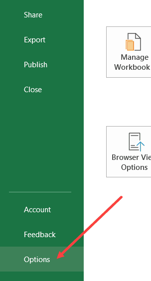
STEP 1: Select the File tab

STEP 2: Click Options

STEP 3: Select the Advanced option

STEP 4: Scroll all the way down and under the General section, click Edit Custom Lists.

Here you can see the built-in default Excel lists of the calendar months and the days.
If you click on a Custom List, you will see under List entries that it is greyed out and you cannot make any changes. This indicated that it is a default Excel Custom List.

STEP 5: You can create & add your own Custom List under the List entries section.
Click on NEW LIST under the Custom Lists area and then manually enter your list, entering one entry per line:

After typing the values, click Add.
In our screenshot below, we added the values of the Greek alphabet (alpha, beta, gamma, and so on)
Click OK once done.

STEP 6: Click OK again

STEP 7: Now let’s go back into our Excel workbook to see our new Custom List in action. Type alpha on a cell.

STEP 8: From that cell, click the lower right corner and drag it to the next 5 cells to the right

STEP 9: Release and you will see it get auto-populated to zeta, which is based on our Custom List created in Step 8

Next up is a demonstration of how to make a list in Excel by importing data from another worksheet.
Import from another worksheet
You can easily import a custom list from another worksheet. Follow the steps below to get this done:
STEP 1: Go to the File Tab.

STEP 2: Select Options from the left panel.

STEP 3: In the Excel Options dialog box, select Advanced.

STEP 4: Under the General section, click on the Edit Custom List button.

STEP 5: In the Custom List dialog box, select the small arrow up button.

STEP 6: Select the range containing the custom list.

STEP 7: Click on Import.

STEP 8: Once the list will appear under list entries and click OK.

STEP 9: Click OK.

Now, your custom list is stored in Excel!
STEP 10: Type the first entry of the list “XS” in cell A8.

STEP 11: From that first cell, click the lower right corner and drag it to the next 6 cells to the right.

The entire list will be displayed in the selected range!

You can even create this list vertically. Simply, type the XS in a cell. Click on the lower right corner and drag the cell downwards.

The list will appear vertically!
Conclusion
In this article, you have learned how to make a list in Excel so that you don’t have to type the same list over and over again. You use the Custom list feature in Excel and store it in Excel and use it whenever necessary.
You can either use the pre-existing list, manually type the list or link it from another worksheet!
Make sure to download our FREE PDF on the 333 Excel keyboard Shortcuts here:

You can learn more about how to use Excel by viewing our FREE Excel webinar training on Formulas, Pivot Tables, Power Query, and Macros & VBA!

Excel has some useful features that allow you to save time and be a lot more productive in your day-to-day work.
One such useful (and less-known) feature in the Custom Lists in Excel.
Now, before I get to how to create and use custom lists, let me first explain what’s so great about it.
Suppose you have to enter numbers the month names from Jan to Dec in a column. How would you do it? And no, doing it manually is not an option.
One of the fastest ways would be to have January in a cell, February in an adjacent cell and then use the fill handle to drag and let Excel automatically fill in the rest. Excel is smart enough to realize that you want to fill the next month in each cell in which you drag the fill handle.
Month names are quite generic and therefore it’s available by default in Excel.
But what if you have a list of department names (or employee names or product names), and you want to do the same. Instead of manually entering these or copy-paste these, you want these to appear magically when you use the fill handle (just like month names).
You can do that too…
… by using Custom Lists in Excel
In this tutorial, I will show you how to create your own custom lists in Excel and how to use these to save time.
How to Create Custom Lists in Excel
By default, Excel already has some pre-fed custom lists that you can use to save time.
For example, if you enter ‘Mon’ in one cell ‘Tue’ in an adjacent cell, you can use the fill handle to fill the rest of the days. In case you extend the selection, keep on dragging and it will repeat and give you the day’s name again.

Below are the custom lists that are already in-built in Excel. As you can see, these are mostly days and month names as these are fixed and will not change.

Now, suppose you want to create a list of departments that you often need in Excel, you can create a custom list for it. This way, the next time you need to get all the departments name in one place, you don’t need to rummage through old files. All you need to do is type the first two in the list and drag.

Below are the steps to create your own Custom List in Excel:
- Click the File tab

- Click on Options. This will open the ‘Excel Options‘ dialog box

- Click on the Advanced option in the left-pane

- In the General option, click on the ‘Edit Custom Lists’ button (you may have to scroll down to get to this option)

- In the Custom Lists dialog box, import the list by selecting the range of cells that have the list. Alternatively, you can also enter the name manually in the List Entries box (separated by comma or each name in a new line)

- Click on Add


As soon as you click on Add, you would notice that your list now becomes a part of the Custom Lists.

In case you have a large list that you want to add to Excel, you can also use the Import option in the dialog box.
Pro tip: You can also create a named range and use that named range to create the custom list. To do this, enter the name of the named range in the ‘Import list from cells’ field and click OK. The benefit of this is that you can change or expand the named range and it will automatically get adjusted as the custom list
Now that you have the list in Excel backend, you can use it just like you use numbers or month names with Autofill (as shown below).

While it’s great to be able to quickly get these custom lits names in Excel by doing a simple drag and drop, there is something even more awesome that you can do with custom lists (that’s what the next section is about).
Create Your Own Sorting Criteria Using Custom Lists
One great thing about custom lists is that you can use it to create your own sorting criteria. For example, suppose you have a dataset as shown below and you want to sort this based on High, Medium, and Low.

You can’t do this!
If you sort alphabetically, it would screw the alphabetical order (it will give you High, Low, and Medium and not High, Medium, and Low).
This is where Custom Lists really shine.
You can create your own list of items and then use these to sort the data. This way, you will get all the High values together at the top followed by the medium and low values.
The first step is to create a custom list (High, Medium, Low) using the steps shown in the previous section (‘How to Create Custom Lists in Excel‘).
Once you have the custom list created, you can use the below steps to sort based on it:
- Select the entire dataset (including the headers)
- Click the Data tab

- In the Sort and Filter group, click on the Sort icon. This will open the Sort dialog box

- In the Sort dialog box, make the following selections:
- Sort by Column: Priority
- Sort On: Cell Values
- Order: Custom Lists. When the dialog box opens, select the sorting criteria you want to use and then click on OK.

- Click OK


The above steps would instantly sort the data using the list you created and used as criteria while sorting (High, Medium, Low in this example).

Note that you don’t necessarily need to create the custom list first to use it in sorting. You can use the above steps and in Step 4 when the dialog box opens, you can create a list right there in that dialog box.
Some Examples Where you can Use Custom Lists
Below are some of the cases where creating and using custom lists can save you time:
- If you have a list that you need to enter manually (or copy-paste from some other source), you can create a custom list and use that instead. For example, this could be department names in your organization, or product names or regions/countries.
- If you’re a teacher, you can create a list of your student names. That way, when you are grading them the next time, you don’t need to worry about entering the student names manually or copy-pasting it from some other sheet. This also ensures that there are fewer chances of errors.
- When you need to sort data based on criteria that are not in-built in Excel. As covered in the previous section, you can use your own sorting criteria by making a custom list in Excel.
So this is all that you need to know about Creating Custom Lists in Excel.
I hope you found this useful.
You may also like the following Excel tutorials:
- How to Sort by the Last Name in Excel
- How to SORT in Excel (by Rows, Columns, Colors, Dates, & Numbers)
- How to Sort By Color in Excel
- How to Sort Worksheets in Excel
- Automatically Sort Data in Alphabetical Order using Formula
Bottom Line: Learn 4 different techniques for creating a list of numbers in Excel. These include both static and dynamic lists that change when items are added or deleted from the list.
Skill Level: Beginner
Watch the Tutorial
Download the Excel File
You can download the worksheet that I use in the video here:
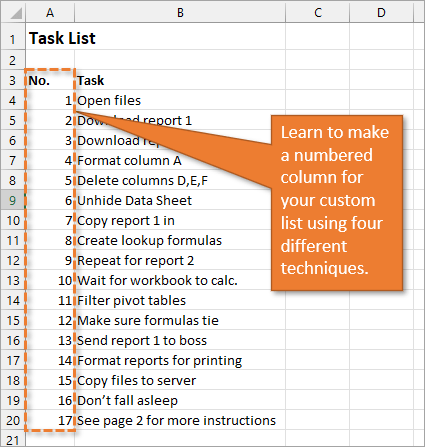
If you have a list of items in Excel and you’d like to insert a column that numbers the items, there are several ways to accomplish this. Let’s look at four of those ways.
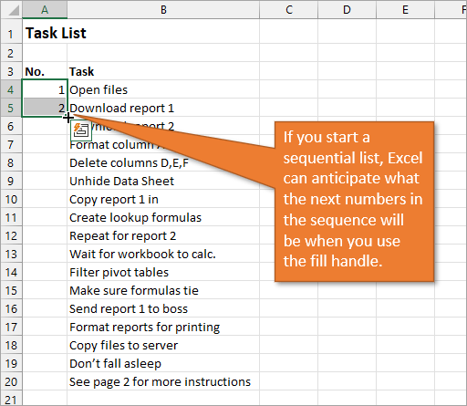
1. Create a Static List Using Auto-Fill
The first way to number a list is really easy. Start by filling in the first two numbers of your list, select those two numbers, and then hover over the bottom right corner of your selection until your cursor turns into a plus symbol. This is the fill handle.
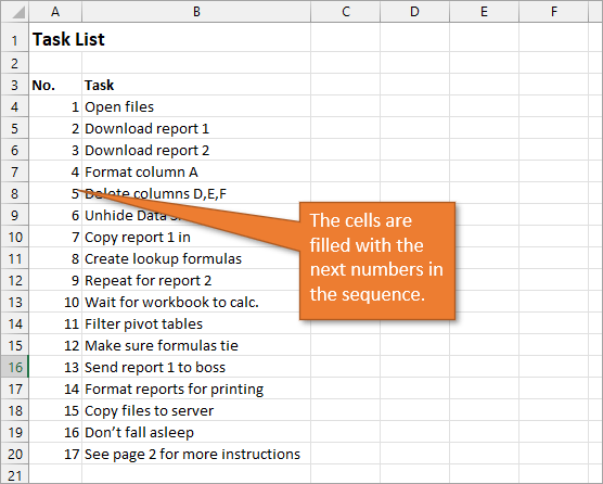
When you double-click on that fill handle (or drag it down to the end of your list), Excel will fill in the blanks with the next numbers in the sequence.
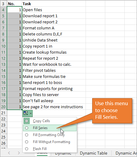
An alternate way to create this same numbered list is to type a 1 in the first cell and then double-click the fill handle. Because Excel doesn’t have a second number to identify a sequence or pattern, it will fill down the columns with 1s. But you will notice that a menu is available at the end of your column, and from that menu, you can select the option to Fill Series. This will change the 1s to a sequential list of numbers.
The numbered column we’ve created in both instances is static. This means it doesn’t change when you make additions or deletions to the corresponding list of items. For example, if I insert a new row in order to add another task, there is a break in the numbered column as well, and I would have to repeat the same steps to correct the list.
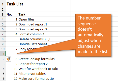
So, unless we want the numbers to always remain as they are, a better option would be to create a dynamic list.
2. Create a Dynamic List Using a Formula
We can use formulas to create a dynamic list where the numbers update when we add or delete rows from the list.
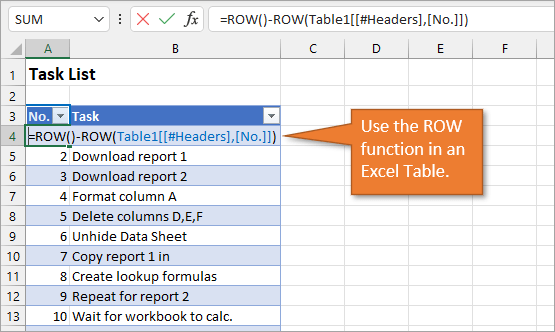
To use a formula for creating a dynamic number list, we can use the ROW function. The ROW function returns the row number of a cell. If we don’t specify a cell for ROW, it just returns the current row number of whatever is selected.
In our example, the first cell in our list doesn’t start on Row 1. It starts on Row 4. But we don’t want our list to start at 4; we want it to start at 1. To subtract the extra 3, our formula will include a minus sign and then the ROW function again, but this time pointed to the cell above our formula (which is in Row 3).
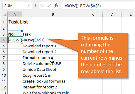
We use the absolute values (dollar signs) in our cell selection because we don’t want that number to change as we copy the formula down the list. In other words, we always want to subtract 3 from the row number to give us our list number.
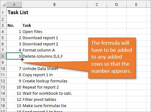
When we copy down the formula, we have a numbered list that will adjust when we add or delete rows. However, when adding a row, we will have to copy the formula into the newly inserted cell.
This additional step of copying the formula into new rows can be avoided if we use Excel Tables.
3. Create a Dynamic List Using a Formula in an Excel Table
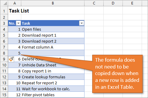
If we write the same formula but we use an Excel table, the only difference we will make in the formula is that we reference the column header instead of the absolute cell value.
Because we are using an Excel Table, the formula automatically fills down to the other rows. When we add a row to the table, the formula will automatically populate in the new cell.
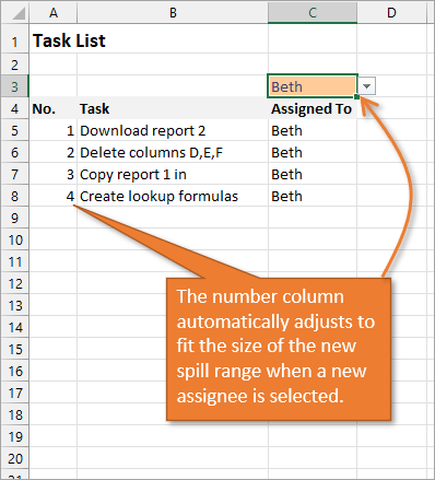
4. Create a Dynamic List Using Dynamic Array Formulas
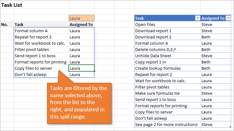
Below, I have a table that is populated using Dynamic Array Formulas. The FILTER formula spills a range of results based on whatever name is selected in the orange cell.
The Dynamic Array formula we will use is SEQUENCE. This will return a sequence for the number of rows we identify in the formula. To tell Excel how many rows there are, we will use the ROW function as the argument for sequence. The argument for ROW is just the spill range. The way to notate the spill range is to simply place a hashtag after the name of the first cell in the range. So our formula looks like this:
=SEQUENCE(ROWS(B5#))
Once we complete our formula and hit Enter, the list will be numbered.
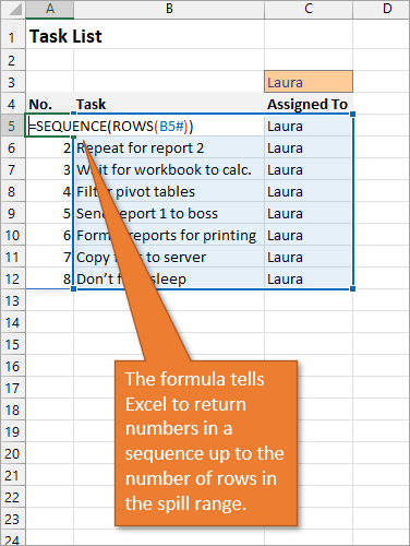
With this formula in place, if the size of the range changes when a new name is selected, the numbered column for the list will automatically adjust as well.
Bonus Tip: Formatting Your Numbered List
If you want to add periods or other punctuation to your numbered list:
- Select the entire list and right-click to choose Format Cells. Or use the keyboard shortcut Ctrl + 1.
- Choose the Custom option on the Number tab.
- Then in the Type field, type in the number 0 with whatever punctuation you would like to surround your number.
Here, I’ve just added a period.
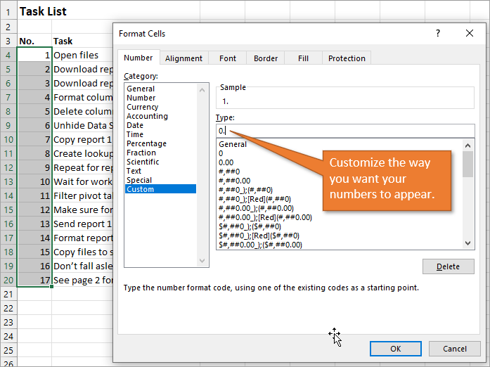
When you hit OK, you will have formatted the entire selection.
Related Posts
Here are a few similar posts that may interest you.
- Excel Tables Tutorial Video – Beginners Guide for Windows & Mac
- New Excel Features: Dynamic Array Formulas & Spill Ranges
- How to Prevent Excel from Freezing or Taking A Long Time when Deleting Rows
Conclusion
I hope these four ways to create ordered lists are helpful for you. If you have questions or feedback, I would love to hear them in the comments. Have a great week!
The human mind is a powerful thing.
But sometimes, it can suddenly blank out!
Like forgetting to note down the grocery items missing in your pantry or the project changes your client wants by the end of the day.
While our brain can do quite a lot, sometimes relying on our memory isn’t always the best way to keep track of our tasks.
That’s why a to-do list in Excel can be helpful.
It helps you break down your tasks into different sections on a single spreadsheet, which you can view at any time.
In this article, we’ll cover the six steps to create a to-do list in Excel and also discuss a better alternative that can handle more complex requirements the easier way.
Let’s roll!

What Is a To Do List in Excel?
A to-do list in Microsoft Excel helps you organize your most essential tasks in a tabular form. It comes with rows and columns to add a new task, dates, and other specific notes.
Basically, it lets you assemble all your to-dos on a single spreadsheet.
Whether you’re preparing a move-in checklist or a project task list, a to-do list in Excel can simplify your work process and store all your information.
While there are other powerful apps for creating to-do lists, people use Excel because:
- It’s a part of the Microsoft Office Suite people are familiar with
- It offers powerful conditional formatting rules and data validation for analysis and calculations
- It includes an array of reporting tools like matrices, charts, and pivot tables, making it easier to customize the data
In fact, you can create Excel to-do lists for a wide range of activities, including project management, client onboarding, travel itinerary, inventory, and event management.
Without further ado, let’s learn how to create a to-do list in Excel.
6 Simple Steps To Make a To Do List in Excel
Here’s a simple step-by-step guide on how to make a to-do list in Excel.
Step 1: Open a new Excel file
To open a new file, click on the Excel app, and you’ll find yourself at the Excel Home page. Double-click on the Blank Workbook to open a new Excel spreadsheet.

If you’re already on an Excel sheet and want to open a new file:
- Click on the File tab, which will take you to the backstage view. Here you can create, save, open, print, and share documents
- Select New, then click on Blank Workbook
Want an even faster route?
Press Ctrl+N after opening Excel to create a Blank Workbook.
Your new workbook is now ready for you.
Step 2: Add column headers
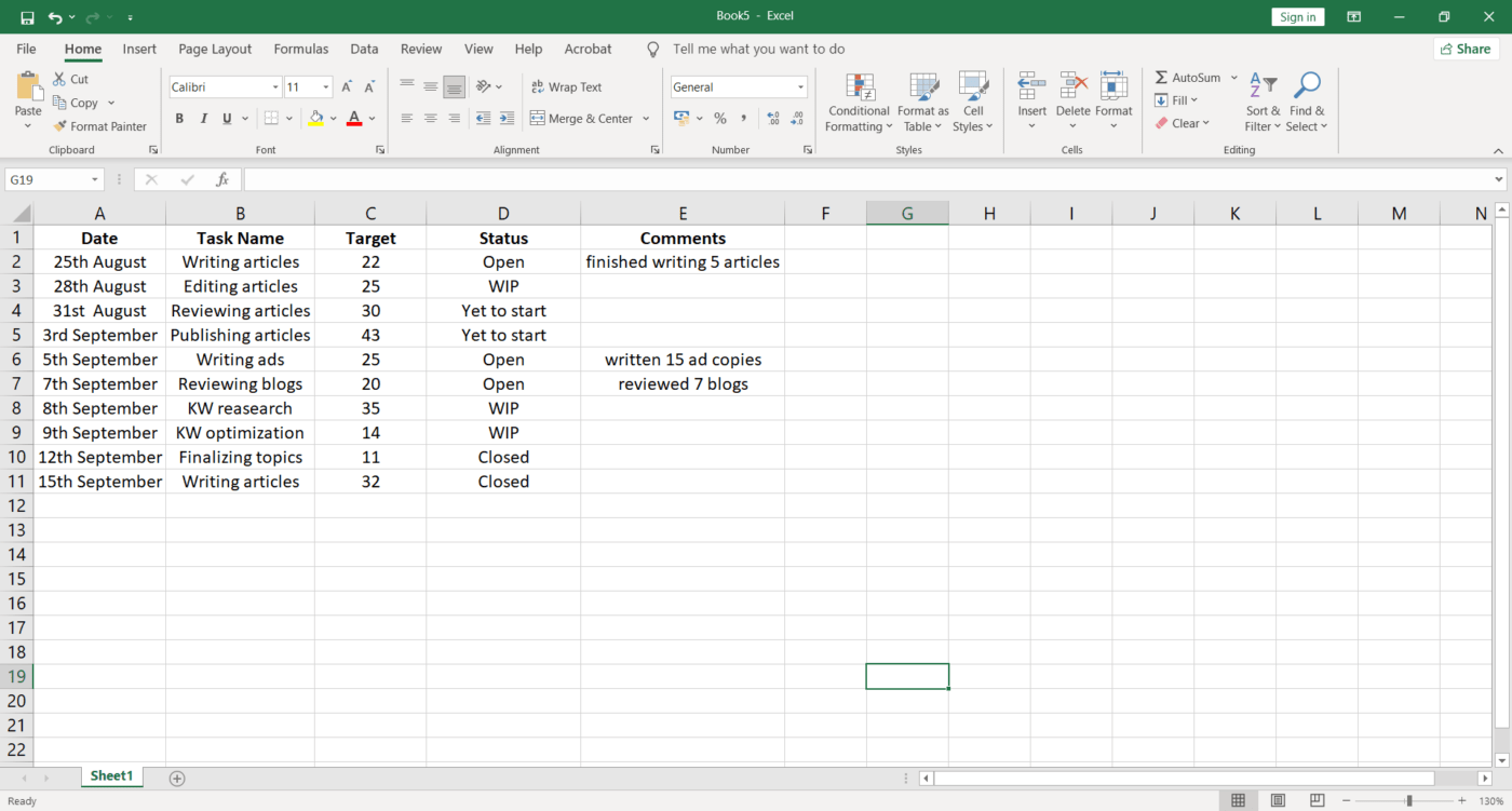
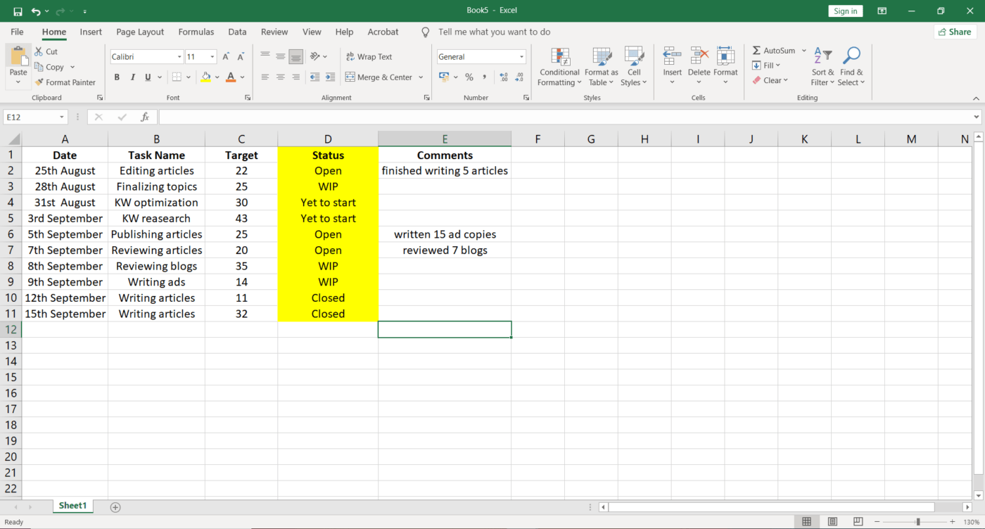
In our Excel to-do list, we want to track tasks and keep an eye on the progress by adding the column headers: Date, Task Name, Target, Status, and Comments. You can enter the column headers across the top row of the spreadsheet.
These column headers will let anyone viewing your spreadsheet get the gist of all the information under it.
Step 3: Enter the task details
Enter your task details under each column header to organize your information the way you want.
In our to-do list table, we have collated all the relevant information we want to track:
- Date: mentions the specific dates
- Task Name: contains the name of our tasks
- Target: the number of task items we aim to complete
- Status: reflects our work progress
You can also fix the alignment of your table by selecting the cells you want and click on the icon for center alignment from the Home tab.
Step 4: Apply filters
Too many to-dos?
Use the Filter option in Excel to retrieve data that matches particular criteria.
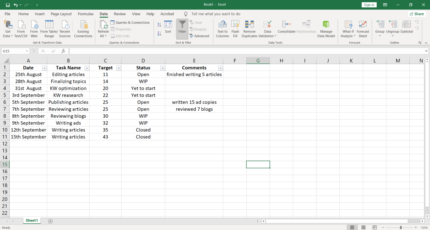
All you need to do is select any cell within the range of your data (A1-E11) > Select Data > then select Filter.
You’ll see drop-down lists appearing in the header of each column, as shown in the image below.
Click on the drop-down arrow for the column you want to apply a filter.

As shown in our to-do list table below, we want to apply the filter to the Status column, so we’ve selected the cell range of D1-D11.
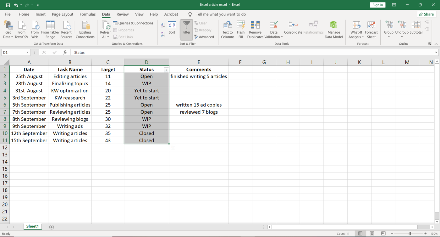
Then, in the Filter menu that appears, you can uncheck the boxes next to the data you don’t want to view and click OK. You can also quickly uncheck all by clicking on Select All.
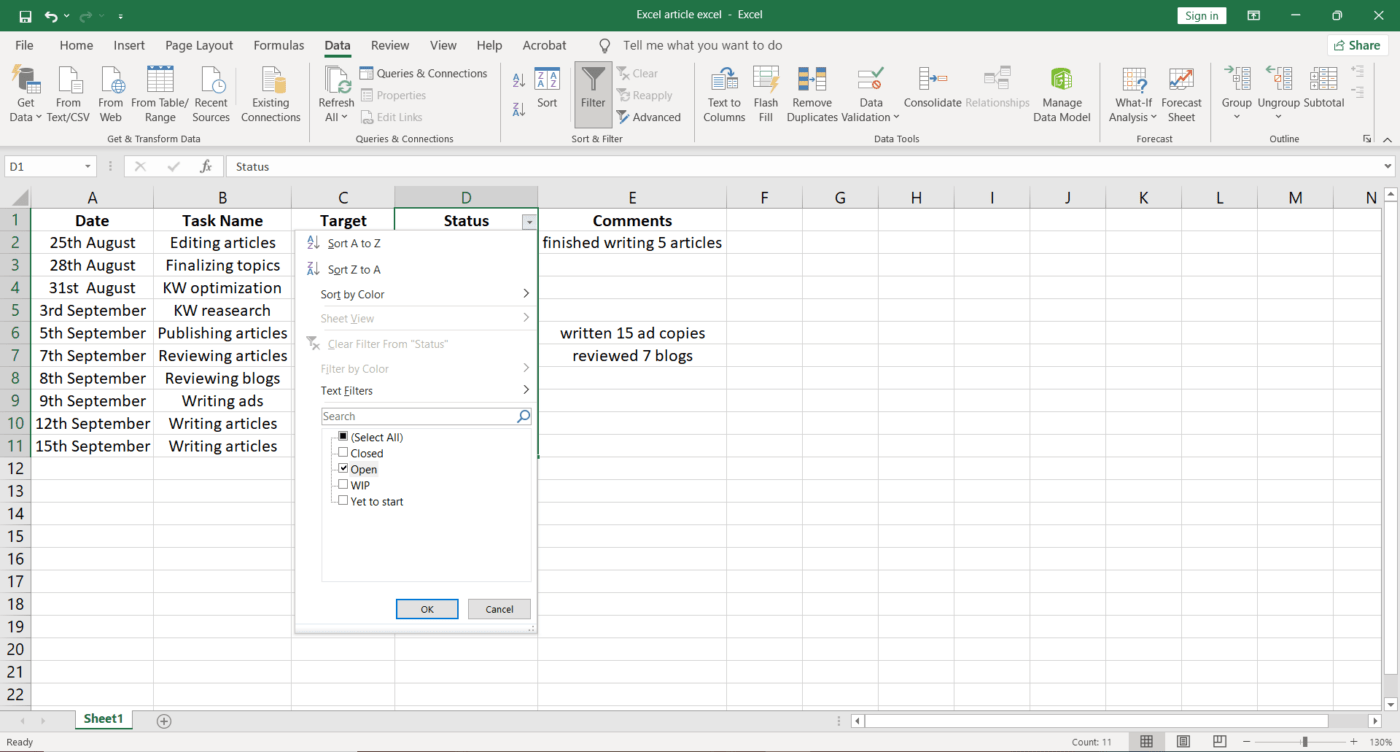
In our to-do list, we want to view only the Open tasks, so we apply the filter for that data.
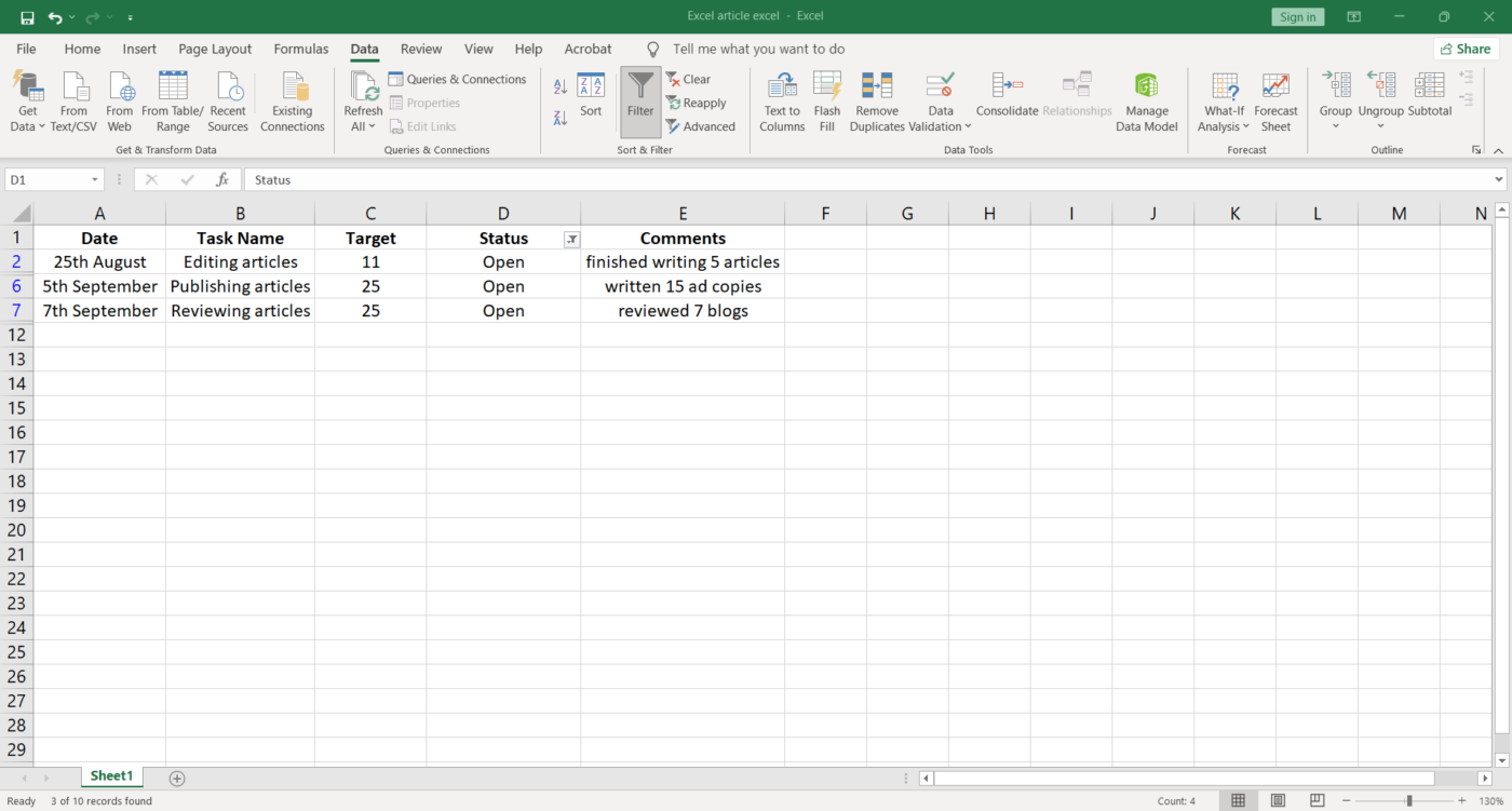
After you save this Excel file, the filter will be there automatically the next time you open the file.
Step 5: Sort the data
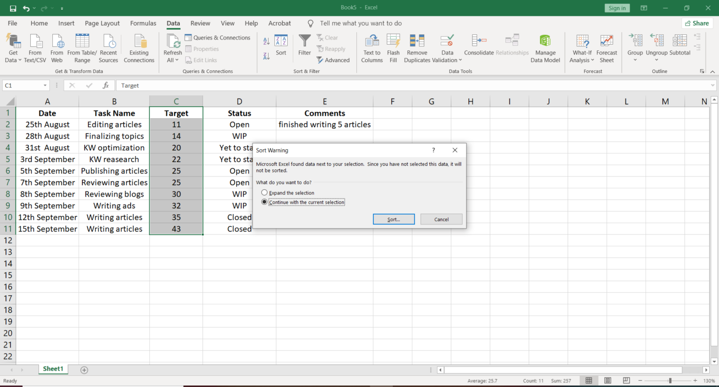
You can use the Sort option in Excel to quickly visualize and understand your data better.
We want to sort the data in the Target column, so we’ll select the cell range C1-C11. Click on the Data tab and select Sort.
A Sort Warning dialog box will appear asking if you want to Expand the selection or Continue with the current selection. You can choose the latter option and click on Sort.
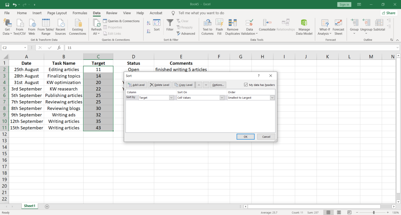
The Sort dialog box will open where you have to enter the:
- The column you want to Sort by
- Cell values you wish to Sort on
- Order in which you want to sort the data
For our table, we have chosen the Target column and kept the order from smallest to largest.
Step 6: Edit and customize your to do list
You can edit fields, add columns, use colors and fonts to customize your to-do list the way you want.
Like in our table, we’ve highlighted the Status column so anybody viewing can quickly understand your task progress.
And voila! ✨
We’ve created a simple Excel to-do list that can help you keep track of all your tasks.
Want to save more time?
Create a template from your existing workbook to keep the same formatting options that you generally use while making your to-do lists.
Or you can use any to-do list Excel template to get started instantly.
10 Excel To Do List Templates
Templates can help keep your workbooks consistent, especially when they’re related to a particular project or client. For example, a daily Excel to-do list template improves efficiency and enables you to complete your tasks sooner.
Here are a few Excel to-do list templates that can help improve efficiency and save time:
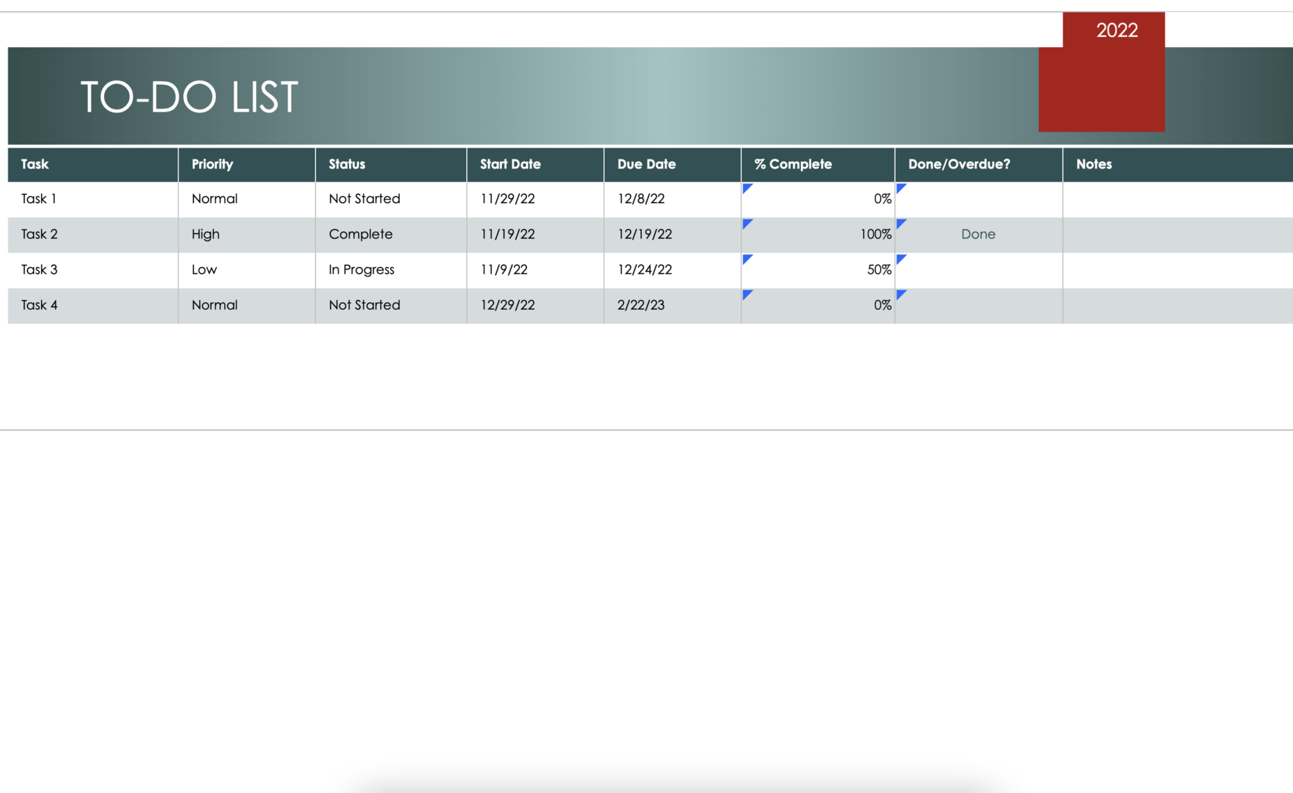
1. Excel project management task list template
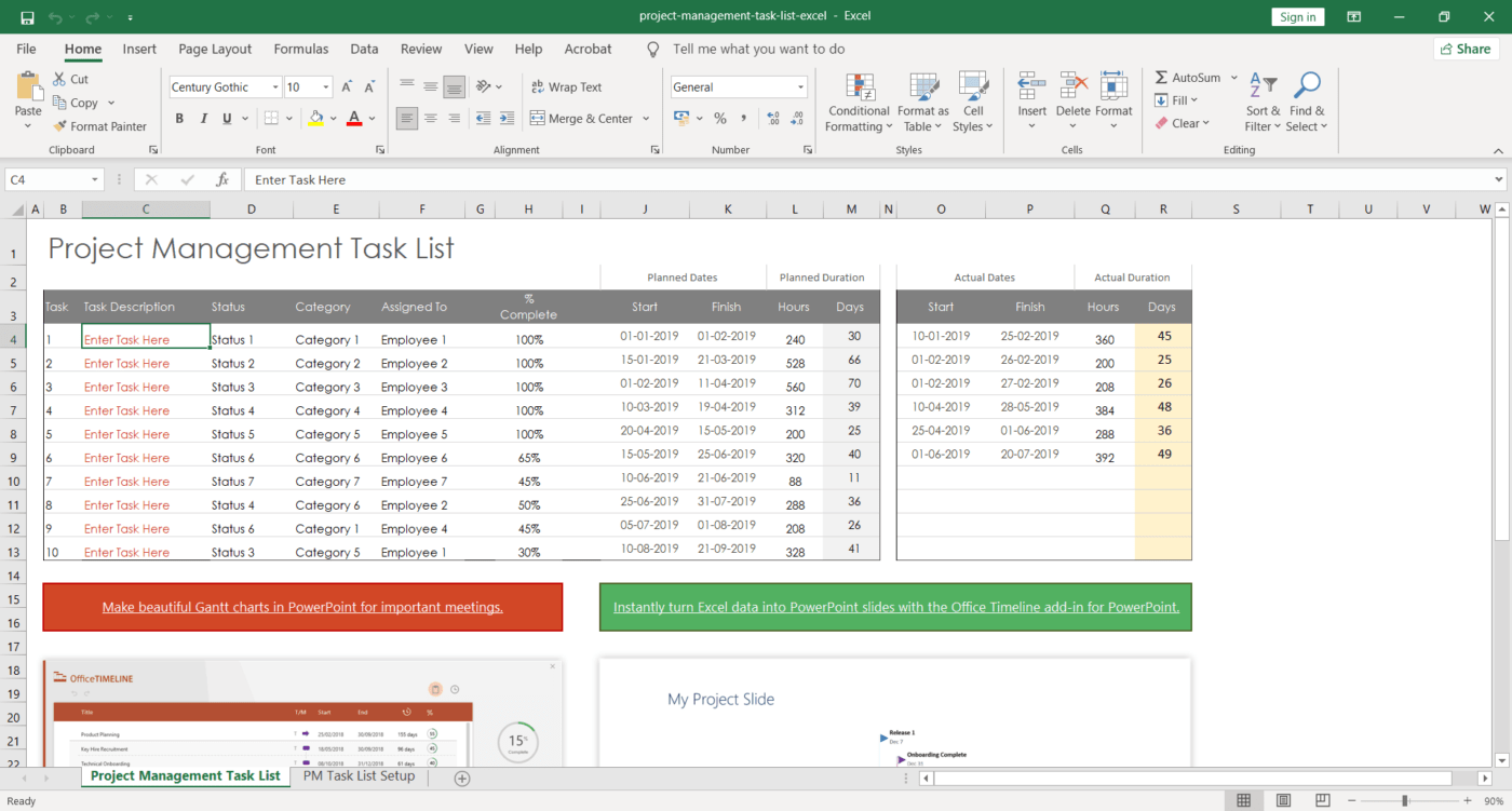
Download this project management task list template.
2. Excel inventory list template
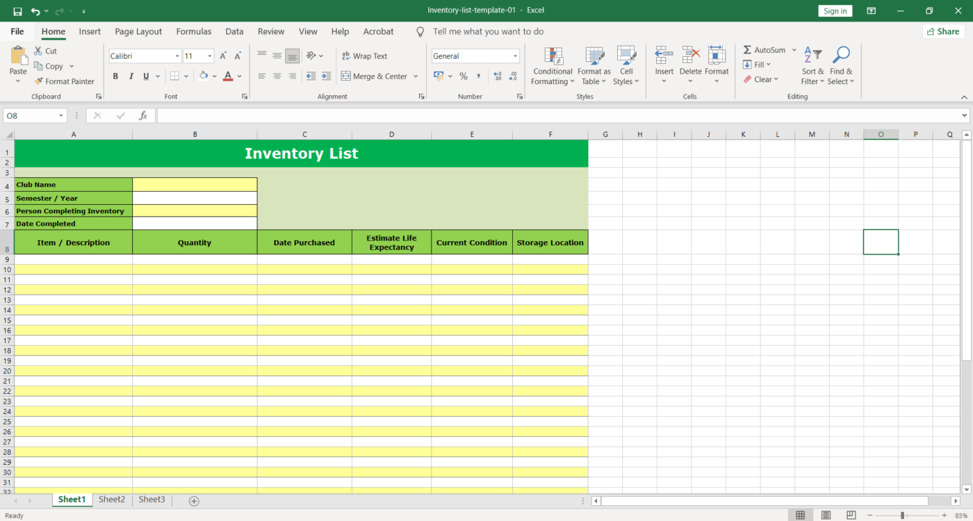
Download these inventory list templates.
3. Excel action item list template
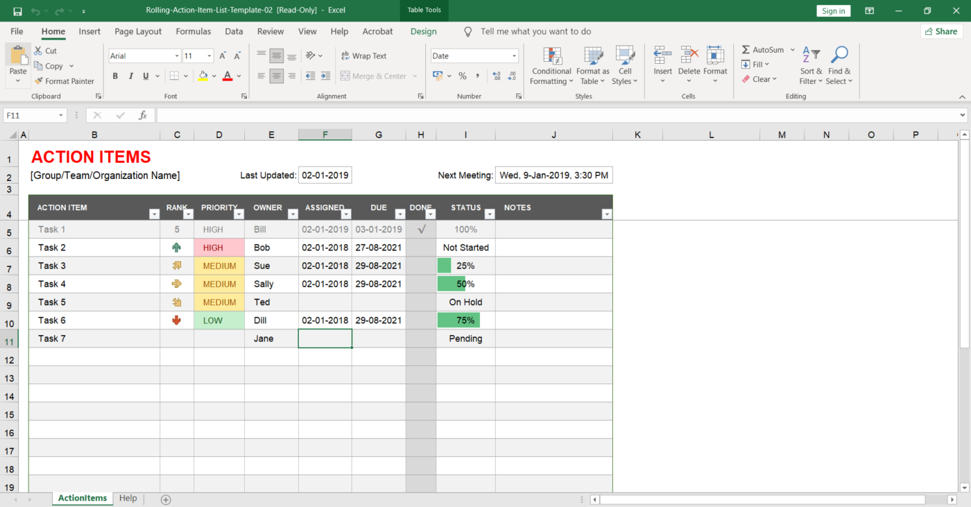
Download this action item list template.
4. Excel simple to-do list template
Download this simple to-do list template.
5. Excel bill paying checklist template
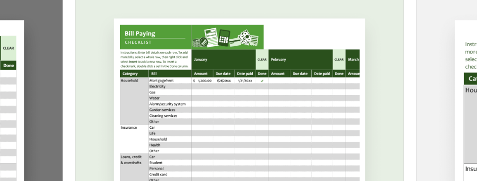
Download this bill paying checklist template.
6. Excel weekly assignment to-do list template
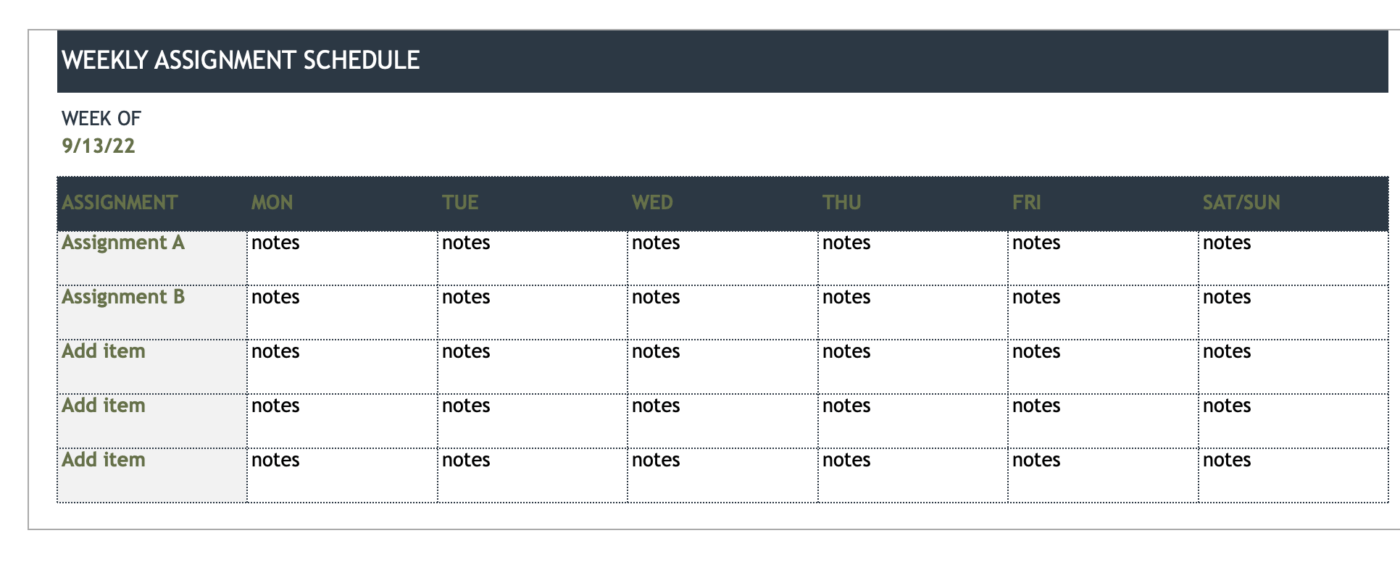
Download this weekly assignment template.
7. Excel prioritized to-do list template
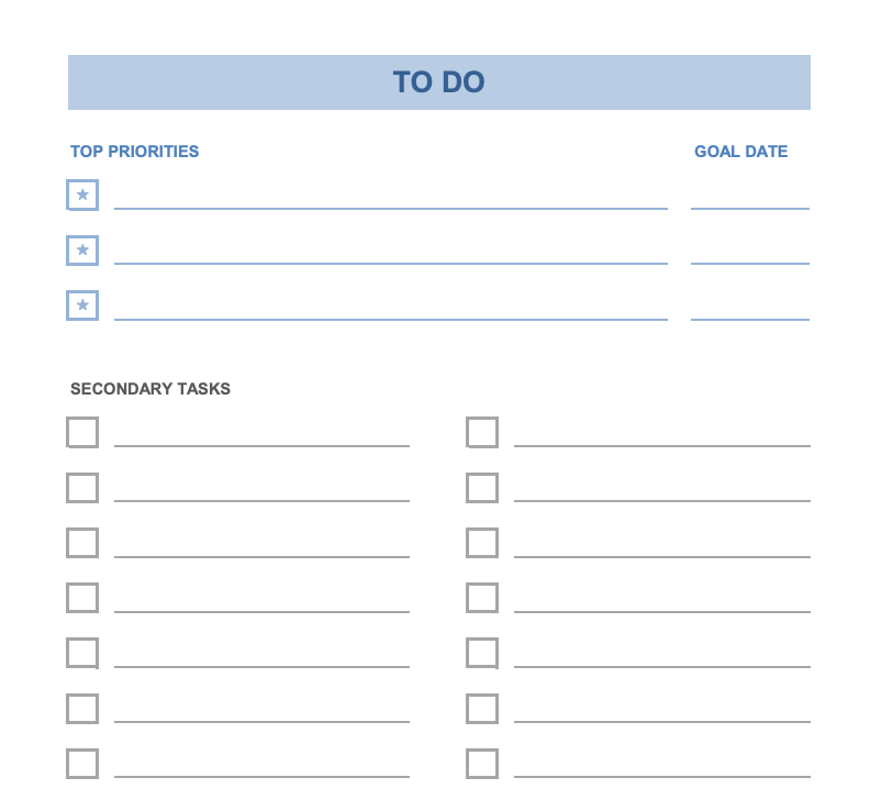
Download this prioritized to-do list template.
8. Excel homework to-do list template
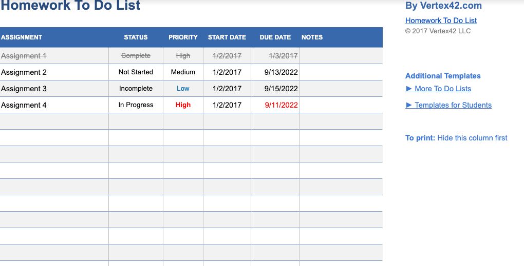
Download this homework to-do list template.
9. Excel to-do list with deadlines template
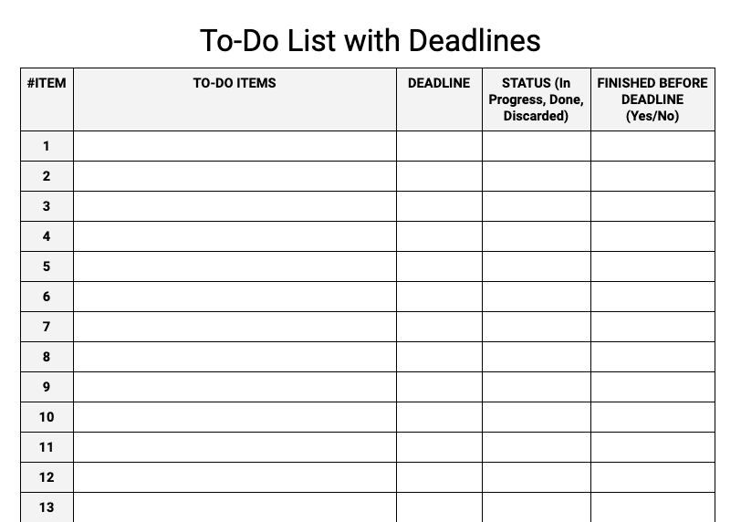
Download this to-do list with deadlines template.
10. Excel project task list template
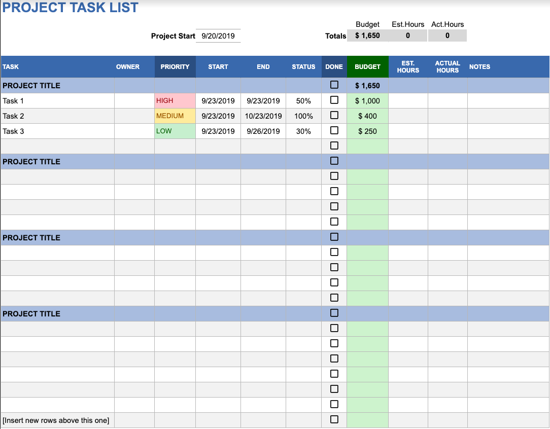
Download this project task list template.
However, you can’t always find a template that will fulfill your specific needs.
Additionally, data management in Excel is prone to human error.
Each time a user copy-pastes information from one spreadsheet to another, there is a greater risk of new errors cropping up into successive reports.
Before you commit to Excel to-do lists, here are some limitations to consider.
3 Major Disadvantages of To Do Lists in Excel
Even though widely used, Excel spreadsheets aren’t always the best option for creating your to-do lists.
Here are the three common disadvantages of using Excel for to-do lists:
1. Lack of ownership
When multiple individuals work on the same spreadsheet, you’re unable to tell who’s editing.
You might end up repeating a task in vain if a person forgets to update the Work Status column in shared to-do lists after it’s done.
Additionally, people can easily alter task details, values, and other entries in the to-do lists (intentionally or unintentionally). You won’t know whom to hold accountable for the error or change!
2. Inflexible templates
Not all of the Excel to-do templates you find online are reliable. Some of them are extremely difficult to manipulate or customize.
You’ll spend forever on the internet to find one that works for you.
3. Manual labor
Making to-do lists in Excel involves a significant amount of manual labor.
It may take you quite some time to fill out your to-do items and create an organized system.
This doesn’t sit well with us because tons of project management tools can save you so much time and effort by creating and managing your to dos.
Moreover, the complexity increases with the increasing size of data in your Excel file. Naturally, you’d want a substitute to streamline your to-dos to track them and reduce the monotonous, manual work involved.
And honestly, Excel is no to-do list app.
To manage to-dos, you need a tool that’s specifically designed for it.
Like ClickUp, one of the highest-rated productivity and project management software that lets you create and manage to-dos with ease.
Related Excel guides:
- How to create a Kanban board in Excel
- How to create a burndown chart in Excel
- How to create a flowchart in Excel
- How to make an org chart in Excel
- How to create a dashboard in Excel
Create To Do Lists Effortlessly With ClickUp
ClickUp can help you create smart to-do lists to organize your tasks.
From adding Due Dates to setting Priorities, ClickUp’s comprehensive features let you create and conquer all your to-dos!
How?
One word: Checklists!
ClickUp’s Checklists give you the perfect opportunity to organize your task information so you never miss even the smallest of details.
All you need to do is click on Add beside To Do (you can find it within any ClickUp task), then select Checklist. You can name your Checklist and start adding the action items. Easy!

Easily organize task information so you never miss a beat with Checklists in ClickUp
Checklists within ClickUp give your tasks a clear outline. Apart from noting down the essential details, you also get subtasks to break down your tasks further.
You can also arrange and rearrange the checklist items with the easy drag-and-drop feature.

Reorganize your ClickUp Checklist by dragging and dropping your items
Worried about some tasks getting overlooked?
With ClickUp, you can add Assignees to your specific to-dos to see things through.

Manage items on your Checklist by assigning them to yourself or the team in ClickUp
It also lets you reuse your favorite Checklist Templates to scale your work efficiency.
To choose a template:
- Click Add from the To Do section of any task
- Click Checklist to reveal your options
- Choose a template and select Use Template
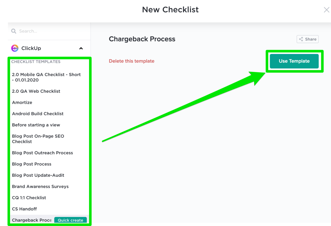
Use ClickUp’s Checklist Templates to stay efficient with different recurring tasks
Still hung up on Excel? That’s okay.
ClickUp’s Table view can help you move on.
But our Table view isn’t a mere matrix of rows and columns.
You can visualize your data clearly and create Custom Fields to record almost anything from task progress to file attachments and 15+ other field types.
Moreover, you can easily import your ongoing project details into ClickUp with our Excel and CSV import options!
But wait, that’s not all!
Here are some other ClickUp features that’ll make you forget Excel in an instant:
- Assign Task: assign tasks to one or Multiple Assignees to quicken your pace of work
- Custom Tags: effectively organize your task details by adding Tags
- Task Dependencies: help your teammates understand their to-dos concerning other tasks by setting Dependencies
- Recurring Tasks: save your time and effort by streamlining repetitive to-dos
- Google Calendar Sync: easily sync your Google Calendar events with the ClickUp Calendar view. Any updates in your Google Calendar will automatically reflect on ClickUp too
- Smart Search: search Docs easily and other items that you’ve recently created, updated, or closed
- Custom Statuses: denote the status of your tasks, so the team knows at which stage of the workflow they currently are
- Notepad: jot down ideas quickly with our portable, digital Notepad
- Embed view: declutter your screen and add the apps or websites alongside your tasks instead
- Gantt Charts: track work progress, assignees, and dependencies with a simple drag and drop functionality (check out this Excel dependencies guide)
Tame Your To Do Lists With ClickUp
Excel may be a decent option for planning daily to-dos and simple task lists. However, when you work with multiple teammates and tasks, Excel might not be ideal for what you need. Collaboration isn’t easy, there’s too much manual labor, and no team accountability.
That’s why you need a robust to-do list tool to help you manage tasks, track deadlines, follow work progress, and foster team collaboration.
Fortunately, ClickUp brings all of this to the table and so much more.
You can create to-dos, set Reminders, track Goals, and view insightful Reports.
Switch to ClickUp for free and quit wasting all that brainpower on simple to-do lists!
It’s easy to keep track of specific information
Updated on March 11, 2021
What to Know
- Select a cell > Home tab > Sort & Filter > Filter. Next, select a column header arrow to filter or sort the data.
- To guard against data errors, leave no blank rows or columns in the table.
An Excel spreadsheet can hold an enormous amount of data; Excel has built-in tools to help you find specific information when you want to retrieve it. Here’s how to create, filter, and sort a data list in Excel 2019, 2016, 2013, 2010; Excel for Microsoft 365; Excel Online; and Excel for Mac.
Create a Data List in Excel
After you’ve correctly entered data into a table and included the proper headers, convert the table to a list.
-
Select a cell in the table.
-
Select Home > Sort & Filter > Filter.
-
Column header arrows appear to the right of each header.
-
When you select a column header arrow, a filter menu appears. This menu contains options to sort the list by any of the field names and to search the list for records that match certain criteria.
-
Sort your data list to find whatever specific data you want to retrieve.
Note that a table of data must contain at least two data records before a list is created.
Basic Excel Table Information
The basic format for storing data in Excel is a table. In a table, data is entered in rows. Each row is known as a record. Once a table has been created, use Excel’s data tools to search, sort, and filter the records to find specific information.
Columns
While rows in the table are referred to as records, the columns are known as fields. Each column needs a heading to identify the data it contains. These headings are called field names. Field names are used to ensure that the data for each record is entered in the same sequence.
Make sure to enter the data in a column using a consistent format. For example, If numbers are entered as digits (such as 10 or 20,) keep it up; don’t change partway through and begin entering numbers as words (such as «ten» or «twenty»).
It’s also important to leave no blank columns in the table, and note that the table must contain at least two columns before a list is created.
Guard Against Data Errors
When creating the table, make sure the data is entered correctly. Data errors caused by incorrect data entry are the source of many problems related to data management. If the data is entered correctly in the beginning, you’ll get the results you want.
To guard against data errors, leave no blank rows in the table being created, not even between the headings and the first row of data. Make sure each record contains data about only one specific item, and that each record contains all the data about that item. There can’t be information about an item in more than one row.
Thanks for letting us know!
Get the Latest Tech News Delivered Every Day
Subscribe