
Format a date the way you want
Excel for Microsoft 365 Excel for Microsoft 365 for Mac Excel for the web Excel 2021 Excel 2021 for Mac Excel 2019 Excel 2019 for Mac Excel 2016 Excel 2016 for Mac Excel 2013 Excel 2010 Excel 2007 Excel for Mac 2011 More…Less
When you enter some text into a cell such as «2/2″, Excel assumes that this is a date and formats it according to the default date setting in Control Panel. Excel might format it as «2-Feb». If you change your date setting in Control Panel, the default date format in Excel will change accordingly. If you don’t like the default date format, you can choose another date format in Excel, such as «February 2, 2012″ or «2/2/12″. You can also create your own custom format in Excel desktop.
Follow these steps:
-
Select the cells you want to format.
-
Press CTRL+1.
-
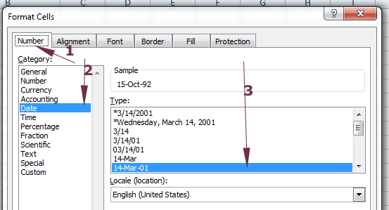
In the Format Cells box, click the Number tab.
-
In the Category list, click Date.

-
Under Type, pick a date format. Your format will preview in the Sample box with the first date in your data.
Note: Date formats that begin with an asterisk (*) will change if you change the regional date and time settings in Control Panel. Formats without an asterisk won’t change.
-
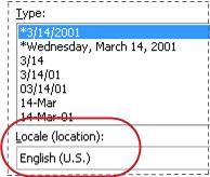
If you want to use a date format according to how another language displays dates, choose the language in Locale (location).

Tip: Do you have numbers showing up in your cells as #####? It’s likely that your cell isn’t wide enough to show the whole number. Try double-clicking the right border of the column that contains the cells with #####. This will resize the column to fit the number. You can also drag the right border of the column to make it any size you want.
If you want to use a format that isn’t in the Type box, you can create your own. The easiest way to do this is to start from a format this is close to what you want.
-
Select the cells you want to format.
-
Press CTRL+1.
-
In the Format Cells box, click the Number tab.
-
In the Category list, click Date, and then choose a date format you want in Type. You can adjust this format in the last step below.
-
Go back to the Category list, and choose Custom. Under Type, you’ll see the format code for the date format you chose in the previous step. The built-in date format can’t be changed, so don’t worry about messing it up. The changes you make will only apply to the custom format you’re creating.
-
In the Type box, make the changes you want using code from the table below.
|
To display |
Use this code |
|---|---|
|
Months as 1–12 |
m |
|
Months as 01–12 |
mm |
|
Months as Jan–Dec |
mmm |
|
Months as January–December |
mmmm |
|
Months as the first letter of the month |
mmmmm |
|
Days as 1–31 |
d |
|
Days as 01–31 |
dd |
|
Days as Sun–Sat |
ddd |
|
Days as Sunday–Saturday |
dddd |
|
Years as 00–99 |
yy |
|
Years as 1900–9999 |
yyyy |
If you’re modifying a format that includes time values, and you use «m» immediately after the «h» or «hh» code or immediately before the «ss» code, Excel displays minutes instead of the month.
-
To quickly use the default date format, click the cell with the date, and then press CTRL+SHIFT+#.
-
If a cell displays ##### after you apply date formatting to it, the cell probably isn’t wide enough to show the whole number. Try double-clicking the right border of the column that contains the cells with #####. This will resize the column to fit the number. You can also drag the right border of the column to make it any size you want.
-
To quickly enter the current date in your worksheet, select any empty cell, press CTRL+; (semicolon), and then press ENTER, if necessary.
-
To enter a date that will update to the current date each time you reopen a worksheet or recalculate a formula, type =TODAY() in an empty cell, and then press ENTER.
When you enter some text into a cell such as «2/2″, Excel assumes that this is a date and formats it according to the default date setting in Control Panel. Excel might format it as «2-Feb». If you change your date setting in Control Panel, the default date format in Excel will change accordingly. If you don’t like the default date format, you can choose another date format in Excel, such as «February 2, 2012″ or «2/2/12″. You can also create your own custom format in Excel desktop.
Follow these steps:
-
Select the cells you want to format.
-
Press Control+1 or Command+1.
-
In the Format Cells box, click the Number tab.
-
In the Category list, click Date.
-
Under Type, pick a date format. Your format will preview in the Sample box with the first date in your data.
Note: Date formats that begin with an asterisk (*) will change if you change the regional date and time settings in Control Panel. Formats without an asterisk won’t change.
-
If you want to use a date format according to how another language displays dates, choose the language in Locale (location).
Tip: Do you have numbers showing up in your cells as #####? It’s likely that your cell isn’t wide enough to show the whole number. Try double-clicking the right border of the column that contains the cells with #####. This will resize the column to fit the number. You can also drag the right border of the column to make it any size you want.
If you want to use a format that isn’t in the Type box, you can create your own. The easiest way to do this is to start from a format this is close to what you want.
-
Select the cells you want to format.
-
Press Control+1 or Command+1.
-
In the Format Cells box, click the Number tab.
-
In the Category list, click Date, and then choose a date format you want in Type. You can adjust this format in the last step below.
-
Go back to the Category list, and choose Custom. Under Type, you’ll see the format code for the date format you chose in the previous step. The built-in date format can’t be changed, so don’t worry about messing it up. The changes you make will only apply to the custom format you’re creating.
-
In the Type box, make the changes you want using code from the table below.
|
To display |
Use this code |
|---|---|
|
Months as 1–12 |
m |
|
Months as 01–12 |
mm |
|
Months as Jan–Dec |
mmm |
|
Months as January–December |
mmmm |
|
Months as the first letter of the month |
mmmmm |
|
Days as 1–31 |
d |
|
Days as 01–31 |
dd |
|
Days as Sun–Sat |
ddd |
|
Days as Sunday–Saturday |
dddd |
|
Years as 00–99 |
yy |
|
Years as 1900–9999 |
yyyy |
If you’re modifying a format that includes time values, and you use «m» immediately after the «h» or «hh» code or immediately before the «ss» code, Excel displays minutes instead of the month.
-
To quickly use the default date format, click the cell with the date, and then press CTRL+SHIFT+#.
-
If a cell displays ##### after you apply date formatting to it, the cell probably isn’t wide enough to show the whole number. Try double-clicking the right border of the column that contains the cells with #####. This will resize the column to fit the number. You can also drag the right border of the column to make it any size you want.
-
To quickly enter the current date in your worksheet, select any empty cell, press CTRL+; (semicolon), and then press ENTER, if necessary.
-
To enter a date that will update to the current date each time you reopen a worksheet or recalculate a formula, type =TODAY() in an empty cell, and then press ENTER.
When you type something like 2/2 in a cell, Excel for the web thinks you’re typing a date and shows it as 2-Feb. But you can change the date to be shorter or longer.
To see a short date like 2/2/2013, select the cell, and then click Home > Number Format > Short Date. For a longer date like Saturday, February 02, 2013, pick Long Date instead.
-
If a cell displays ##### after you apply date formatting to it, the cell probably isn’t wide enough to show the whole number. Try dragging the column that contains the cells with #####. This will resize the column to fit the number.
-
To enter a date that will update to the current date each time you reopen a worksheet or recalculate a formula, type =TODAY() in an empty cell, and then press ENTER.
Need more help?
You can always ask an expert in the Excel Tech Community or get support in the Answers community.
Need more help?
Choose from a list of date formats
- Select the cells you want to format.
- Press CTRL+1.
- In the Format Cells box, click the Number tab.
- In the Category list, click Date.
- Under Type, pick a date format.
Contents
- 1 Why can’t I change the date in Excel?
- 2 How do you change date from DD MM to yyyy in Excel?
- 3 How do I change date and time to just date in Excel?
- 4 What is the formula to change date format in Excel?
- 5 How do I extract date from datetime in Excel?
- 6 How do I extract date from text in Excel?
- 7 How do I convert 8 digits to dates in Excel?
- 8 How do I pull the Year out of a date in Excel?
- 9 How do I convert datetime to date?
- 10 How do I convert date and time to date?
- 11 How does Excel convert numbers to dates?
- 12 What is the Datevalue function in Excel?
- 13 How do I change a date in Excel to 6 digits?
- 14 How do you change the year in a date in Excel?
- 15 How do I change the year in Excel?
- 16 How do I convert a long date to a short date in Excel?
- 17 How do you change the date in a table?
Why can’t I change the date in Excel?
Try this method if Excel doesn’t change the date format
Click the Data tab from the top menu of your screen. Choose the Text to columns option from the menu. Tick the box next to the option Delimited to activate it. Press the Next button two times to move through the setup pages.
How do you change date from DD MM to yyyy in Excel?
To change the date display in Excel follow these steps:
- Go to Format Cells > Custom.
- Enter dd/mm/yyyy in the available space.
How do I change date and time to just date in Excel?
Convert date/time format cell to date only with formula
Select a blank cell you will place the date value, then enter formula =MONTH(A2) & “/” & DAY(A2) & “/” & YEAR(A2) into the formula bar and press the Enter key.
What is the formula to change date format in Excel?
Convert date to yyyy-mm-dd format with formula
1. Select a blank cell next to your date, for instance. I1, and type this formula =TEXT(G1, “yyyy-mm-dd”), and press Enter key, then drag AutoFill handle over the cells needed this formula. Now all dates are converted to texts and shown as yyyy-mm-dd format.
Extract date from a date and time
- Generic formula. =INT(date)
- To extract the date part of a date that contains time (i.e. a datetime), you can use the INT function.
- Excel handles dates and time using a scheme in which dates are serial numbers and times are fractional values.
- Extract time from a date and time.
Convert text dates by using the DATEVALUE function
- Enter =DATEVALUE(
- Click the cell that contains the text-formatted date that you want to convert.
- Enter )
- Press ENTER, and the DATEVALUE function returns the serial number of the date that is represented by the text date. What is an Excel serial number?
How do I convert 8 digits to dates in Excel?
To do this, select a cell or a range of cells with the numbers you want to convert to dates and press Ctrl + 1 to open the Format Cells dialog box. On the Number tab, choose Date, select the desired date format in Type and click OK. If have any issues I will be here to help you. Thanks!
How do I pull the Year out of a date in Excel?
To extract the year from a cell containing a date, type =YEAR(CELL) , replacing CELL with a cell reference. For instance, =YEAR(A2) will take the date value from cell A2 and extract the year from it.
How do I convert datetime to date?
MS SQL Server – How to get Date only from the datetime value?
- Use CONVERT to VARCHAR: CONVERT syntax: CONVERT ( data_type [ ( length ) ] , expression [ , style ] )
- You can also convert to date: SELECT CONVERT(date, getdate()); It will return the current date value along with starting value for time.
- Use CAST.
How do I convert date and time to date?
To convert a datetime to a date, you can use the CONVERT() , TRY_CONVERT() , or CAST() function.
How does Excel convert numbers to dates?
Below are the steps to do this:
- Select the cells that have the number that you want to convert into a date.
- Click the ‘Home’ tab.
- In the ‘Number’ group, click on the Number Formatting drop-down.
- In the drop-down, select ‘Long Date’ or Short Date’ option (based on what format would you want these numbers to be in)
What is the Datevalue function in Excel?
Description. The DATEVALUE function is helpful in cases where a worksheet contains dates in a text format that you want to filter, sort, or format as dates, or use in date calculations. To view a date serial number as a date, you must apply a date format to the cell.
How do I change a date in Excel to 6 digits?
5 Replies
- Format the cells you’re putting the six digit number into as text. ( example A2)
- In the column next to it (cell B2) enter the formula =MID(A2,1,2)&”/”&MID(A2,3,2)&”/”&MID(A2,5,2)
- Enter the six digit number in A2.
How do you change the year in a date in Excel?
The Replace tab of the Find and Replace dialog box. In the Find What box put the year you want to change (2018). In the Replace With box put the year to which you want to change (2019). Click Replace All.
How do I change the year in Excel?
- Select the column containing the dates.
- Right click at the top and select “Format cells”
- Select “Custom”
- In the “Type” window enter the desired date format but specify the year you want to appear. In my case, I needed the dates to be in 2018 but I’m entering data in 2019.
How do I convert a long date to a short date in Excel?
Select the dates you want to format. On the Home tab, in the Number group, click the little arrow next to the Number Format box, and select the desired format – short date, long date or time.
How do you change the date in a table?
let’s see the syntax of sql update date.
- UPDATE table.
- SET Column_Name = ‘YYYY-MM-DD HH:MM:SS’
- WHERE Id = value.
Содержание
- Format numbers as dates or times
- In this article
- Display numbers as dates or times
- Create a custom date or time format
- Tips for displaying dates or times
- Need more help?
- Insert the current date and time in a cell
- Insert a static date or time into an Excel cell
- Change the date or time format
- Insert a static date or time into an Excel cell
- Change the date or time format
- Insert a static date or time into an Excel cell
- Change the date or time format
- Insert a date or time whose value is updated
- Need more help?
- Change the date system, format, or two-digit year interpretation
- Need more help?
Format numbers as dates or times
When you type a date or time in a cell, it appears in a default date and time format. This default format is based on the regional date and time settings that are specified in Control Panel, and changes when you adjust those settings in Control Panel. You can display numbers in several other date and time formats, most of which are not affected by Control Panel settings.
In this article
Display numbers as dates or times
You can format dates and times as you type. For example, if you type 2/2 in a cell, Excel automatically interprets this as a date and displays 2-Feb in the cell. If this isn’t what you want—for example, if you would rather show February 2, 2009 or 2/2/09 in the cell—you can choose a different date format in the Format Cells dialog box, as explained in the following procedure. Similarly, if you type 9:30 a or 9:30 p in a cell, Excel will interpret this as a time and display 9:30 AM or 9:30 PM. Again, you can customize the way the time appears in the Format Cells dialog box.
On the Home tab, in the Number group, click the Dialog Box Launcher next to Number.

You can also press CTRL+1 to open the Format Cells dialog box.
In the Category list, click Date or Time.
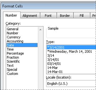
In the Type list, click the date or time format that you want to use.
Note: Date and time formats that begin with an asterisk (*) respond to changes in regional date and time settings that are specified in Control Panel. Formats without an asterisk are not affected by Control Panel settings.
To display dates and times in the format of other languages, click the language setting that you want in the Locale (location) box.
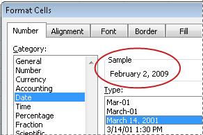
The number in the active cell of the selection on the worksheet appears in the Sample box so that you can preview the number formatting options that you selected.
Create a custom date or time format
On the Home tab, click the Dialog Box Launcher next to Number.
You can also press CTRL+1 to open the Format Cells dialog box.
In the Category box, click Date or Time, and then choose the number format that is closest in style to the one you want to create. (When creating custom number formats, it’s easier to start from an existing format than it is to start from scratch.)
In the Category box, click Custom. In the Type box, you should see the format code matching the date or time format you selected in the step 3. The built-in date or time format can’t be changed or deleted, so don’t worry about overwriting it.
In the Type box, make the necessary changes to the format. You can use any of the codes in the following tables:
Days, months, and years
Months as Jan–Dec
Months as January–December
Months as the first letter of the month
Days as Sunday–Saturday
Years as 1900–9999
If you use «m» immediately after the «h» or «hh» code or immediately before the «ss» code, Excel displays minutes instead of the month.
Hours, minutes, and seconds
Minutes as 00–59
Seconds as 00–59
Time as 4:36:03 P
Elapsed time in hours; for example, 25.02
Elapsed time in minutes; for example, 63:46
Elapsed time in seconds
Fractions of a second
AM and PM If the format contains an AM or PM, the hour is based on the 12-hour clock, where «AM» or «A» indicates times from midnight until noon and «PM» or «P» indicates times from noon until midnight. Otherwise, the hour is based on the 24-hour clock. The «m» or «mm» code must appear immediately after the «h» or «hh» code or immediately before the «ss» code; otherwise, Excel displays the month instead of minutes.
Creating custom number formats can be tricky if you haven’t done it before. For more information about how to create custom number formats, see Create or delete a custom number format.
Tips for displaying dates or times
To quickly use the default date or time format, click the cell that contains the date or time, and then press CTRL+SHIFT+# or CTRL+SHIFT+@.
If a cell displays ##### after you apply date or time formatting to it, the cell probably isn’t wide enough to display the data. To expand the column width, double-click the right boundary of the column containing the cells. This automatically resizes the column to fit the number. You can also drag the right boundary until the columns are the size you want.
When you try to undo a date or time format by selecting General in the Category list, Excel displays a number code. When you enter a date or time again, Excel displays the default date or time format. To enter a specific date or time format, such as January 2010, you can format it as text by selecting Text in the Category list.
To quickly enter the current date in your worksheet, select any empty cell, and then press CTRL+; (semicolon), and then press ENTER, if necessary. To insert a date that will update to the current date each time you reopen a worksheet or recalculate a formula, type =TODAY() in an empty cell, and then press ENTER.
Need more help?
You can always ask an expert in the Excel Tech Community or get support in the Answers community.
Источник
Insert the current date and time in a cell
Let’s say that you want to easily enter the current date and time while making a time log of activities. Or perhaps you want to display the current date and time automatically in a cell every time formulas are recalculated. There are several ways to insert the current date and time in a cell.
Insert a static date or time into an Excel cell
A static value in a worksheet is one that doesn’t change when the worksheet is recalculated or opened. When you press a key combination such as Ctrl+; to insert the current date in a cell, Excel “takes a snapshot” of the current date and then inserts the date in the cell. Because that cell’s value doesn’t change, it’s considered static.
On a worksheet, select the cell into which you want to insert the current date or time.
Do one of the following:
To insert the current date, press Ctrl+; (semi-colon).
To insert the current time, press Ctrl+Shift+; (semi-colon).
To insert the current date and time, press Ctrl+; (semi-colon), then press Space, and then press Ctrl+Shift+; (semi-colon).
Change the date or time format
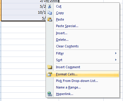
To change the date or time format, right-click on a cell, and select Format Cells. Then, on the Format Cells dialog box, in the Number tab, under Category, click Date or Time and in the Type list, select a type, and click OK.
Insert a static date or time into an Excel cell
A static value in a worksheet is one that doesn’t change when the worksheet is recalculated or opened. When you press a key combination such as Ctrl+; to insert the current date in a cell, Excel “takes a snapshot” of the current date and then inserts the date in the cell. Because that cell’s value doesn’t change, it’s considered static.
On a worksheet, select the cell into which you want to insert the current date or time.
Do one of the following:
To insert the current date, press Ctrl+; (semi-colon).
To insert the current time, press  + ; (semi-colon).
To insert the current date and time, press Ctrl+; (semi-colon), then press Space, and then press + ; (semi-colon).
Change the date or time format
To change the date or time format, right-click on a cell, and select Format Cells. Then, on the Format Cells dialog box, in the Number tab, under Category, click Date or Time and in the Type list, select a type, and click OK.
Insert a static date or time into an Excel cell
A static value in a worksheet is one that doesn’t change when the worksheet is recalculated or opened. When you press a key combination such as Ctrl+; to insert the current date in a cell, Excel “takes a snapshot” of the current date and then inserts the date in the cell. Because that cell’s value doesn’t change, it’s considered static.
On a worksheet, select the cell into which you want to insert the current date or time.
Do one of the following:
To insert the date, type the date (like 2/2), and then click Home > Number Format dropdown (in the Number tab) > Short Date or Long Date.
To insert the time, type the time, and then click Home > Number Format dropdown (in the Number tab) > Time.
Change the date or time format
To change the date or time format, right-click on a cell, and select Number Format. Then, on the Number Format dialog box, under Category, click Date or Time and in the Type list, select a type, and click OK.
Insert a date or time whose value is updated
A date or time that updates when the worksheet is recalculated or the workbook is opened is considered “dynamic” instead of static. In a worksheet, the most common way to return a dynamic date or time in a cell is by using a worksheet function.
To insert the current date or time so that it is updatable, use the TODAY and NOW functions, as shown in the following example. For more information about how to use these functions, see TODAY function and NOW function.
Current date (varies)
Current date and time (varies)
Select the text in the table shown above, and then press Ctrl+C.
In the blank worksheet, click once in cell A1, and then press Ctrl+V. If you are working in Excel for the web, repeat copying and pasting for each cell in the example.
Important: For the example to work properly, you must paste it into cell A1 of the worksheet.
To switch between viewing the results and viewing the formulas that return the results, press Ctrl+` (grave accent), or on the Formulas tab, in the Formula Auditing group, click the Show Formulas button.
After you copy the example to a blank worksheet, you can adapt it to suit your needs.
Note: The results of the TODAY and NOW functions change only when the worksheet is calculated or when a macro that contains the function is run. Cells that contain these functions are not updated continuously. The date and time that are used are taken from the computer’s system clock.
Need more help?
You can always ask an expert in the Excel Tech Community or get support in the Answers community.
Источник
Change the date system, format, or two-digit year interpretation
Dates are often a critical part of data analysis. You often ask questions such as: when was a product purchased, how long will a task in a project take, or what is the average revenue for a fiscal quarter? Entering dates correctly is essential to ensuring accurate results. But formatting dates so that they are easy to understand is equally important to ensuring correct interpretation of those results.
Important: Because the rules that govern the way that any calculation program interprets dates are complex, you should be as specific as possible about dates whenever you enter them. This will produce the highest level of accuracy in your date calculations.
Excel stores dates as sequential numbers that are called serial values. For example, in Excel for Windows, January 1, 1900 is serial number 1, and January 1, 2008 is serial number 39448 because it is 39,448 days after January 1, 1900.
Excel stores times as decimal fractions because time is considered a portion of a day. The decimal number is a value ranging from 0 (zero) to 0.99999999, representing the times from 0:00:00 (12:00:00 A.M.) to 23:59:59 (11:59:59 P.M.).
Because dates and times are values, they can be added, subtracted, and included in other calculations. You can view a date as a serial value and a time as a decimal fraction by changing the format of the cell that contains the date or time to General format.
Both Excel for Mac and Excel for Windows support the 1900 and 1904 date systems. The default date system for Excel for Windows is 1900; and the default date system for Excel for Mac is 1904.
Originally, Excel for Windows was based on the 1900 date system, because it enabled better compatibility with other spreadsheet programs that were designed to run under MS-DOS and Microsoft Windows, and therefore it became the default date system. Originally, Excel for Mac was based on the 1904 date system, because it enabled better compatibility with early Macintosh computers that did not support dates before January 2, 1904, and therefore it became the default date system.
The following table shows the first date and the last date for each date system and the serial value associated with each date.
January 1, 1900
(serial value 1)
December 31, 9999
(serial value 2958465)
January 2, 1904
(serial value 1)
December 31, 9999
(serial value 2957003)
Because the two date systems use different starting days, the same date is represented by different serial values in each date system. For example, July 5, 2007 can have two different serial values, depending on the date system that is used.
Serial value of July 5, 2007
The difference between the two date systems is 1,462 days; that is, the serial value of a date in the 1900 date system is always 1,462 days greater than the serial value of the same date in the 1904 date system. Conversely, the serial value of a date in the 1904 date system is always 1,462 days less than the serial value of the same date in the 1900 date system. 1,462 days is equal to four years and one day (which includes one leap day).
Important: To ensure that year values are interpreted as you intended, type year values as four digits (for example, 2001, not 01). By entering four-digit years, Excel won’t interpret the century for you.
If you enter a date with a two-digit year in a text formatted cell or as a text argument in a function, such as =YEAR(«1/1/31»), Excel interprets the year as follows:
00 through 29 is interpreted as the years 2000 through 2029. For example, if you type the date 5/28/19, Excel assumes the date is May 28, 2019.
30 through 99 is interpreted as the years 1930 through 1999. For example, if you type the date 5/28/98, Excel assumes the date is May 28, 1998.
In Microsoft Windows, you can change the way two-digit years are interpreted for all Windows programs that you have installed.
In the search box on the taskbar, type control panel, and then select Control Panel.
Under Clock, Language and Region, click Change date, time, or number formats
Click Regional and Language Options.
In the Region dialog box, click Additional settings.
Click the Date tab.
In the When a two-digit year is entered, interpret it as a year between box, change the upper limit for the century.
As you change the upper-limit year, the lower-limit year automatically changes.
Swipe in from the right edge of the screen, tap Search (or if you’re using a mouse, point to the upper-right corner of the screen, move the mouse pointer down, and then click Search), enter Control Panel in the search box, and then tap or click Control Panel.
Under Clock, Language and Region, click Change date, time, or number formats.
In the Region dialog box, click Additional settings.
Click the Date tab.
In the When a two-digit year is entered, interpret it as a year between box, change the upper limit for the century.
As you change the upper-limit year, the lower-limit year automatically changes.
Click the Start button, and then click Control Panel.
Click Region and Language.
In the Region dialog box, click Additional settings.
Click the Date tab.
In the When a two-digit year is entered, interpret it as a year between box, change the upper limit for the century.
As you change the upper-limit year, the lower-limit year automatically changes.
By default, as you enter dates in a workbook, the dates are formatted to display two-digit years. When you change the default date format to a different format by using this procedure, the display of dates that were previously entered in your workbook will change to the new format as long as the dates haven’t been formatted by using the Format Cells dialog box (On the Home tab, in the Number group, click the Dialog Box Launcher).
In the search box on the taskbar, type control panel, and then select Control Panel.
Under Clock, Language and Region, click Change date, time, or number formats
Click Regional and Language Options.
In the Region dialog box, click Additional settings.
Click the Date tab.
In the Short date format list, click a format that uses four digits for the year («yyyy»).
Swipe in from the right edge of the screen, tap Search (or if you’re using a mouse, point to the upper-right corner of the screen, move the mouse pointer down, and then click Search), enter Control Panel in the search box, and then tap or click Control Panel.
Under Clock, Language and Region, click Change date, time, or number formats.
In the Region dialog box, click Additional settings.
Click the Date tab.
In the Short date format list, click a format that uses four digits for the year («yyyy»).
Click the Start button, and then click Control Panel.
Click Region and Language.
In the Region dialog box, click Additional settings.
Click the Date tab.
In the Short date format list, click a format that uses four digits for the year («yyyy»).
The date system changes automatically when you open a document from another platform. For example, if you are working in Excel and you open a document that was created in Excel for Mac, the 1904 date system check box is selected automatically.
You can change the date system by doing the following:
Click File > Options > Advanced.
Under the When calculating this workbook section, select the workbook that you want, and then select or clear the Use 1904 date system check box.
You can encounter problems when you copy and paste dates or when you create external references between workbooks based on the two different date systems. Dates can appear four years and one day earlier or later than the date that you expect. You can encounter these problems whether you are using Excel for Windows, Excel for Mac, or both.
For example, if you copy the date July 5, 2007 from a workbook that uses the 1900 date system and then paste the date into a workbook that uses the 1904 date system, the date appears as July 6, 2011, which is 1,462 days later. Alternatively, if you copy the date July 5, 2007 from a workbook that uses the 1904 date system and then paste the date into a workbook that uses the 1900 date system, the date appears as July 4, 2003, which is 1,462 days earlier. For background information, see Date systems in Excel.
Correct a copy and paste problem
In an empty cell, enter the value 1462.
Select that cell, and then on the Home tab, in the Clipboard group, click Copy.
Select all of the cells that contain the incorrect dates.
Tip: To cancel a selection of cells, click any cell on the worksheet. For more information, see Select cells, ranges, rows, or columns on a worksheet.
On the Home tab, in the Clipboard group, click Paste, and then click Paste Special.

In the Paste Special dialog box, under Paste, click Values, and then under Operation, do one of the following:
To set the date as four years and one day later, click Add.
To set the date as four years and one day earlier, click Subtract.
Correct an external reference problem
If you are using an external reference to a date in another workbook with a different date system, you can modify the external reference by doing one of the following:
To set the date as four years and one day later, add 1,462 to it. For example:
To set the date as four years and one day earlier, subtract 1,462 from it. For example:
Need more help?
You can always ask an expert in the Excel Tech Community or get support in the Answers community.
Источник
In this guide, we’ll learn how to change date format in Excel. Date and Time data is an integral part of any statistical document or sheet. It is important to accurately track and analyze events, sales, figures, and others.
By convention, Excel uses a general data format that may be as per your need. But in most cases, that format may need to be customized.
Changing the format of Date in a particular cell or all the cells in your Excel sheet is an easy process and doesn’t require any complex methodologies. Excel provides a wide range of formatting options based on Location and Languages which helps in better date formatting in native language and style. Also, For some Languages there is also features to select from different Calendar types.
Follow the below step-by-step tutorial to change date format in Excel quickly and easily.
Step 1. Select the range of cells containing the date
To start with, select the cell values where want to change the date format, as shown in the image below.

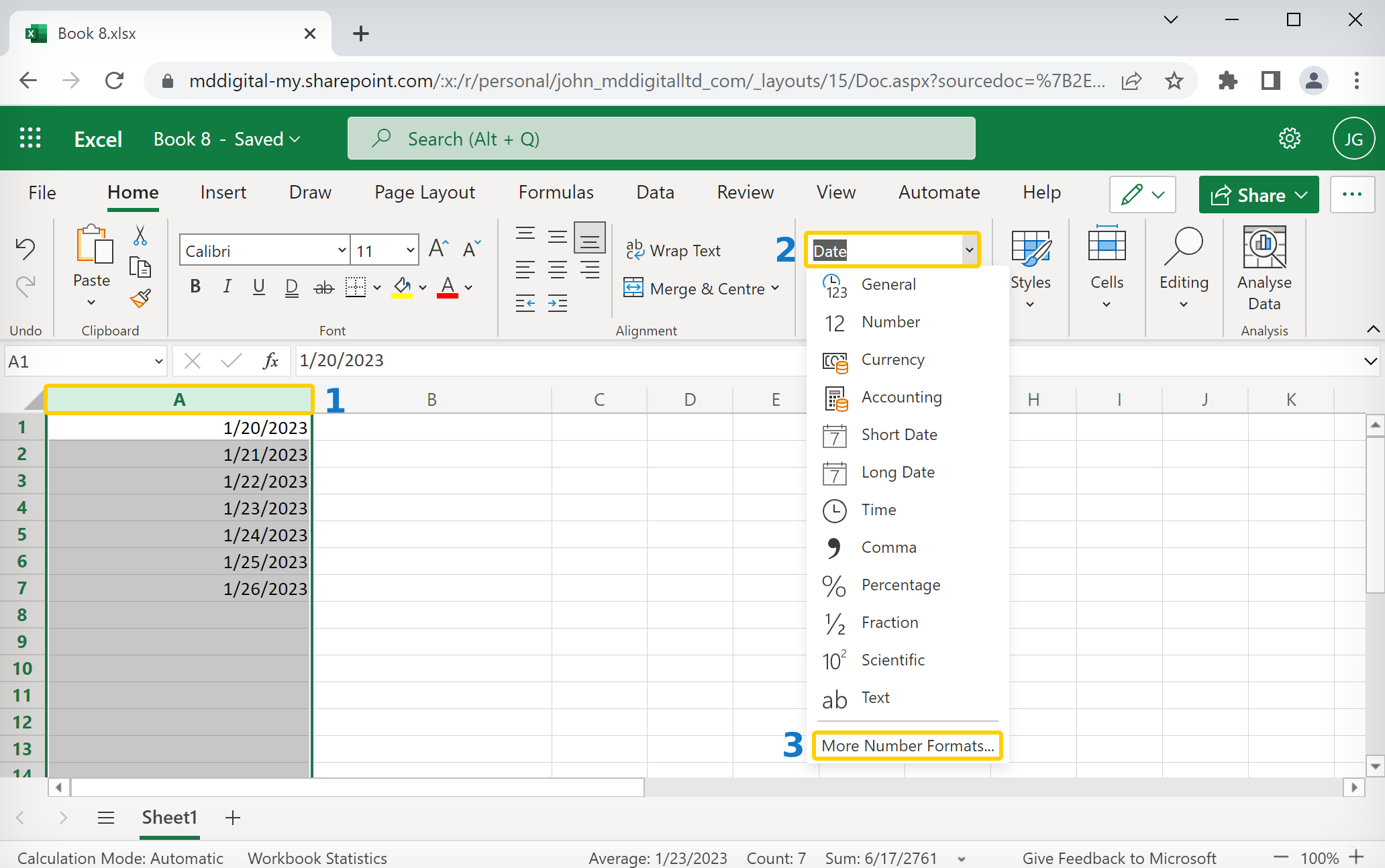
Step 2. Go to Number Format dropdown
- To select ‘Number Format’, go to ‘Home‘ in the option menu and look for Number Format, as shown below
- Then from the drop-down menu, select ‘More Number Formats‘ to reveal the ‘Number Format’ dialogue menu.

- Alternatively, you may directly go to Number Format, by right-clicking on the selected cell/s
- Click on ‘Number Format’.

Step 3. Choose Date
- From the Category menu on the right, choose ‘Date‘.

Now, to apply any date formatting type, select it from the right panel of the pop-up menu of Number Format. Click on ‘OK‘ to apply the formatting to the selected cell/s.
Note: You may check the date format implementation in the ‘Sample‘ at the top of the menu option
Choose the Date Type
The general option type to choose from a variety of Date Formatting options. Scroll down in this section to reveal a plethora of options for formatting, ranging from date, text (month name), year, and others.
This option can be perceived as the display menu, as the formatting options in this will keep on changing as per the selection in Locale(Location) and Calendar type.

Choose the Locale (location)
This option features the Location or Language options to help format the date accordingly. This option is probably the most used option as users require to format the date according to their or audience preference as per the native formatting style, based on language and location.
Choose any language or Location from this options menu. After selecting, all the supported date format options available for that particular locale will be available for selecting in the above Type menu.

Choose the type of calendar
This option reveals different calendar types available based on the Locale(Location) selected from the above option menu. This formatting option is only available for certain Locale and not all.
As shown in our example below, the variety of calendar types available for selection are only available for the Locale (location) selected (here, Arabia), for other locales the calendar type might be different or not at all present.

To apply selected formatting, you will need to click ‘OK‘ after selection to apply to your dates.
Conclusion
That’s It! You can now easily convert your dates to your desired format style easily.
We hope you learned and enjoyed this lesson and we’ll be back soon with another awesome Excel tutorial at QuickExcel!
This article will explain to you how to change the default Date format by your custom display.
How is displayed a date in Excel?
By default, when you insert a date in a cell, the default delimiter between the day, the month and the year it’s the slash. And this, even if you write your date with dashes.
Excel automatically replaces the dashes with slashes 🤔

Change the default Date format
If you want to customize the default display, you must change a Windows setting.
Step 1: Open the Regional setting
To open the Regional setting quickly, you write the command line intl.cpl in the Windows Search box

And there, you have the following dialog box with the default date format.

Step 2: Select another date format
When you press on the drop-down button, you display other date formats but the number of choices is limited 😕

Step 3: Change the default date format
To change the default date format, you must click on the button Additional Settings

Step 4: Create your custom date format
- Select the Date tab
- Change the custom date format (here dd-MM-yyyy)

The code of your custom date follow the standard rules of date format in Excel
And without restarting Excel, neither your computer, all the dates format in your worksheets has the dash for date delimiter 😉

Caution
When you change the setting of the date format of Windows, ALL THE DATES of your computer are impacted.
As you can see, after changing the default date format, the format of the date in the taskbar has changed too.

When you enter a date into Microsoft Excel, the program will format it according to the default date settings. For example, if you want to enter the date February 6, 2020, the date could appear as 6-Feb, February 6, 2020, 6 February, or 02/06/2020, all depending on your settings. You may find that if you change a cell’s formatting to “Standard,” your date becomes stored as integers. For example, February 6, 2020 would become 43865, because Excel bases date formatting off of January 1, 1900. Each of these options are ways to format dates in Excel. To help with organizing data in Excel, learn about how to change the date format in Excel.
Choosing from the Date Format List
Formatting dates in Excel is easiest with the date formats list. Most date formats you may want to use can be found in this menu.
How to Change The Excel Date Format
- Select the cells you want to format
- Click Ctrl+1 or Command+1
- Select the “Numbers” tab
- From the categories, choose “Date”
- From the “Type” menu, select the date format you want

Creating a Custom Excel Date Format Option
To customize the date format, follow the steps for choosing an option from the date format list. Once you’ve selected the closest date format to what you want, you can customize it and change it.
- In the “Category” menu, select “Custom”
- The type you chose earlier will appear. The changes you make will only apply to your customized setting, not to the default
- In the “Type” box, enter the correct code to alter the date
- If you are trying to change the date display to DD/MM/YYYY, simply go to Format Cells > Custom
- Next, Enter DD/MM/YYYY in the available space given.

Converting Date Formats to Other Locales
If you are using dates for several different locations, you might need to convert to a different locale:
- Select the right cell or cells
- Hit Ctrl+1 or Command+1
- From the “Numbers” menu, select “Date”
- Underneath the “Type” menu, there’s a drop-down menu for “Locale”
- Select the right “Locale”

You can also customize the locale settings:
- Follow the steps for customizing a date
- Once you’ve created the right date format, you need to add the locale code to the front of the customized date format
- Choose the right locale codes. All locale codes are formatted as [$-###]. Some examples include:
- [$-409]—English, United States
- [$-804]—Chinese, China
- [$-807]—German, Switzerland
- Find more locale codes

Tips for Displaying Dates in Excel
Once you have the right date format, there are additional tips to help you figure out how to organize data in Excel for your datasets.
- Make sure the cell is wide enough to fit the entire date. If the cell isn’t wide enough, it will display #####. Double click on the right border of the column to make your column expand enough to display the date correctly.
- Change the date system if negative numbers appear as dates. Sometimes Excel will format any negative numbers as a date because of the hyphens. To fix this, select the cells, open the options menu, and select “Advanced.” On that menu, select “Use 1904 date system.”
- Use functions to work with today’s date. If you want a cell to always display the current date, use the formula =TODAY() and press ENTER.
- Convert imported text to dates. If you import from an external database, Excel will automatically register the dates as text. The display may look the same as if they were formatted as dates, but Excel will treat the two differently. You can use the DATEVALUE function to convert.
Why Your Date Format May Not Be Having Issues Changing
There are many reasons why you might be experiencing issues changing the date format in Excel. Listed are a few common difficulties.
- There could be text in the column, not dates (which are actually numbers).
- Dates are left-aligned
- An apostrophe could be included in the date
- A cell may be too wide.
- Negative numbers are formatted as dates
- Excel TEXT function is not being utilized.
Even with correctly formatted dates and displays, organizing data in Excel can only work as well as the data does. Messy data won’t lead to insights during analysis, however, it’s formatted.
Data Preparation with Excel
Formatting data, by doing things like formatting dates, is part of a larger process known as “data preparation,” or all of the steps required to clean, standardize, and prepare data for analytic use.
While data preparation is certainly possible in Excel, it becomes exponentially more difficult as analysts work with larger and more complex datasets. Instead, many of today’s analysts are investing in modern data preparation platforms like Designer Cloud to accelerate the overall data preparation process for data big or small.
Schedule a demo of Designer Cloud to see how it can improve your data preparation process, or try the platform for yourself by getting started with Designer Cloud today.
If you are storing dates in Excel worksheets, the default format picked by the Excel is the format set in Control Panel. So, if your control panel setting is “M/d/yyyy”, the Excel will format the 2nd Feb 2010 date as follows:
2/2/2010
If you require displaying the date like 2-Feb-2010 or August 1, 2015, etc. as entering dates you may change the settings in Excel easily.
In case you require permanently changing the date format that applies to current as well as future work in Excel, you should change this in the control panel.
If you try entering a date like this: 20/2/2010 then Excel will take it as text because you provided day first for the default M/d/yyyy format.
For the current worksheet, you may set the date formatting in different ways as described in the following section with examples.
Related Learning: Add / Subtract Dates in Excel
First Way: Change the date format by “Format Cell” option
The first way I am going to show you for changing the date format in Excel is using the “Format Cells” option. Follow these steps:
Step 1:
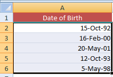
Right click on a cell or multiple cells where you require changing the date format. For the demo, I have entered a few dates and selected all:
Click the “Format Cells” option that should open the Format Cells dialog. You may also press the Ctrl+1 for opening this dialog in Windows. For Mac, the short key is Control+1 or Command+1.
Step 2:
In the Format Cells dialog, the Number tab should be pre-selected. If not, press Number tab. Under the Category, select Date. Towards the right side, you can see Type.
For the demo, I have selected 14-Mar-01 format and press OK. The resultant sheet after modifying date format is:
You are done!
An example of Mon-year format
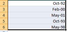
The following example displays the dates in Mon-Year format e.g. Oct-92. For that, open the “Format Cells” dialog again –> Number –> Date and select Mar-01 format.
The above sheet displays the same dates as shown below:
Similarly, you may choose any date format as per the requirement of your scenario.
Interesting Topic: How to calculate age in Excel
Change date format by locale/location
If you wish to display the dates based on other languages then you may use the Locale (location) option in the “Format Cells” dialog.
See the following Excel sheet where I set the Arabic(UAE) option and one of its type:
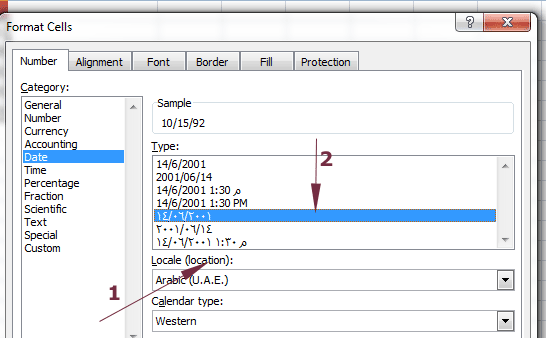
The resultant sheet for the same dates as in the above examples:
Similarly, you may choose the following locale:
- Bashkir (Russia)
- Chinese (Simplified, Singapore)
- Corsican (France)
- Danish (Denmark)
- Various options for English
- Hindi (India)
- Japanese (Japan)
- And many more
Customizing the date format
By using the date formatting codes, you may customize the dates in a flexible way. For example, displaying the short month name (Jan, Feb) by using “mmm” or full month name by “mmmm”.
Similarly, showing the day names of the Week (Sun, Mon) by ddd or full names (Sunday, Monday) by dddd formatting code.
First, have look at an example of customizing the date which is followed by the list of date formatting codes.
Select and right click on date cells that you want to customize and go to “Format Cells”. Under the Number –> Category, select Date and choose the closest format you wish to display e.g. “Mar 14, 2001”.
Under the Category, press Custom now and towards the right side, you should see Type with various options. Either choose a format from the available list or enter the formatting code as required in the text box under Type.
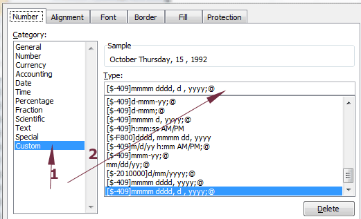
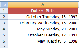
For the example, I entered the “[$-409]mmmm dddd, d , yyyy;@” and see the resultant sheet:
List of formatting codes in Excel
Following is the formatting code list that you may use to customize the dates:
Day Codes
- d – for the day as 1-31
- dd – for the day as 01-31
- ddd – Sun, Mon, Tue
- dddd – Sunday, Monday, Tuesday etc.
Month Codes
- m – for Months as 1-12
- mm – 01-12
- mmm – Apr, May, Jun etc.
- mmmm – April, May, June, July etc.
- mmmmm – Month as the first letter of the month
Year Codes
- yy – 00-99
- yyyy – 2000, 2002, 2010 etc.
You may also want to learn: Convert Number and Date to Text
Quick way of displaying dates in default short and long formats
If you need to display dates in the short or long format with default settings, you may do it by following this:
Select the dates you wish to format in short/long date formats. For that, I chose the above example dates that were formatted in the custom format (see the last graphic):
Now, go to the Home tab and in the Number group, click the Number Format box as shown below:
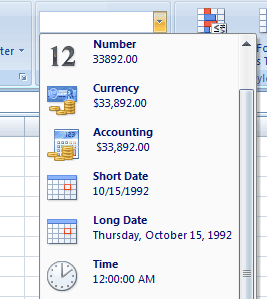
Press the Short Date or Long Date format.
Changing date format in Excel by TEXT function
The Excel TEXT function can also be used for formatting dates. The TEXT function takes two arguments as shown below:
=TEXT(Value to convert into text, “Formatting code “)
Where the first argument can be a date cell, a number etc.
The second argument should sound familiar now; the formatting code that we just learned.
The TEXT function for formatting dates can particularly be useful if you want to keep the original date column in place and displaying another date-set based on those dates.
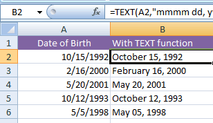
An example of Full month, day and year formatting example
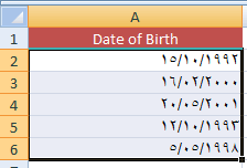
For the example, the A column cells are assigned the Date of Birth dates in default format (US English) i.e. M/d/yyyy.
The corresponding B cells will display the dates in full month name, day and year in four digits format.
The TEXT formula:
=TEXT(A2,«mmmm dd, yyyy»)
The resultant sheet with formatted dates:
I have written the formula in the B2 cell only and copied to B6 cell as follows.
After you get the result in B2 cell by writing the above formula, bring the mouse over the right bottom of the B2 cell. As + sign appears with solid line, drag the handle till B6 and formula should be copied to other cells. The Excel will update the corresponding A cells with respect to B cells automatically.
How to use the DATEDIF function in Excel
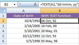
Formatting dates in d, mmm, yy by TEXT function
The following example displays the dates in day with leading zero (01-12), short month name and year in two-digit format.
The TEXT formula:
The resultant sheet:
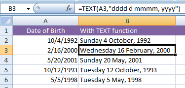
Displaying the day name as well
See the example below where day name (Sunday, Monday etc.) is also displayed along with day without leading zero, full month name and year in four digits.
The formula:
=TEXT(A2,«dddd d mmmm, yyyy»)
The dates after formatting:
The TEXT function is more than formatting dates; this is just one usage that I explained in above section. You may learn more about this function: The TEXT function in Excel
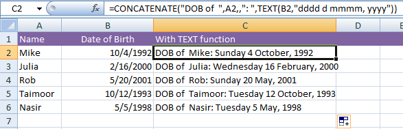
The example of concatenating formatted dates
Let us get more comfortable with date formatting and create more useful text strings as a result of joining different cells with constant literals.
In the example below, column A contains Names and column B date of births. In column C, I will use the CONCATENATE function where a text string is used and corresponding A and B cells are joined in the formula as follows:
=CONCATENATE(«DOB of «,A2,,«: «,TEXT(B2,«dddd d mmmm, yyyy»))
This is what we get:
Formatting dates specific to language by TEXT function
As we have seen in the custom date formatting example, you can display Locale specific date style. I showed an example of displaying dates in Arabic style by using custom date option in “Format cells” dialog.
You may also specify the language code in the TEXT function for displaying dates based on locales.
See the following example where I displayed dates in various languages by using TEXT function.
The resultant sheet:
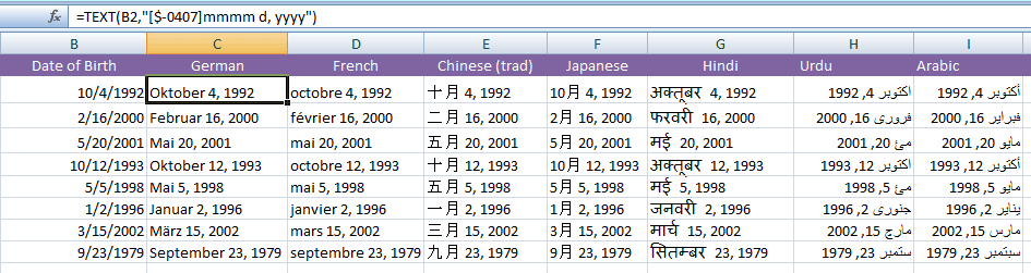
The following formulas are used for different languages:
For German:
=TEXT(B2,«[$-0407]mmmm d, yyyy»)
French:
=TEXT(B2,«[$-0040C]mmmm d, yyyy»)
Chinese (Traditional):
=TEXT(B2,«[$-0804]mmmm d, yyyy»)
Japanese:
=TEXT(B2,«[$-0411]mmmm d, yyyy»)
Arabic:
=TEXT(B2,«[$-0401]mmmm d, yyyy»)
For Hindi:
=TEXT(B2,«[$-0439]mmmm d, yyyy»)
Urdu:
=TEXT(B2,«[$-0420]mmmm d, yyyy»)
List of language codes
Following is the list of language codes that you may use in the TEXT function for locale-specific date formatting:
Lang. Code Language
- 042B Armenian
- 044D Assamese
- 082C Azeri (Cyrillic)
- 042C Azeri (Latin)
- 042D Basque
- 0423 Belarusian
- 0445 Bengali
- 0402 Bulgarian
- 0804 Chinese (Simplified)
- 0404 Chinese (Traditional)
- 041A Croatian
- 0405 Czech
- 0406 Danish
- 0413 Dutch
- 0C09 English (Australian)
- 1009 English (Canadian)
- 0809 English (U.K.)
- 0409 English (U.S.)
- 0464 Filipino
- 040B Finnish
- 040C French
- 0C0C French (Canadian)
- 0462 Frisian
- 0467 Fulfulde
- 0456 Galician
- 0437 Georgian
- 0407 German
- 0C07 German (Austrian)
- 0807 German (Swiss)
- 0408 Greek
- 0447 Gujarati
- 040D Hebrew
- 0439 Hindi
- 040E Hungarian
- 0421 Indonesian
- 0410 Italian
- 0411 Japanese
- 044B Kannada
- 0460 Kashmiri (Arabic)
- 0412 Korean
- 0476 Latin
- 0426 Latvian
- 0427 Lithuanian
- 042F Macedonian FYROM
- 043E Malay
- 044C Malayalam
- 043A Maltese
- 0458 Manipuri
- 044E Marathi
- 0450 Mongolian
- 0461 Nepali
- 0414 Norwegian Bokmal
- 0463 Pashto
- 0429 Persian
- 0415 Polish
- 0416 Portuguese (Brazil)
- 0816 Portuguese (Portugal)
- 0446 Punjabi
- 0418 Romanian
- 0419 Russian
- 044F Sanskrit
- 0C1A Serbian (Cyrillic)
- 081A Serbian (Latin)
- 0459 Sindhi
- 045B Sinhalese
- 041B Slovak
- 0424 Slovenian
- 0477 Somali
- 0C0A Spanish
- 0441 Swahili
- 041D Swedish
- 045A Syriac
- 0428 Tajik
- 045F Tamazight (Arabic)
- 085F Tamazight (Latin)
- 0449 Tamil
- 044A Telugu
- 041E Thai
- 041F Turkish
- 0442 Turkmen
- 0422 Ukrainian
- 0420 Urdu
- 0843 Uzbek (Cyrillic)
- 0443 Uzbek (Latin)
- 042A Vietnamese
- 0478 Yi
- 046A Yoruba
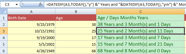
The example of calculating age in Years/Months and days
The following example uses the DATEDIF function for calculating the difference between current date and date of birth.
The current date is retrieved by using the TODAY() function. The Birth Date is stored in A column. The C column displays the formatted age in years, months and number of days.
The DATEDIF formula:
=DATEDIF(A3,TODAY(),«y») &» Years and «&DATEDIF(A3,TODAY(),«ym») &» Month(s) and « &DATEDIF(A3,TODAY(),«md») &» Days»
The resultant sheet:
For learning about the DATEDIF function, visit this tutorial: Excel DATEDIF function and formulas.
How to change date format in Excel 365 Online
Are you having a problem with date formatting in Excel 365 online? For example, are you finding your dates are showing as an American date format of mm/dd/yyyy or maybe the opposite with a UK date format of dd/mm/yyyy?
In this blog I’ll take you through a few things you can check in Excel 365 Desktop and Excel 365 Online so that you can change your date format to the Excel date format you require.
Why is the Excel 365 Online date format not working?
You may be experiencing problems within your own files, files you share with others, or both.
Saving files into OneDrive or SharePoint is a fantastic way for team members to be updating and working with files from outside of the office, and an excellent way for everyone to have access to the same file either inside or outside of the office.
However, it can be super frustrating when data is entered incorrectly as this impacts everyone using the file, and fixing formatting problems can be such a waste of your precious time.
Different date formats
Our client’s team had a problem with date formatting in Excel 365 Online when some members were updating dates in a shared file in the Desktop version of Excel 365, and others were updating dates in the same file using Excel 365 online, the web browser version.
Some team members were using both Excel 365 for Desktop when working in the office, and Excel 365 Online when working from home.
When dates were entered using Excel 365 desktop the date format was correct.
Sadly, the date formats kept changing when anyone accessing the file using Excel 365 online updated the file.
The team continually battled with dates entered as mm/dd/yyyy when they would normally use the dd/mm/yyyy format.
Additionally, some dates were aligned to the left of the cell and some to the right and this was happening in both the desktop and web versions of Excel.
This is how we fixed it.
Tip #1 Check the Date format in Excel Desktop
The first thing we checked was the date formatting had been set correctly as dd/mm/yyyy in Excel 365 Desktop.
We work with a New Zealand date format of day/month/year, a.k.a dd/mm/yyyy, e.g. 31/01/2022.
Change the date format in Excel Desktop
1. To check the current date format first select the cell range containing the dates, and then right-click any cell in the selected range.
2. Click Format Cells.
3. On the Number tab click Date and then check that your date is set to the format you require. You can see in the image below that ours is set to dd/mm/yyyy and the Sample box shows the date as 31/01/2022 which is exactly how we are wanting it to be displayed.
Also, check that the Locale option is set to your location. Ours is set correctly with English (New Zealand).
Notes: if the Date format is set incorrectly here you can select the format you require from the Date options.
Additionally, if the date format is showing as an American date format, you can easily change the date format in Excel by selecting Custom from the Category group, and then changing the Excel date format to the format you require.
You can see in the image below that ours is set to dd/mm/yyyy and the Sample box shows the date as 31/01/2022 which is exactly how we are wanting it to be displayed for our New Zealand date format.
If you wanted month/day/year you could enter a new format into the Type box. For example, for an American date format you could type mm/dd/yyyy, as shown below.
Excel Online date format not working
We found that the date settings were set correctly in Excel 365 Desktop.
However, even if we clicked OK to reapply the formatting on every selected cell, we still had several cells that were still formatted incorrectly with the date still left-aligned in the column.
We used the steps in Tip #3 below to reset the dates to the correct format.
Additionally, as soon as a team member accessed the file using Excel 365 Online the dates went back to being formatted incorrectly.
We then tried the steps in Tip #2.
Tip #2 Change the date format in Excel 365 Online
When team members were editing the sheet in the browser version of Excel (Excel 365 Online) the formatting changed to month/day/year, a.k.a mm/dd/yyyy, even though the date formats were set correctly in Excel 365 Desktop.
This was the reason some of the dates were being left-aligned in the column. For example, 31/01/2022 was being entered incorrectly because the web version of Excel 365 was seeing the date as mm/dd/yyyy. Since there isn’t a 31st month, Excel saw this as a mistype and entered the date as text, not a date.
However, because the date format was set to read month then day, entering 01/02/2022 was being entered as a date but it was being held as the 2nd of January, not the 1st of February.
Change the Date Format in Excel 365 Online
We followed the same steps as for Excel 365 Desktop to check the current Excel date format. To do this follows these steps.
1. Login to your Excel 365 Online account and open the file.
2. Select the cell range containing the dates, and then right-click any cell in the selected range.
3. Click Number Format.
4. On the Custom option we can see that the date format is set to dd/mm/yyyy. However, the dates were still being formatted incorrectly.
Note: there isn’t currently a way to change the date format within the Custom area in Excel 365 Online. To do this you will need to open the file into Excel 365 Desktop and follow the steps outlined above.
5. Click Date in the Category list.
6. Now, this is the important part. Check the Locale (location) setting. We had such a mix of settings for this. Some members of the team had English (United States), while others had Armenian or Azerbaijani!
7. Now select the correct date format you require from the Type list.
8. Select your location from the Locale (location) list.
Note: please be aware that changing the Regional format settings in Excel affect dates, currency, formula delimiters and more. For more information, please check the Microsoft support page online.
9. BEFORE you click OK be sure to select the Set this locate as the preferred regional format option box. If you don’t do this the date format will change itself back to its former setting again.
10. When you click OK the file will update.
11. Once the new date format is in place all dd/mm/yyyy date entries will be formatted with the correct Excel date format. If you find existing date entries still haven’t updated, please check the steps in Tip #3 below.
Note: you can also change the Excel 365 Online Regional format settings through File, Options. To do this follow the steps below.
1. Click the File tab and then click the 3 dots for access the More File Options.
2. Select Options.
3. Now click Regional Format Settings.
4. Select your preferred regional format from the drop-down list and then click Change.
Tip #3 Change existing dates to the correct date format in Excel
The tips above will set your date format for all dates entered going forward.
However, you may now be left with existing dates that are still in the incorrect format.
Let’s look at a quick way to fix this.
1. Select the cells that need to be reformatted with the correct date format.
2. From the Data tab select Text to Columns.
3. Follow the instruction for the version of Excel you are working in.
Change existing dates in Excel 365 Online
Remove the selection from all the Delimiter options and then click Apply.
Change existing dates in Excel 365 for Desktop
1. On Step 1 of the Convert Text to Columns Wizard select Delimited and then click Next.
2. On Step 2, leave all the delimiter options unchecked and then click Next.
3. On Step 3, select Date from the Column data format option box, and then select the format that the date is currently using. For example, if your date format is currently mm/dd/yy, and you want to change it to your default locale setting, select MDY. If it is dd/mm/yy and you want the dates to be formatted as American date format select DMY.
4. Click Finish.
Your dates will now be updated and the correct Date Formats reapplied.
Was this blog helpful? Let us know in the Comments below.
Instructions
Change the date format in Excel Desktop
- Select the cell range containing the dates, and then right-click any cell in the selected range.
- Click Format Cells.
- On the Number tab click Date and then check that your date is set to the format you require. Also, check that the Locale option is set to your location.
Change the Date Format in Excel 365 Online
- Login to your Excel 365 Online account and open the file.
- Select the cell range containing the dates, and then right-click any cell in the selected range.
- Click Number Format.
- On the Custom option we can see that the date format is set to dd/mm/yyyy.
- Click Date in the Category list.
- Check the Locale (location) setting.
- Now select the correct date format you require from the Type list.
- Select your location from the Locale (location) list.
- BEFORE you click OK be sure to select the Set this locate as the preferred regional format option box. If you don’t do this the date format will change itself back to its former setting again.
- When you click OK the file will update.
Change existing dates to the correct date format in Excel
The tips above will set your date format for all dates entered going forward. However, you may now be left with existing dates that are still in the incorrect format. To fix this:
- Select the cells that need to be reformatted with the correct date format.
- From the Data tab select Text to Columns.
- Follow the instruction for the version of Excel you are working in.
Change existing dates in Excel 365 Online
Remove the selection from all the Delimiter options and then click Apply.
Change existing dates in Excel 365 for Desktop
- On Step 1 of the Convert Text to Columns Wizard select Delimited and then click Next.
- On Step 2, leave all the delimiter options unchecked and then click Next.
- On Step 3, select Date from the Column data format option box, and then select the format that the date is currently using. For example, if your date format is currently mm/dd/yy, and you want to change it to your default locale setting, select MDY. If it is dd/mm/yy and you want the dates to be formatted as American date format select DMY.
- Click Finish.
Notes
Why is the Excel 365 Online date format not working?
Different date formats: Our client’s team had a problem with date formatting in Excel 365 Online when some members were updating dates in a shared file in the Desktop version of Excel 365, and others were updating dates in the same file using Excel 365 online, the web browser version. The team continually battled with dates entered as mm/dd/yyyy when they would normally use the dd/mm/yyyy format.
Change the date format in Excel Desktop
Note: if the Date format is set incorrectly in the Format Cells display box you can select the format you require from the Date options. Additionally, if the date format is showing as an American date format, you can easily change the date format in Excel by selecting Custom from the Category group, and then changing the Excel date format to the format you require. If you wanted month/day/year you could enter a new format into the Type box. For example, for an American date format you could type mm/dd/yyyy.
Change the Date Format in Excel 365 Online
Note: there isn’t currently a way to change the date format within the Custom area in Excel 365 Online.
Note: please be aware that changing the Regional format settings in Excel affect dates, currency, formula delimiters and more.
Change the Excel 365 Online Regional Format settings
- Click the File tab and then click the 3 dots for access the More File Options.
- Select Options.
- Now click Regional Format Settings.
- Select your preferred regional format from the drop-down list and then click Change.
Elevate your Excel game and become a pro with our exclusive Insider Group.
Be the first to know about new tutorials, videos, and tips for Microsoft 365 products. Join us now and claim your exclusive bonus today!
The standard date format in the UK is different for the US. In the UK, dates are formatted dd/mm/yyyy (day/month/year), whereas in the US, dates are formatted mm/dd/yyyy (month/day/year). If you want to switch from one format to another, you can do that using the desktop and web versions of Microsoft Excel. And in this guide, we’ll show you how!
How to change the date format in Excel from mm/dd/yyyy to dd/mm/yyyy (desktop):
- Open your
 Excel desktop application.
 - Select the cell, row, or column that you want to change in your spreadsheet.
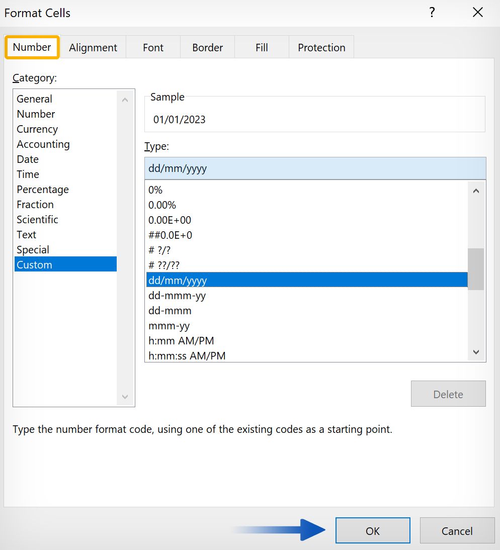
- Press Ctrl+1 or click “Home,” then click the
 pop out icon in the “Number” section.
 - Click on “Custom” at the bottom of the left menu.
- Select “dd/mm/yyyy” from the list.
- Click “OK.”
How to change the date format in Excel from mm/dd/yyyy to dd/mm/yyyy (web):
- Go to office.com and open Excel.
- Select the cell, row, or column that you want to change in your spreadsheet.
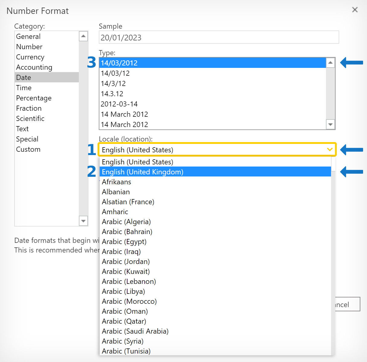
- Press Ctrl+1 or click “Home,” click the select box in the “Number” section, then select “More Number Formats” at the bottom of the list.
- Click the dropdown box under “Locale (Location).”
- Select “English (United Kingdom)” from the dropdown box.
- Then select “14/03/2012” from the “Type” list.
- Click “OK.”
Please continue reading for a detailed, step-by-step guide on changing the date format in Excel.
How are dates formatted in Excel?
Dates in Excel are referred to as “Serial numbers” and can be stored in long or short-form, as well as numeric values. A simple way to convert or format a date is to use the TEXT function. For example, the function =TEXT(A1, “dddd”) would return “Sunday” if the date in the “A1” cell was “01/01/2023.”
| Date / Time | Format | Result |
|---|---|---|
| 01/01/2023 | d | 1 |
| 01/01/2023 | dd | 01 |
| 01/01/2023 | ddd | Sun |
| 01/01/2023 | dddd | Sunday |
| 01/01/2023 | m | 1 |
| 01/01/2023 | mm | 01 |
| 01/01/2023 | mmm | Jan |
| 01/01/2023 | mmmm | January |
| 01/01/2023 | mmmmm | J |
| 01/01/2023 | y | 23 |
| 01/01/2023 | yy | 23 |
| 01/01/2023 | yyy | 2023 |
| 01/01/2023 | yyyy | 2023 |
| 1:05:06 AM | h | 1 |
| 1:05:06 AM | hh | 01 |
| 1:05:06 AM | h:m | 1:5 |
| 1:05:06 AM | h:mm | 1:05 |
| 1:05:06 AM | hh:mm | 01:05 |
| 1:05:06 AM | s | 6 |
| 1:05:06 AM | ss | 06 |
| 1:05:06 AM | hh:mm:ss AM/PM | 01:05:06 AM |
Method 1: Format dates using a custom format (Desktop)
To demonstrate this method, we’ve created a spreadsheet in Excel with a list of US-formatted dates. You can still follow along if the dates in your spreadsheet are listed differently. However, you will need the ![]() desktop version of Microsoft Excel for the steps below.
desktop version of Microsoft Excel for the steps below.
The same effect can be achieved in the web version of Excel using a slightly different process.
- First, open the desktop version of Excel and the workbook containing your dates.
- Then, select all the cells you want to format.
 Notes:
- A simple way to select cells is to click and drag over them.
- Alternatively, you can select the entire row or column.
- Or select individual cells by pressing Ctrl + click.
- Then, with your cells selected, press Ctrl + 1 on your keyboard.
- Alternatively, click on the pop out icon in the “Number” section in the “Home” tab.
- Next, click on “Custom” at the bottom of the left menu.
- Then select “dd/mm/yyyy” from the “Type” list.
- You can also manually type in the format of your choice into the text bar.
- Click “OK” to finish.
By formatting the whole column instead of individual rows, any additional dates entered into that column will be changed from mm/dd/yyyy to dd/mm/yyyy automatically. You can also use the same process to change a date from dd/mm/yyyy to mm/dd/yyyy. Please view the image below:
Method 2: How to change the date format in Excel from mm/dd/yyyy to dd/mm/yyyy using a custom format (Web)
- First, go to office.com and open Excel.
- Open the workbook containing your dates.
- Select the cells that you want to format.
- Notes:
- A simple way to select cells is to click and drag over them.
- Alternatively, you can select the entire row or column. (1)
- Or select individual cells by pressing Ctrl + click.
- With the cells selected, press Ctrl + 1.
- Alternatively, click the dropdown box in the “Number” section. (2)
- Then select “More Number Formats” at the bottom of the list. (3)
- Click the dropdown box under “Locale (Location).” (1)
- Select “English (United Kingdom)” from the dropdown box. (2)
- Then select “14/03/2012” from the “Type” list. (3)
- Click the “OK” button, and your dates will change from mm/dd/yyyy to dd/mm/yyyy.
- To reverse the process, select “English (United States)” as the location.
- Then select “*3/14/2012” from the “Type” list.
Method 3: How to change date format in Excel from mm/dd/yyyy to dd/mm/yyyy using a formula (Desktop & Web)
If you want to change an mm/dd date to a dd/mm date in the web version of Excel, you can do that by using the TEXT function. Please follow the steps below to learn how.
- First, go to office.com and open Excel, or open your Excel desktop application.
- Open your workbook and select an empty cell on the same row or adjacent to your date.
- Then, type the following formula into the cell:
=TEXT(CELL, "dd/mm/yyyy")Replace “CELL” with the cell address of your date (e.g., A1). If your dates are in a list, select an empty cell in the same row as the top date.
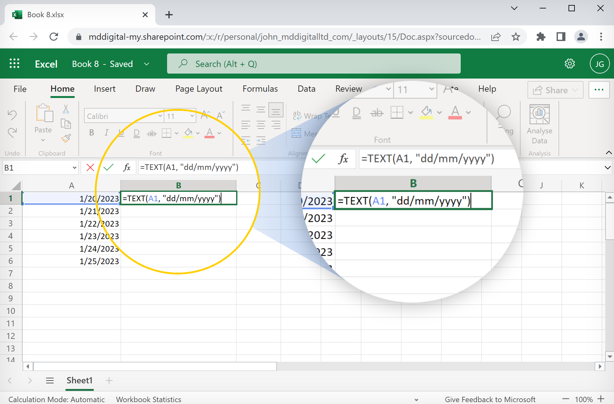
- Once you’ve typed in the formula, press the Enter key.
- Click the formula cell and hover over the corner until you see a black
 plus symbol.
 - Then click and drag the function down next to all your dates.
The dates in Column A will automatically appear in Column B with the format changed from the US standard (mm/dd/yyyy) to the UK standard (dd/mm/yyyy).
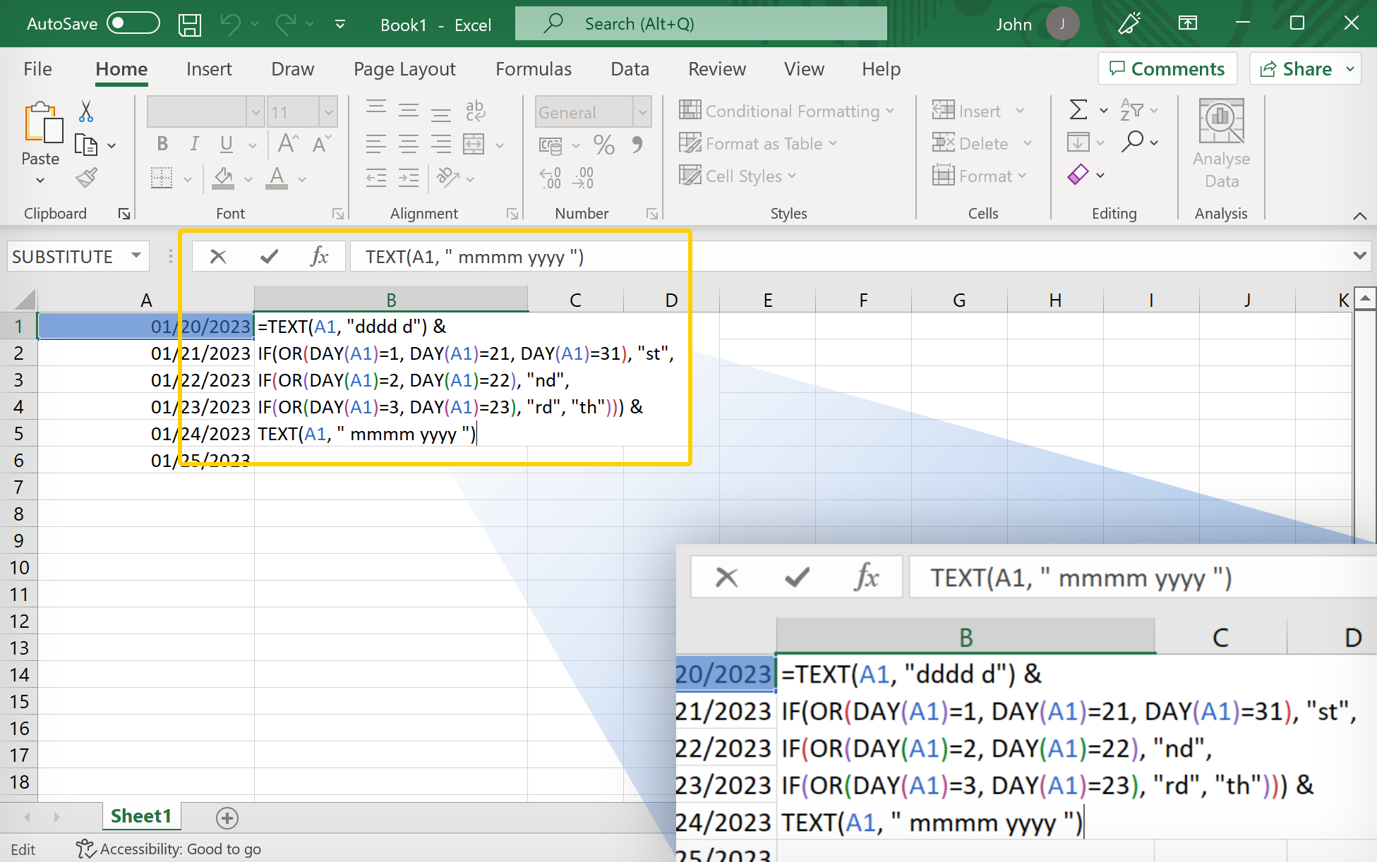
Method 4: Change the short date format to a long-form date in Excel with st, nd, and rd (Desktop & Web)
So far, we’ve covered how to convert an mm/dd date into a dd/mm date, but there are other interesting ways of formatting dates in Excel. You can’t add st, nd, and rd to the days of the month using a single function, but you can achieve that effect using a formula.
We’re going to turn “1/20/2023” into “Friday 20th January 2023.”
- First, go to office.com and open Excel, or open your Excel desktop application.
- Open your workbook and select an empty cell on the same row or adjacent to your date.
- Then, type the following formula into the cell:
=TEXT(CELL, "dddd d") &
IF(OR(DAY(CELL)=1, DAY(CELL)=21, DAY(CELL)=31), "st",
IF(OR(DAY(CELL)=2, DAY(CELL)=22), "nd",
IF(OR(DAY(CELL)=3, DAY(CELL)=23), "rd", "th"))) &
TEXT(CELL, " mmmm yyyy ")- Change “CELL” to the cell address (e.g., A1) where your first date is located.
- Then press the “Enter” key.
- Click the formula cell and hover over the corner until you see a black plus symbol.
- Then click and drag the function down next to all your dates.
The dates in Column A will automatically appear in Column B with the format changed from the US standard to a long format, including st, nd, and rd for the days of the month.
Conclusion
The best way to format mm/dd dates into dd/mm dates in Excel is to use Method 1 or 2, depending on whether you are using the desktop or web version. It would be ideal if your dates were listed in a single column, as you can format the whole column into dd/mm. That way, whenever you add a new date to the column, it will automatically change to the correct format.
Method 3 is ideal if you want to keep both the US (mm/dd) and UK (dd/mm) date formats in separate columns. But if you’re looking for readability, Method 4 is perfect!
Thank you for reading our guide.