
Create a simple formula in Excel
Excel for Microsoft 365 Excel for Microsoft 365 for Mac Excel 2021 Excel 2021 for Mac Excel 2019 Excel 2019 for Mac Excel 2016 Excel 2016 for Mac Excel 2013 Excel 2010 Excel 2007 Excel for Mac 2011 More…Less
You can create a simple formula to add, subtract, multiply or divide values in your worksheet. Simple formulas always start with an equal sign (=), followed by constants that are numeric values and calculation operators such as plus (+), minus (—), asterisk(*), or forward slash (/) signs.
Let’s take an example of a simple formula.
-
On the worksheet, click the cell in which you want to enter the formula.
-
Type the = (equal sign) followed by the constants and operators (up to 8192 characters) that you want to use in the calculation.
For our example, type =1+1.
Notes:
-
Instead of typing the constants into your formula, you can select the cells that contain the values that you want to use and enter the operators in between selecting cells.
-
Following the standard order of mathematical operations, multiplication and division is performed before addition and subtraction.
-
-
Press Enter (Windows) or Return (Mac).
Let’s take another variation of a simple formula. Type =5+2*3 in another cell and press Enter or Return. Excel multiplies the last two numbers and adds the first number to the result.
Use AutoSum
You can use AutoSum to quickly sum a column or row or numbers. Select a cell next to the numbers you want to sum, click AutoSum on the Home tab, press Enter (Windows) or Return (Mac), and that’s it!
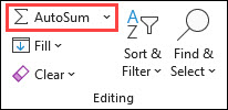
When you click AutoSum, Excel automatically enters a formula (that uses the SUM function) to sum the numbers.
Note: You can also type ALT+= (Windows) or ALT+ += (Mac) into a cell, and Excel automatically inserts the SUM function.
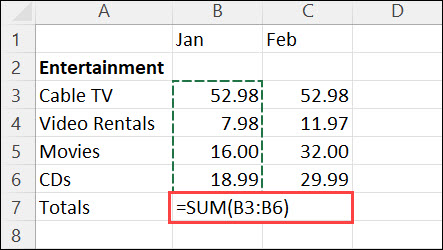
Here’s an example. To add the January numbers in this Entertainment budget, select cell B7, the cell immediately below the column of numbers. Then click AutoSum. A formula appears in cell B7, and Excel highlights the cells you’re totaling.
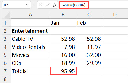
Press Enter to display the result (95.94) in cell B7. You can also see the formula in the formula bar at the top of the Excel window.
Notes:
-
To sum a column of numbers, select the cell immediately below the last number in the column. To sum a row of numbers, select the cell immediately to the right.
-
Once you create a formula, you can copy it to other cells instead of typing it over and over. For example, if you copy the formula in cell B7 to cell C7, the formula in C7 automatically adjusts to the new location, and calculates the numbers in C3:C6.
-
You can also use AutoSum on more than one cell at a time. For example, you could highlight both cell B7 and C7, click AutoSum, and total both columns at the same time.
Copy the example data in the following table, and paste it in cell A1 of a new Excel worksheet. If you need to, you can adjust the column widths to see all the data.
Note: For formulas to show results, select them, press F2, and then press Enter (Windows) or Return (Mac).
|
Data |
||
|
2 |
||
|
5 |
||
|
Formula |
Description |
Result |
|
=A2+A3 |
Adds the values in cells A1 and A2 |
=A2+A3 |
|
=A2-A3 |
Subtracts the value in cell A2 from the value in A1 |
=A2-A3 |
|
=A2/A3 |
Divides the value in cell A1 by the value in A2 |
=A2/A3 |
|
=A2*A3 |
Multiplies the value in cell A1 times the value in A2 |
=A2*A3 |
|
=A2^A3 |
Raises the value in cell A1 to the exponential value specified in A2 |
=A2^A3 |
|
Formula |
Description |
Result |
|
=5+2 |
Adds 5 and 2 |
=5+2 |
|
=5-2 |
Subtracts 2 from 5 |
=5-2 |
|
=5/2 |
Divides 5 by 2 |
=5/2 |
|
=5*2 |
Multiplies 5 times 2 |
=5*2 |
|
=5^2 |
Raises 5 to the 2nd power |
=5^2 |
Need more help?
You can always ask an expert in the Excel Tech Community or get support in the Answers community.
Need more help?
Want more options?
Explore subscription benefits, browse training courses, learn how to secure your device, and more.
Communities help you ask and answer questions, give feedback, and hear from experts with rich knowledge.

How to Create a Simple Formula in Excel
To create a formula in excel must start with the equal sign “=”. If there is no equals sign, then whatever is typed in the cell will not be regarded as a formula.
Here’s how to create a simple formula, which is a formula for addition, subtraction, multiplication, and division. An addition formula using the plus sign “+”, subtraction formula using the negative sign “-“, a multiplication formula using an asterisk sign “*” and division formula using the slash “/”.
Addition Formula
There are two numbers in cell B1 and B2. How to create a formula in excel to add both of them?

There are several ways of writing a formula. The first way is using the keyboard and the arrow keys, the second way using the keyboard and mouse and a third way to use the keyboard by typing directly the formula and the address of cell involved.
For the above addition, the formula will be used the first way.
- Place the cursor in cell B4 and then type the equals sign “=”

- Press the up arrow button, point to cell B1, the cursor turns into dashed line.

- Type the plus sign “+” for the addition operation

- Press the up arrow button again, point to cell B2

- Press the ENTER key
The result is as shown below

Subtraction Formula
How to write a formula in excel for subtracting number1 by number2?. The reduction formula to use the second way, i.e. using the keyboard and mouse.
- Place the cursor in cell B5 and then type the equals sign “=”
- Click cell B1 using the mouse
- Type the negative sign “-” for the subtraction operation
- Click cell B2 using the mouse
- Press the ENTER key
For more details, you can see the animation below.
Multiplication Formula
How to make a formula in excel to multiply number1 by number2. For the multiplication formula using the third way of using the keyboard by writing directly the formula and the address of the cell involved.
- Place the cursor in cell B6 and then type the equals sign “=”
- Type B1
- Type an asterisk “*” for multiplication operations
- Type B2
- Press the ENTER key
For more details, you can see the animation below.
Division Formula
How to do formulas in excel to divide number1 with number2.
- Place the cursor in cell B7 and then type the equals sign “=”
- Point the cursor to cell B1
- Type a slash mark “/” for the division operation
- Point the cursor to cell B2
- Press the ENTER key
The result is as shown below

How to View Formulas in Excel
The easiest way to see the formula in a cell is to look at the formula bar. Point the cursor to a cell that contains a formula, then the formula bar will display the formula in the cell. The location of the formula bar is below the ribbon menu.

The picture above shows the formula contained in cell B4. To see formulas in other cells just move the cursor to the desired cell and see the formula in the formula bar.
Formula bar can only display formulas in the active cell, meaning only one formula can be shown. To be able to display all the formulas in a worksheet, please read the article below “How to Display Cell Formulas in Excel”
How to Edit Formula in Excel
There are two ways to edit a formula, using the F2 key or using a formula bar.
Editing with the F2 key
Place the cursor in the cell containing the formula, then press the F2 key. The contents of the formula will appear, and the cells involved in the formula will be marked with a colored box.
The picture below shows the existing addition formula in cell B4. There are two cells involved in the formula: cell B1 and B2. The address of the cell B1 light blue colored then the cell B1 will be surrounded with the same colored line, likewise with cell B2, the color of lines around it is same as cell B2 address color.

For example, the formula will be edited by adding the number 2. Type the plus sign “+”, number 2 and then press the ENTER key.
The results are as shown below. The formula in cell B4 has changed.

Editing with the formula bar
Place the cursor in the cell containing the formula, then click on the formula bar section. The formula in the cell will appear automatically. The display will be the same as when pressing the F2 key.
The picture below shows the existing subtraction formula in cell B5. For example, the formula will be edited by subtracting the number 2. Type a negative sign “-” number 2, then press the ENTER key.
How to Copy Formula in Excel
The cell that contains the formula can be copied like any other data. The difference, which is copied is the formula, not the value of the cell and the cell address forming the formula will be changed according to the location.
See image below. Cell B4 contains a formula that adds the value of cell B1 and B2. The formula will be copied and placed in the range C4: F4.

Place the cursor in cell B4. Do a copy (CTRL + C). Select C4: F4 range, then paste it (CTRL + V).
The result is as shown below.

The value of cell C4 to F4 is not equal to the value of cell B4, because excel copied the formula, not the cell value. Cell C4 contains a formula that adds C1 and C2 values, as well as cell D4 until F4; all contain a formula that adds cell values in row 1 and row 2 in the same column.
Another way to copy formula in excel
In addition to using the keyboard, there is another way to copy the formula, which is using the mouse. Eg formula in cell B5 will be copied. Click cell B5, point mouse to bottom right of cell B5 until the cursor change shape become thinner. Click and hold, then drag the cursor until cell F5. The result is as shown below.
Is there any other way to copy the formula with the mouse, of course 😊. For example, the formula in range B6: B7 will be copied. Select range B6: B7, then right click select copy. Select range C6: F7, right click, select Paste. The result as shown below.
How to Paste Special in Excel
If the cell that contains the formula is copied, the formulas are copied, not its value. The question is what if you want to copy the value, not the formulas. The solution is using Paste Special.
For example, there are data like the image above. Range A4:F7 mostly contains the formula, what if the range is copied and placed on the range A9:F11?.
Select range A4:F7. Do a copy (CTRL+C). Place the cursor in cell A9, and then do a paste (CTRL + V). The results are as shown below.

The results are different. If checked, cell B9 contains formula =B6+B7, as well as other cells in range B9:F12, all containing formulas.
For copying its value only. Select range A4:F7. Do a copy (CTRL+C). Place the cursor in cell A9, and then do a paste special (CTRL+ALT+V). A dialog box appears as shown below. Select “Values”, then click OK.

The results are shown below.

The results are equal to the range A4: F7. If rechecked, the content of cell B9 and other cells in the range B9:F12 is not a formula but a number.
How to Display Cell Formulas in Excel
To see the existing formula in a cell already discussed earlier. There is one drawback, only can see the formula in one cell only. If you want to see all the formulas that exist in the worksheet, the only way is to use the “Show Formulas” command.
The location is on Ribbon Menu, Formulas tab, auditing group formula. Click once, then all data generated from formula will show its formula. Click once again; it will return to its original state.
If you want to use the Show Formulas command faster, use the shortcut CTRL + ` (grave accent, in the left position of keyboard 1 and above the left tab)
Being able to create a formula in Excel is fundamental to being able to use Excel well.
Writing an Excel formula is much the same as writing an equation.
With just a little bit of instruction you will be creating Excel formulas in no time! You definitely need this skill in your toolbox if you need to calculate GST or multiply and subtract using Excel formulas.
And of course, you will be able to confidently read other people’s Excel formulas which is awesome when you want to work out what the formula is actually doing.
In this blog I cover:
- Data types that can be used to create a formula in Excel
- How to create a formula in Excel using cell references
- How to write a formula in Excel
- How to create a formula in Excel for multiple cells
- How to create a formula in Excel example with download file
- How to create a formula in Excel step-by-step
Data types that can be used to create a formula in Excel
Before you start your first formula understand that only some types of data can be used in a formula.
Excel is constantly checking if a number, a date or text has been entered into a cell.
Excel formulas can only be performed using cells that contain numbers or dates. These type of cells are commonly referred to as values.
Checking the alignment of a cell’s content is a good way to check if a cell can be used in a formula.
When you enter text into a cell, Excel will automatically align the text to the left of the cell, as shown in column A in the example below. These data types cannot be used in a formula.
When a number or a date (a value) is entered into a cell the alignment will automatically be aligned to the right, as shown in column C. This data can be used in a formula.
Data that is a mixture of alpha and numbers is treated as text, as shown in column B. Alphnumeric data cannot be used in a formula.
How to create a formula in Excel using cell references
Writing Excel formulas is much the same as writing an equation. However, in Excel we begin a formula with the equals sign.
A formula can include numbers and cell references.
For example: =840*10% or =C4*D4
The formula example below shows the figures 840 and 10% will be entered in separate cells.
The result of a formula is stored in a separate cell, Cell E4.
840 has been entered in Cell C4 and 10% has been entered in Cell D4. The formula can be written as =840*10% or =C4*D4.
Both of these calculations would produce a result of 84. However, using real numbers rather than cell references can be dangerous.
If Cell C4 updates from 840 to 940, the calculation using real numbers will not update to 94 unless you re-enter the formula as =940*10%.
Choosing to write a formula using cell references rather than actual numbers is far more practical.
Any number entered in cell C4 automatically is part of the calculation. Therefore, if the calculation is written using cell references instead of real numbers, updating Cell E4 to 940 will automatically update the result to 94.
Note: when entering cell references, the column number precedes the row number in the cell address. Column references can be entered in upper or lowercase.
How to write a formula in Excel
Formulas start with an equals sign (=) and can be made up of values, cell references, mathematical operators and Excel functions. Formulas are entered manually into a cell.
To start entering a basic Excel formula:
1. Click the cell that will hold the calculation result. In our example above this would be cell E4.
2. Press the equals key (=). In our example above this would be =C4*D4. Note, all formulas must start with an equals (=) sign. This indicates to Excel that you are creating a formula. Without the equals sign the formula is seen as normal data and is entered into the cell as such.
3. Press ENTER to perform the calculation.
Excel will now display the calculated result on the worksheet, and the formula used to find the result is displayed in the Formula Bar.
This method is most useful when you are using just one standard mathematical operators such as plus, minus, multiplication and divide.
The Table below shows the standard operators that are used in Excel calculations and where to find them on your keyboard.
Tip: most of the operators can also be found on the numeric pad on your keyboard.
How to create a formula in Excel for multiple cells
Take a look at the Table above again. If you look at the first letter of each of the operator names you will notice it creates the acronym BEDMAS.
You need to be aware that Excel calculates all formulas according to the BEDMAS (also known as BODMAS, PODMAS, and PEDMAS) hierarchical structure — the order in which to calculate mathematical expressions.
When Excel calculates a formula it checks from the top to the bottom of this list and performs the calculations according to where they are placed in the hierarchy.
So when you start to create formulas that have more than one operator, the BEDMAS rule kicks in.
For example: If you wanted to calculate 7 plus (+) 3 multiplied (*) by 10 you would presume you would end up with 100, however the following happens:
Your formula would look like this = 7+3*10 result 37
37 is not the answer you would have expected.
Excel calculated the formula according to the built-in hierarchical structure where multiplication is performed before addition. Therefore Excel multiplied 3 by 10 first, and then added the 7.
To overcome this problem you would need to enter the formula as follows:
Your formula would look like this = (7+3)*10 result 100
You have now instructed Excel to calculate the addition of 7 plus 3 first by placing brackets around the calculation.
Excel now calculates this part of the equation first as bracketed formulas will always be the first calculations performed, as per the hierarchical structure.
Super tip: always use brackets when creating formula with multiple operators.
How to create a formula in Excel example with download file
Check out my video below on how to subtract the right way. Click here to download the exercise file to follow along with me and try out creating formulas to subtract, add and multiply.
For a deeper dive into creating formulas in Excel you can check out the full blog here How to subtract in Excel (minus formula).
How to create a formula in Excel step-by-step
In the following example we will create a basic Excel formula to calculate the contents of cell C4 multiplied by D4.
1. Click the cell that will hold the formula result, in this case E4 and then press the = key.
2.
Select cell C4. You can do this either by clicking the cell, using your arrow keys to move the the cell or by typing the cell reference directly into the calculation. You will notice “marching ants” around cell C4 indicating that you have selected it.
3.
Press the multiplication key on the keyboard (*).
4.
Click cell D4. The “marching ants” will highlight D4.
5. Press ENTER. The calculation result will be shown in the cell while the formula used to create the result will be displayed in the Formula Bar.
If the numbers are updated in C4 or D4, the formula in E4 will automatically display the updated result.
Was this post helpful? Let us know in the Comments below.
If you enjoyed this post check out the related posts below.
Elevate your Excel game and become a pro with our exclusive Insider Group.
Be the first to know about new tutorials, videos, and tips for Microsoft 365 products. Join us now and claim your exclusive bonus today!
![]()
Download Article
![]()
Download Article
Microsoft Excel’s power is in its ability to calculate and display results from data entered into its cells. To calculate anything in Excel, you need to enter formulas into its cells. Formulas can be simple arithmetical formulas or complicated formulas involving conditional statements and nested functions. All Excel formulas use a basic syntax, which is described in the steps below.
-

1
Begin every formula with an equal sign (=). The equal sign tells Excel that the string of characters you’re entering into a cell is a mathematical formula. If you forget the equal sign, Excel will treat the entry as a character string.
-
2
Use coordinate references for cells that contain the values used in your formula. While you can include numeric constants in your formulas, in most cases you’ll use values entered in other cells (or the results of other formulas displayed in those cells) in your formulas. You refer to those cells with a coordinate reference of the row and column the cell is in. There are several formats:
- The most common coordinate reference is to use the letter or letters representing the column followed by the number of the row the cell is in: A1 refers to the cell in Column A, Row 1. If you add rows above the referenced cell or columns above the referenced cell, the cell’s reference will change to reflect its new position; adding a row above Cell A1 and a column to its left will change its reference to B2 in any formula the cell is referenced in.
- A variation of this reference is to make row or column references absolute by preceding them with a dollar sign ($). While the reference name for Cell A1 will change if a row is added above or a column is added in front of it, Cell $A$1 will always refer to the cell in the upper left corner of the spreadsheet; thus, in a formula, Cell $A$1, could have a different, or even invalid, value in the formula if rows or columns are inserted in the spreadsheet. (You can make only the row or column cell reference absolute, if you wish.)
- Another way to reference cells is numerically, in the format RxCy, where «R» indicates «row,» «C» indicates «column,» and «x» and «y» are the row and column numbers. Cell R5C4 in this format would be the same as Cell $D$5 in absolute column, row reference format. Putting either number after the «R» or the «C» makes that reference relative to the upper left corner of the spreadsheet page.
- If you use only an equal sign and a single cell reference in your formula, you copy the value from the other cell into your new cell. Entering the formula «=A2» in Cell B3 will copy the value entered into Cell A2 into Cell B3. To copy the value from a cell in one spreadsheet page to a cell on a different page, include the page name, followed by an exclamation point (!). Entering «=Sheet1!B6» in Cell F7 on Sheet2 of the spreadsheet displays the value of Cell B6 on Sheet1 in Cell F7 on Sheet2.
Advertisement
-
3
Use arithmetic operators for basic calculations. Microsoft Excel can perform all of the basic arithmetic operations �- addition, subtraction, multiplication, and division -� as well as exponentiation. Some operations use different symbols than are used when writing equations by hand. A list of operators is given below, in the order in which Excel processes arithmetic operations:
- Negation: A minus sign (-). This operation returns the additive inverse of the number represented by the numeric constant or cell reference following the minus sign. (The additive inverse is the value added to a number to produce a value of zero; it’s the same as multiplying the number by -1.)
- Percentage: The percent sign (%). This operation returns the decimal equivalent of the percentage of the numeric constant in front of the number.
- Exponentiation: A caret (^). This operation raises the number represented by the cell reference or constant in front of the caret to the power of the number after the caret.
- Multiplication: An asterisk (*). An asterisk is used for multiplication to avoid confusion with the letter «x.»
- Division: A forward slash (/). Multiplication and division have equal precedence and are performed from left to right.
- Addition: A plus sign (+).
- Subtraction: A minus sign (-). Addition and subtraction have equal precedence and are performed from left to right.
-
4
Use comparison operators to compare the values in cells. You’ll use comparison operators most often in formulas with the IF function. You place a cell reference, numeric constant, or function that returns a numeric value on either side of the comparison operator. The comparison operators are listed below:
- Equals: An equal sign (=).
- Is not equal to (<>).
- Less than (<).
- Less than or equal to (<=).
- Greater than (>).
- Greater than or equal to (>=).
-
5
Use an ampersand (&) to join text strings together. The joining of text strings into a single string is called concatenation, and the ampersand is known as a text operator when used to join strings together in Excel formulas. You can use it with text strings or cell references or both; entering «=A1&B2» in Cell C3 will yield «BATMAN» when «BAT» is entered in Cell A1 and «MAN» is entered in Cell B2.
-
6
Use reference operators when working with ranges of cells. You’ll use ranges of cells most often with Excel functions such as SUM, which finds the sum of a range of cells. Excel uses 3 reference operators:
- Range operator: a colon (:). The range operator refers to all cells in a range beginning with the referenced cell in front of the colon and ending with the referenced cell after the colon. All the cells are usually in the same row or column; «=SUM(B6:B12)» displays the result of adding the column of cells from B6 through B12, while «=AVERAGE(B6:F6)» displays the average of the numbers in the row of cells from B6 through F6.
- Union operator: a comma (,). The union operator includes both the cells or ranges of cells named before the comma and those after it; «=SUM(B6:B12, C6:C12)» adds together the cells from B6 through B12 and C6 through C12.
- Intersection operator: a space ( ). The intersection operator identifies cells common to 2 or more ranges; listing the cell ranges «=B5:D5 C4:C6» yields the value in the cell C5, which is common to both ranges.
-
7
Use parentheses to identify the arguments of functions and to override the order of operations. Parentheses serve 2 functions in Excel, to identify the arguments of functions and to specify a different order of operations than the normal order.
- Functions are pre-defined formulas. Some, such as SIN, COS, or TAN, take a single argument, while other functions, such as IF, SUM, or AVERAGE, may take multiple arguments. Multiple arguments within a function are separated by commas, as in «=IF (A4 >=0, «POSITIVE,» «NEGATIVE»)» for the IF function. Functions may be nested within other functions, up to 64 levels deep.
- In mathematical operation formulas, operations within parentheses are performed before those outside it; in «=A4+B4*C4,» B4 is multiplied by C4 before A4 is added to the result, but in «=(A4+B4)*C4,» A4 and B4 are added together first, then the result is multiplied by C4. Parentheses in operations may be nested inside each other; the operation in the innermost set of parentheses will be performed first.
- Whether nesting parentheses in mathematical operations or in nested functions, always be sure to have as many close parentheses in your formula as you do open parentheses, or you’ll receive an error message.


Advertisement
-
1
Select the cell you want to enter the formula in.
-
2
Type an equal sign the cell or in the formula bar. The formula bar is located above the rows and columns of cells and beneath the menu bar or ribbon.
-
3
Type an open parenthesis if necessary. Depending on the structure of your formula, you may need to type several open parentheses.
-
4
Create a cell reference. You can do this in 1 of several ways: Type the cell reference manually.Select a cell or range of cells in the current page of the spreadsheet.Select a cell or range of cells in another page of the spreadsheet.Select a cell or range of cells on a page of a different spreadsheet.
-
5
Enter a mathematical, comparison, text, or reference operator if desired. For most formulas, you’ll use a mathematical operator or 1 of the reference operators.
-
6
Repeat the previous 3 steps as necessary to build your formula.
-
7
Type a close parenthesis for each open parenthesis in your formula.
-
8
Press «Enter» when your formula is the way you want it to be.


Advertisement
Add New Question
-
Question
What is the name of «;»?

It is called a semicolon, which can be used in programming languages to separate the statements or print variables by using one output statement.
-
Question
How do I subtract one cell from another in Excel?
If you want to subtract cell A1 from cell B1, in cell C1 you would type «=A1-B1» and hit enter. You can also use the autosum feature in the far right of the header.
-
Question
How do I type the symbols that are used in Excel?
You click Shift and the number/letter you see the symbol on (for example, if you want the multiplication symbol * you hit Shift+8) when using a keyboard. On a phone you have to switch the keyboard to the special characters one and find the symbol you want.
See more answers
Ask a Question
200 characters left
Include your email address to get a message when this question is answered.
Submit
Advertisement
-
When you first start working with complex formulas, it may be helpful to write the formula out on paper before entering it into Excel. If the formula looks too complex to enter into a single cell, you can break it down into several parts and enter the parts into several cells, and use a simpler formula in another cell to combine the results of the individual formula parts together.
-
Microsoft Excel offers assistance in typing formulas with Formula AutoComplete, a dynamic list of functions, arguments, or other possibilities that appears after you type the equal sign and the first few characters of your formula. Press your «Tab» key or double-click an item in the dynamic list to insert it in your formula; if the item is a function, you will then be prompted to enter its arguments. You can turn this feature on or off by selecting «Formulas» on the «Excel Options» dialog and checking or unchecking the «Formula AutoComplete» box. (You access this dialog by selecting «Options» from the «Tools» menu in Excel 2003, from the «Excel Options» button on the «File» button menu in Excel 2007, and by selecting «Options» on the «File» tab menu in Excel 2010.)
-
When renaming the sheets in a multi-page spreadsheet, make it a practice not to use any spaces in the new sheet name. Excel won’t recognize naked spaces in sheet names in formula references. (You can also get around this problem by substituting an underscore for the space in the sheet name when using it in a formula.)
Thanks for submitting a tip for review!
Advertisement
-
Don’t include formatting such as commas or dollar signs in numbers when entering them in formulas because Excel recognizes commas as argument separators and union operators and dollar signs as absolute reference indicators.
Advertisement
About This Article
Thanks to all authors for creating a page that has been read 302,610 times.