

Sorting data is an integral part of data analysis. You might want to arrange a list of names in alphabetical order, compile a list of product inventory levels from highest to lowest, or order rows by colors or icons. Sorting data helps you quickly visualize and understand your data better, organize and find the data that you want, and ultimately make more effective decisions.
You can sort data by text (A to Z or Z to A), numbers (smallest to largest or largest to smallest), and dates and times (oldest to newest and newest to oldest) in one or more columns. You can also sort by a custom list you create (such as Large, Medium, and Small) or by format, including cell color, font color, or icon set.
Notes:
-
To find the top or bottom values in a range of cells or table, such as the top 10 grades or the bottom 5 sales amounts, use AutoFilter or conditional formatting.
-
For more information, see Filter data in an Excel table or range, and Apply conditional formatting in Excel .

Sort text
-
Select a cell in the column you want to sort.
-
On the Data tab, in the Sort & Filter group, do one of the following:
-
To quick sort in ascending order, click
 (Sort A to Z).
 -
To quick sort in descending order, click
(Sort Z to A).
-
 (Sort A to Z).
 (Sort Z to A).
Notes:
Potential Issues
-
Check that all data is stored as text If the column that you want to sort contains numbers stored as numbers and numbers stored as text, you need to format them all as either numbers or text. If you do not apply this format, the numbers stored as numbers are sorted before the numbers stored as text. To format all the selected data as text, Press Ctrl+1 to launch the Format Cells dialog, click the Number tab and then, under Category, click General, Number, or Text.
-
Remove any leading spaces In some cases, data imported from another application might have leading spaces inserted before data. Remove the leading spaces before you sort the data. You can do this manually, or you can use the TRIM function.
-
Select a cell in the column you want to sort.
-
On the Data tab, in the Sort & Filter group, do one of the following:
-
To sort from low to high, click
(Sort Smallest to Largest). -
To sort from high to low, click
(Sort Largest to Smallest).
-
Notes:
-
Potential Issue
-
Check that all numbers are stored as numbers If the results are not what you expected, the column might contain numbers stored as text instead of as numbers. For example, negative numbers imported from some accounting systems, or a number entered with a leading apostrophe (‘) are stored as text. For more information, see Fix text-formatted numbers by applying a number format.
-
Select a cell in the column you want to sort.
-
On the Data tab, in the Sort & Filter group, do one of the following:
-
To sort from an earlier to a later date or time, click
(Sort Oldest to Newest). -
To sort from a later to an earlier date or time, click
(Sort Newest to Oldest).
-
Notes:
Potential Issue
-
Check that dates and times are stored as dates or times If the results are not what you expected, the column might contain dates or times stored as text instead of as dates or times. For Excel to sort dates and times correctly, all dates and times in a column must be stored as a date or time serial number. If Excel cannot recognize a value as a date or time, the date or time is stored as text. For more information, see Convert dates stored as text to dates.
-
If you want to sort by days of the week, format the cells to show the day of the week. If you want to sort by the day of the week regardless of the date, convert them to text by using the TEXT function. However, the TEXT function returns a text value, so the sort operation would be based on alphanumeric data. For more information, see Show dates as days of the week.
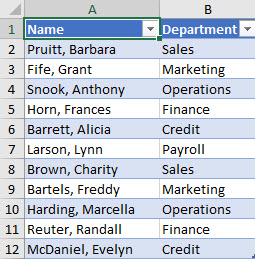
You may want to sort by more than one column or row when you have data that you want to group by the same value in one column or row, and then sort another column or row within that group of equal values. For example, if you have a Department column and an Employee column, you can first sort by Department (to group all the employees in the same department together), and then sort by name (to put the names in alphabetical order within each department). You can sort by up to 64 columns.
Note: For best results, the range of cells that you sort should have column headings.
-
Select any cell in the data range.
-
On the Data tab, in the Sort & Filter group, click Sort.
-
In the Sort dialog box, under Column, in the Sort by box, select the first column that you want to sort.
-
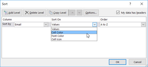
Under Sort On, select the type of sort. Do one of the following:
-
To sort by text, number, or date and time, select Values.
-
To sort by format, select Cell Color, Font Color, or Cell Icon.
-
-
Under Order, select how you want to sort. Do one of the following:
-
For text values, select A to Z or Z to A.
-
For number values, select Smallest to Largest or Largest to Smallest.
-
For date or time values, select Oldest to Newest or Newest to Oldest.
-
To sort based on a custom list, select Custom List.
-
-
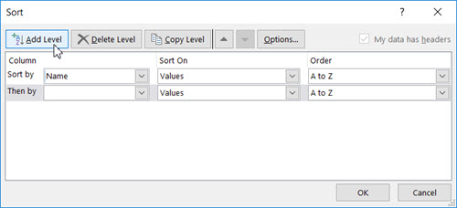
To add another column to sort by, click Add Level, and then repeat steps three through five.
-
To copy a column to sort by, select the entry and then click Copy Level.
-
To delete a column to sort by, select the entry and then click Delete Level.
Note: You must keep at least one entry in the list.
-
To change the order in which the columns are sorted, select an entry and then click the Up or Down arrow next to the Options button to change the order.
Entries higher in the list are sorted before entries lower in the list.

If you have manually or conditionally formatted a range of cells or a table column by cell color or font color, you can also sort by these colors. You can also sort by an icon set that you created with conditional formatting.
-
Select a cell in the column you want to sort.
-
On the Data tab, in the Sort & Filter group, click Sort.
-
In the Sort dialog box, under Column, in the Sort by box, select the column that you want to sort.
-
Under Sort On, select Cell Color, Font Color, or Cell Icon.
-
Under Order, click the arrow next to the button and then, depending on the type of format, select a cell color, font color, or cell icon.
-
Next, select how you want to sort. Do one of the following:
-
To move the cell color, font color, or icon to the top or to the left, select On Top for a column sort, and On Left for a row sort.
-
To move the cell color, font color, or icon to the bottom or to the right, select On Bottom for a column sort, and On Right for a row sort.
Note: There is no default cell color, font color, or icon sort order. You must define the order that you want for each sort operation.
-
-
To specify the next cell color, font color, or icon to sort by, click Add Level, and then repeat steps three through five.
Make sure that you select the same column in the Then by box and that you make the same selection under Order.
Keep repeating for each additional cell color, font color, or icon that you want included in the sort.
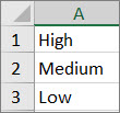
You can use a custom list to sort in a user-defined order. For example, a column might contain values that you want to sort by, such as High, Medium, and Low. How can you sort so that rows containing High appear first, followed by Medium, and then Low? If you were to sort alphabetically, an “A to Z” sort would put High at the top, but Low would come before Medium. And if you sorted “Z to A,” Medium would appear first, with Low in the middle. Regardless of the order, you always want “Medium” in the middle. By creating your own custom list, you can get around this problem.
-
Optionally, create a custom list:
-
In a range of cells, enter the values that you want to sort by, in the order that you want them, from top to bottom as in this example.
-
Select the range that you just entered. Using the preceding example, select cells A1:A3.
-
Go to File > Options > Advanced > General > Edit Custom Lists, then in the Custom Lists dialog box, click Import, and then click OK twice.
Notes:
-
You can create a custom list based only on a value (text, number, and date or time). You cannot create a custom list based on a format (cell color, font color, or icon).
-
The maximum length for a custom list is 255 characters, and the first character must not begin with a number.
-
-
-
Select a cell in the column you want to sort.
-
On the Data tab, in the Sort & Filter group, click Sort.
-
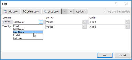
In the Sort dialog box, under Column, in the Sort by or Then by box, select the column that you want to sort by a custom list.
-
Under Order, select Custom List.
-
In the Custom Lists dialog box, select the list that you want. Using the custom list that you created in the preceding example, click High, Medium, Low.
-
Click OK.
-
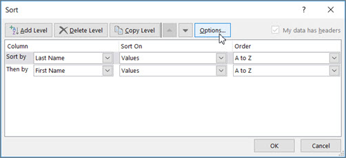
On the Data tab, in the Sort & Filter group, click Sort.
-
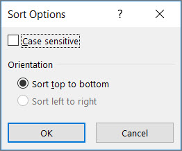
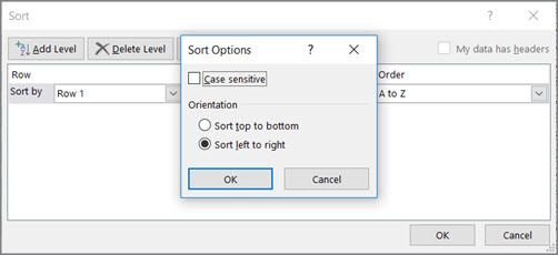
In the Sort dialog box, click Options.
-
In the Sort Options dialog box, select Case sensitive.
-
Click OK twice.
It’s most common to sort from top to bottom, but you can also sort from left to right.
Note: Tables don’t support left to right sorting. To do so, first convert the table to a range by selecting any cell in the table, and then clicking Table Tools > Convert to range.
-
Select any cell within the range you want to sort.
-
On the Data tab, in the Sort & Filter group, click Sort.
-
In the Sort dialog box, click Options.
-
In the Sort Options dialog box, under Orientation, click Sort left to right, and then click OK.
-
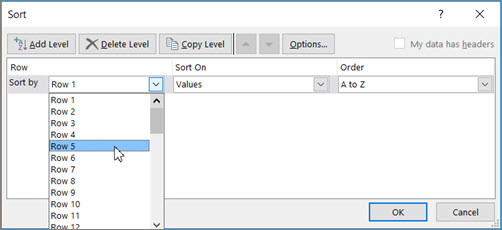
Under Row, in the Sort by box, select the row that you want to sort. This will generally be row 1 if you want to sort by your header row.
Tip: If your header row is text, but you want to order columns by numbers, you can add a new row above your data range and add numbers according to the order you want them.
-
To sort by value, select one of the options from the Order drop-down:
-
For text values, select A to Z or Z to A.
-
For number values, select Smallest to Largest or Largest to Smallest.
-
For date or time values, select Oldest to Newest or Newest to Oldest.
-
-
To sort by cell color, font color, or cell icon, do this:
-
Under Sort On, select Cell Color, Font Color, or Cell Icon.
-
Under Order select a cell color, font color, or cell icon, then select On Left or On Right.
-
Note: When you sort rows that are part of a worksheet outline, Excel sorts the highest-level groups (level 1) so that the detail rows or columns stay together, even if the detail rows or columns are hidden.
To sort by a part of a value in a column, such as a part number code (789-WDG-34), last name (Carol Philips), or first name (Philips, Carol), you first need to split the column into two or more columns so that the value you want to sort by is in its own column. To do this, you can use text functions to separate the parts of the cells or you can use the Convert Text to Columns Wizard. For examples and more information, see Split text into different cells and Split text among columns by using functions.
Warning: It is possible to sort a range within a range, but it is not recommended, because the result disassociates the sorted range from its original data. If you were to sort the following data as shown, the selected employees would be associated with different departments than they were before.
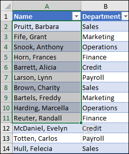
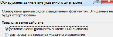
Fortunately, Excel will warn you if it senses you are about to attempt this:

If you did not intend to sort like this, then press the Expand the selection option, otherwise select Continue with the current selection.
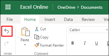
If the results are not what you want, click Undo  .
.
Note: You cannot sort this way in a table.
If you get unexpected results when sorting your data, do the following:
Check to see if the values returned by a formula have changed If the data that you have sorted contains one or more formulas, the return values of those formulas might change when the worksheet is recalculated. In this case, make sure that you reapply the sort to get up-to-date results.
Unhide rows and columns before you sort Hidden columns are not moved when you sort columns, and hidden rows are not moved when you sort rows. Before you sort data, it’s a good idea to unhide the hidden columns and rows.
Check the locale setting Sort orders vary by locale setting. Make sure that you have the proper locale setting in Regional Settings or Regional and Language Options in Control Panel on your computer. For information about changing the locale setting, see the Windows help system.
Enter column headings in only one row If you need multiple line labels, wrap the text within the cell.
Turn on or off the heading row It’s usually best to have a heading row when you sort a column to make it easier to understand the meaning of the data. By default, the value in the heading is not included in the sort operation. Occasionally, you may need to turn the heading on or off so that the value in the heading is or is not included in the sort operation. Do one of the following:
-
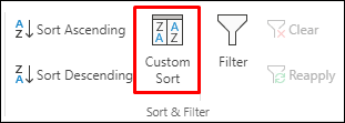
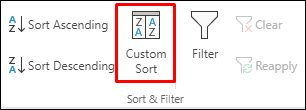
To exclude the first row of data from the sort because it is a column heading, on the Home tab, in the Editing group, click Sort & Filter, click Custom Sort and then select My data has headers.
-
To include the first row of data in the sort because it is not a column heading, on the Home tab, in the Editing group, click Sort & Filter, click Custom Sort, and then clear My data has headers.
If your data is formatted as an Excel table, then you can quickly sort and filter it with the filter buttons in the header row.
-
If your data isn’t already in a table, then format it as a table. This will automatically add a filter button at the top of each table column.
-
Click the filter button at the top of the column you want to sort on, and pick the sort order you want.
-
To undo a sort, use the Undo button on the Home tab.
-
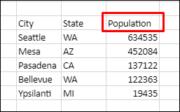
Pick a cell to sort on:
-
If your data has a header row, pick the one you want to sort on, such as Population.
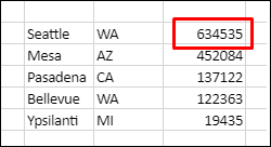
-
If your data doesn’t have a header row, pick the topmost value you want to sort on, such as 634535.
-
-
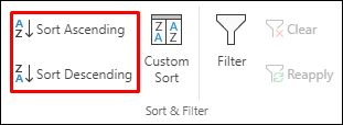
On the Data tab, pick one of the sort methods:
-
Sort Ascending to sort A to Z, smallest to largest, or earliest to latest date.
-
Sort Descending to sort Z to A, largest to smallest, or latest to earliest date.
-
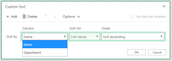
Let’s say you have a table with a Department column and an Employee column. You can first sort by Department to group all the employees in the same department together, and then sort by name to put the names in alphabetical order within each department.
Select any cell within your data range.
-
On the Data tab, in the Sort & Filter group, click Custom Sort.
-
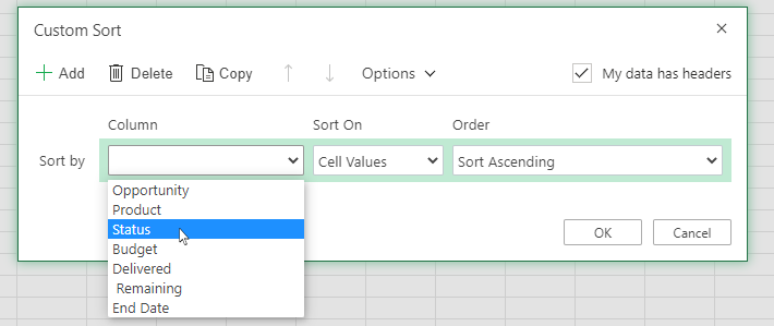
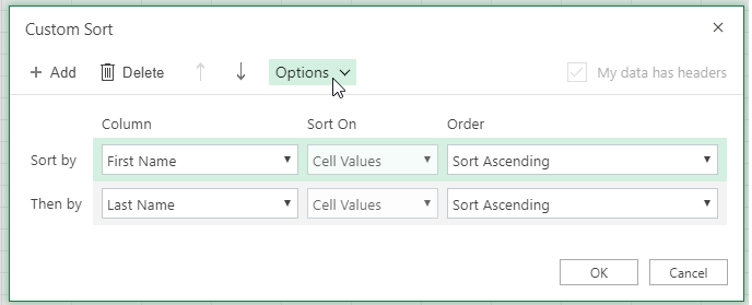
In the Custom Sort dialog box, under Column, in the Sort by box, select the first column that you want to sort.
Note: The Sort On menu is disabled because it’s not yet supported. For now, you can change it in the Excel desktop app.
-
Under Order, select how you want to sort:
-
Sort Ascending to sort A to Z, smallest to largest, or earliest to latest date.
-
Sort Descending to sort Z to A, largest to smallest, or latest to earliest date.
-
-
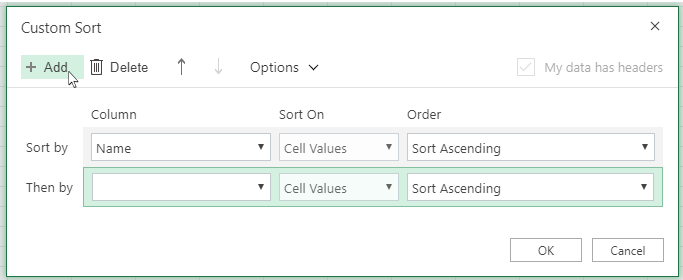
To add another column to sort by, click Add and then repeat steps five and six.
-
To change the order in which the columns are sorted, select an entry and then click the Up or Down arrow next to the Options button.
If you have manually or conditionally formatted a range of cells or a table column by cell color or font color, you can also sort by these colors. You can also sort by an icon set that you created with conditional formatting.
-
Select a cell in the column you want to sort
-
On the Data tab, in the Sort & Filter group, select Custom Sort.
-
In the Custom Sort dialog box under Columns, select the column that you want to sort.
-
Under Sort On, select Cell Color, Font Color or Conditional Formatting Icon.
-
Under Order, select the order you want (what you see depends on the type of format you have). Then select a cell color, font color, or cell icon.
-
Next, you’ll choose how you want to sort by moving the cell color, font color, or icon:
Note: There is no default cell color, font color, or icon sort order. You must define the order that you want for each sort operation.
-
To move to the top or to the left: Select On Top for a column sort, and On Left for a row sort.
-
To move to the bottom or to the right: Select On Bottom for a column sort, and On Right for a row sort.
-
-
To specify the next cell color, font color, or icon to sort by, select Add Level, and then repeat steps 1- 5.
-
Make sure that you the column in the Then by box and the selection under Order are the same.
-
Repeat for each additional cell color, font color, or icon that you want included in the sort.
-
On the Data tab, in the Sort & Filter group, click Custom Sort.
-
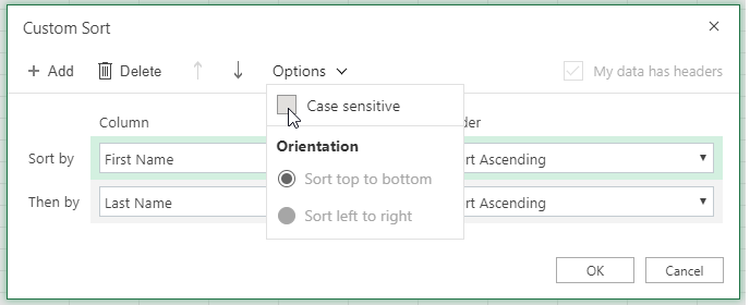
In the Custom Sort dialog box, click Options.
-
In the Options menu, select Case sensitive.
-
Click OK.
It’s most common to sort from top to bottom, but you can also sort from left to right.
Note: Tables don’t support left to right sorting. To do so, first convert the table to a range by selecting any cell in the table, and then clicking Table Tools > Convert to range.
-
Select any cell within the range you want to sort.
-
On the Data tab, in the Sort & Filter group, select Custom Sort.
-
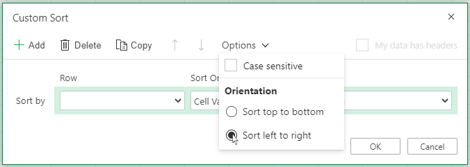
In the Custom Sort dialog box, click Options.
-
Under Orientation, click Sort left to right
-
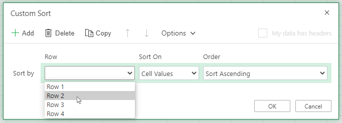
Under Row, in the ‘Sort by’ drop down, select the row that you want to sort. This will generally be row 1 if you want to sort by your header row.
-
To sort by value, select one of the options from the Order drop-down:
-
Sort Ascending to sort A to Z, smallest to largest, or earliest to latest date.
-
Sort Descending to sort Z to A, largest to smallest, or latest to earliest date
-
Need more help?
You can always ask an expert in the Excel Tech Community or get support in the Answers community.
See also
Use the SORT and SORTBY functions to automatically sort your data.
Excel for Microsoft 365 Excel 2021 Excel 2019 Excel 2016 Excel 2013 Excel 2010 More…Less
When sorting information in a worksheet, you can rearrange the data to find values quickly. You can sort a range or table of data on one or more columns of data. For example, you can sort employees —first by department, and then by last name.
How to sort in Excel?
|
|
Select the data to sort Select a range of tabular data, such as A1:L5 (multiple rows and columns) or C1:C80 (a single column). The range can include the first row of headings that identify each column.
|

|
|
Sort quickly and easily
|

|
|
Sort by specifying criteria Use this technique to choose the column you want to sort, together with other criteria such as font or cell colors.
|

Need more help?
![]()
Download Article
![]()
Download Article
Excel is great for tables of data, but how can you manipulate and organize it so that it meets your needs? The Sort tool allows you to quickly sort columns by a variety of formats, or create your own custom sort for multiple columns and types of data. Use the Sort function to logically organize your data and make it easier to understand and use.
-
1
Select your data. You can either click and drag to select the column that you want to sort, or you can click one of the cells in the column to make it active and let Excel select the data automatically.
- All of your data in the column will need to be formatted in the same way in order to sort (i.e. text, numbers, dates).
-
2
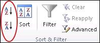
Find the Sort buttons. These can be found in the Data tab in the «Sort & Filter» section. To do quick sorts, you will be using the «AZ↓» and «AZ↑» buttons.
Advertisement
-
3
Sort your column by clicking the appropriate button. If you are sorting numbers, you can sort from lowest to highest («AZ↓») or highest to lowest («AZ↑»). If you are sorting text, you can sort in ascending alphanumeric order («AZ↓») or descending alphanumeric order («AZ↑»). If you are sorting dates or times, you can sort from earlier to later («AZ↓») or later to earlier («AZ↑»).
- If there is another column of data next to the one you are sorting, you will be asked if you want to include that data in the sort. The sort will still be the column you originally selected, but associated columns of data will be sorted along with it.
-
4
Troubleshoot a column that won’t sort. If you are running into errors when you try to sort, the most likely culprit is formatting problems with the data.
- If you are sorting numbers, make sure that all of the cells are formatted as numbers and not text. Numbers can be accidentally imported as text from certain accounting programs.
- If you are sorting text, errors can arise from leading spaces or bad formatting.
- If you are sorting dates or times, troubles usually stem from the formatting of your data. In order for Excel to sort successfully by date, you need to ensure that all of the data is stored as a date.


Advertisement
-
1
Select your data. Let’s say you have a spreadsheet with a list of customer names as well as the city that they are located in. To make your life easier, you want to sort first alphabetically by city, and then sort each customer alphabetically within each city. Creating a custom sort can do just that.
-
2
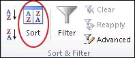
Click the Sort button. This can be found in the «Sort & Filter» section of the Data tab. The Sort window will open, allowing you to create a custom sort with multiple criteria.
- If your columns have headers in the first cell, such as «City» and «Name», make sure to check the «My data has headers» box in the upper-left corner of the sort window.
-
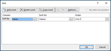
3
Create your first rule. Click the «Sort by» menu to choose the column that you want. In this example, you would first be sorting by city, so select the appropriate column from the menu.
- Keep «Sort on» set to «Values».
- Set the order to either «A to Z» or «Z to A» depending on how you want to sort.
-
4
Create your second rule. Click the «Add Level» button. This will add a rule underneath the first one. Select the second column (The Name column in our example) and then select the sort order (for ease of reading, choose the same order as your first rule).
-
5
Click OK. Your list will be sorted according to your rules. You should see the cities listed alphabetically, and then the customer names sorted alphabetically within each city.
- This example is a simple one and only includes two columns. You can, however, make your sort as complex as you would like, and include many columns.[1]
- This example is a simple one and only includes two columns. You can, however, make your sort as complex as you would like, and include many columns.[1]


Advertisement
-
1
Select your data. You can either click and drag to select the column that you want to sort, or you can click one of the cells in the column to make it active and let Excel select the data automatically.
-
2
Click the Sort button. The Sort button can be found in the Data tab in the «Sort & Filter» section. This will open the Sort window. If you have another column of data next to the one you are sorting, you will be asked if you want to include that data in the sort.
-
3
Select «Cell Color» or «Font Color» in the «Sort On» menu. This will allow you to choose the first color you want to sort by.
-
4
Select which color you want to sort first. In the «Order» column, you can use the drop down menu to choose which color you want to put first or last in the sort. You can only choose colors that are present in the column.
- There is no default order for color sorting. You will need to define the order yourself.
-
5
Add another color. You will need to add another rule for each color in the column you are sorting. Click the «Add Level» to add another rule to the sort. Choose the next color that you want to sort by, and then the order that you want to sort.
- Make sure that each order is the same for each rule. For example, if you are sorting from top to bottom, make sure the «Order» section for each rule says «On Top».
-
6
Click OK. Each rule will be applied one by one, and the column will be sorted by the colors you defined.


Advertisement
Add New Question
-
Question
How can the sort function on Microsoft Word help me?

Let’s say you are a teacher and you have a database of students with their assignment grades. By sorting on assignment type and grade received, you can find the students who need more help. In other words, sorting allows one to focus attention where it is most needed.
-
Question
I tried to sort by color, but the only thing in the Sort On dropdown is «no cell color». Why do I not have any colors to choose from?
You have to format your data’s cells with colors first in order to sort by color.
-
Question
How do I store results of a sort into a new table while retaining the original table?
Copy the table (and show results of your sort) into a new page.
Ask a Question
200 characters left
Include your email address to get a message when this question is answered.
Submit
Advertisement
wikiHow Video: How to Sort a List in Microsoft Excel
-
Try sorting data in different ways; these new perspectives can illuminate different aspects of the information.
-
If your spreadsheet has totals, averages or other summary information below the information you need to sort, be careful not to sort those as well.
Thanks for submitting a tip for review!
Advertisement
-
Be extremely careful to select all of the columns you need when sorting.
Advertisement
References
About This Article
Article SummaryX
To sort your data alphabetically or numerically, start by highlighting the cells you want to sort. Then, click the «Data» tab at the top of Excel. In the «Sort & Filter» panel in the toolbar, click the AZ with a down-arrow to sort in alphabetical or numerical order, starting with the smallest values first, or AZ with an up-arrow to reverse that sorting method, or starting with the largest values first. You can also sort by font or cell color. With your data selected, click the Data tab, and then click «Sort» on the «Sort & Filter» panel. If your data has headers, check the box near the top-right corner. Select a column, and then choose how to sort it, such as by cell or font Color. Click the «Order» menu to choose a color to sort first, and select «On Top» from the drop-down menu. To add the next color in the sequence, click «Add Level,» and select the same column and sorting method. Choose the color that should appear next and select «On Top» again. Keep adding rules for the column until you’ve placed all colors in order, and then click «OK» to sort. Just like adding rules to sort by color, you can add rules to sort columns by multiple criteria, such as both alphabetically and by cell color. In the Sort window, select a column, and then enter the sorting method and criteria. Click «Add Level» to add another rule, pick the same column, and then choose a different sorting method. Click «OK» when you’re finished to save and sort.
Did this summary help you?
Thanks to all authors for creating a page that has been read 231,999 times.
Is this article up to date?
Сортировка данных в Excel – инструмент для представления информации в удобном для пользователя виде.
Числовые значения можно отсортировать по возрастанию и убыванию, текстовые – по алфавиту и в обратном порядке. Доступны варианты – по цвету и шрифту, в произвольном порядке, по нескольким условиям. Сортируются столбцы и строки.
Порядок сортировки в Excel
Существует два способа открыть меню сортировки:
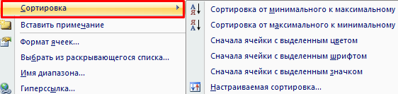
- Щелкнуть правой кнопкой мыши по таблице. Выбрать «Сортировку» и способ.
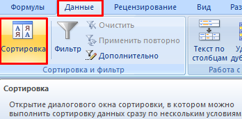
- Открыть вкладку «Данные» — диалоговое окно «Сортировка».
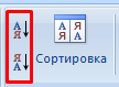
Часто используемые методы сортировки представлены одной кнопкой на панели задач:
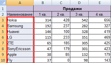
Сортировка таблицы по отдельному столбцу:
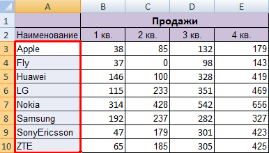
- Чтобы программа правильно выполнила задачу, выделяем нужный столбец в диапазоне данных.
- Далее действуем в зависимости от поставленной задачи. Если нужно выполнить простую сортировку по возрастанию/убыванию (алфавиту или обратно), то достаточно нажать соответствующую кнопку на панели задач. Когда диапазон содержит более одного столбца, то Excel открывает диалоговое окно вида:
Чтобы сохранилось соответствие значений в строках, выбираем действие «автоматически расширить выделенный диапазон». В противном случае отсортируется только выделенный столбец – структура таблицы нарушится.
Если выделить всю таблицу и выполнить сортировку, то отсортируется первый столбец. Данные в строках станут в соответствии с положением значений в первом столбце.
Сортировка по цвету ячейки и по шрифту
Программа Excel предоставляет пользователю богатые возможности форматирования. Следовательно, можно оперировать разными форматами.
Сделаем в учебной таблице столбец «Итог» и «зальем» ячейки со значениями разными оттенками. Выполним сортировку по цвету:
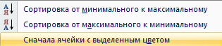
- Выделяем столбец – правая кнопка мыши – «Сортировка».
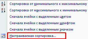
- Из предложенного списка выбираем «Сначала ячейки с выделенным цветом».
- Соглашаемся «автоматически расширить диапазон».
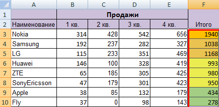
Программа отсортировала ячейки по акцентам. Пользователь может самостоятельно выбрать порядок сортировки цвета. Для этого в списке возможностей инструмента выбираем «Настраиваемую сортировку».
В открывшемся окне вводим необходимые параметры:
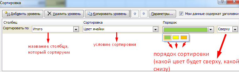
Здесь можно выбрать порядок представления разных по цвету ячеек.
По такому же принципу сортируются данные по шрифту.
Сортировка в Excel по нескольким столбцам
Как задать порядок вторичной сортировки в Excel? Для решения этой задачи нужно задать несколько условий сортировки.
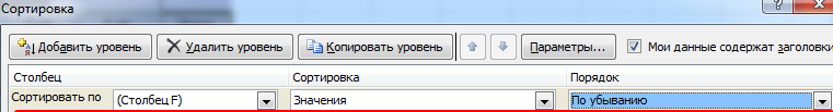
- Открываем меню «Настраиваемая сортировка». Назначаем первый критерий.
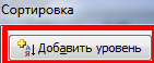
- Нажимаем кнопку «Добавить уровень».
- Появляются окошки для введения данных следующего условия сортировки. Заполняем их.
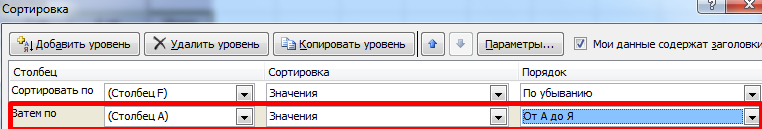
Программа позволяет добавить сразу несколько критериев чтобы выполнить сортировку в особом порядке.
Сортировка строк в Excel
По умолчанию сортируются данные по столбцам. Как осуществить сортировку по строкам в Excel:
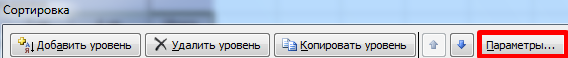
- В диалоговом окне «Настраиваемой сортировки» нажать кнопку «Параметры».
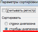
- В открывшемся меню выбрать «Столбцы диапазона».
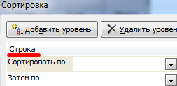
- Нажать ОК. В окне «Сортировки» появятся поля для заполнения условий по строкам.
Таким образом выполняется сортировка таблицы в Excel по нескольким параметрам.
Случайная сортировка в Excel
Встроенные параметры сортировки не позволяют расположить данные в столбце случайным образом. С этой задачей справится функция СЛЧИС.
Например, нужно расположить в случайном порядке набор неких чисел.
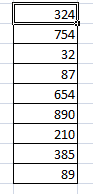
Ставим курсор в соседнюю ячейку (слева-справа, не важно). В строку формул вводим СЛЧИС(). Жмем Enter. Копируем формулу на весь столбец – получаем набор случайных чисел.
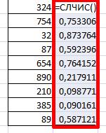
Теперь отсортируем полученный столбец по возрастанию /убыванию – значения в исходном диапазоне автоматически расположатся в случайном порядке.
Динамическая сортировка таблицы в MS Excel
Если применить к таблице стандартную сортировку, то при изменении данных она не будет актуальной. Нужно сделать так, чтобы значения сортировались автоматически. Используем формулы.
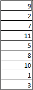
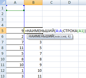
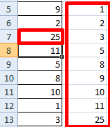
- Есть набор простых чисел, которые нужно отсортировать по возрастанию.
- Ставим курсор в соседнюю ячейку и вводим формулу: =НАИМЕНЬШИЙ(A:A;СТРОКА(A1)). Именно так. В качестве диапазона указываем весь столбец. А в качестве коэффициента – функцию СТРОКА со ссылкой на первую ячейку.
- Изменим в исходном диапазоне цифру 7 на 25 – «сортировка» по возрастанию тоже изменится.
Если необходимо сделать динамическую сортировку по убыванию, используем функцию НАИБОЛЬШИЙ.
Для динамической сортировки текстовых значений понадобятся формулы массива.
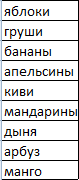
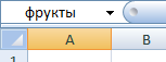
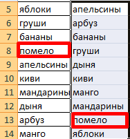
- Исходные данные – перечень неких названий в произвольном порядке. В нашем примере – список фруктов.
- Выделяем столбец и даем ему имя «Фрукты». Для этого в поле имен, что находится возле строки формул вводим нужное нам имя для присвоения его к выделенному диапазону ячеек.
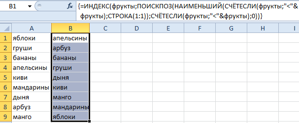
- В соседней ячейке (в примере – в В5) пишем формулу: Так как перед нами формула массива, нажимаем сочетание Ctrl + Shift + Enter. Размножаем формулу на весь столбец.
- Если в исходный столбец будут добавляться строки, то вводим чуть модифицированную формулу: Добавим в диапазон «фрукты» еще одно значение «помело» и проверим:
Скачать формулы сортировки данных в Excel
Впоследствии при добавлении данных в таблицу процесс сортирования будет выполняться автоматически.
When you have large amounts of data, it can be overwhelming if it’s not sorted correctly in your workbook. Learn different methods to sort data in Excel to become more productive and to make your spreadsheets easier to manage.
Instructions in this article apply to Excel 2019, 2016, 2013, 2010; Excel for Microsoft 365, Excel Online, and Excel for Mac.
Select Data to be Sorted
Before data can be sorted, Excel needs to know the exact range that is to be sorted. Excel will select areas of related data as long as the data meets these conditions:
- There are no blank rows or columns in an area of related data.
- Blank rows and columns are between areas of related data.
Excel determines if the data area has field names and excludes the row from the records to be sorted. Allowing Excel to select the range to be sorted can be risky, especially with large amounts of data that are hard to check.
To ensure that the correct data is selected, highlight the range before starting the sort. If the same range will be sorted repeatedly, the best approach is to give it a Name.
Sort Key and Sort Order in Excel
Sorting requires the use of a sort key and a sort order. The sort key is the data in the column or columns you want to sort and is identified by the column heading or field name. In the image below, the possible sort keys are Student ID, Name, Age, Program, and Month Started.
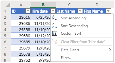
Sort Data Quickly
To do a quick sort, select a single cell in the column containing the sort key. Then choose how you want the data sorted. Here’s how:
- Select a cell in the column containing the sort key.
- Select Home.
- Select Sort & Filter to open the drop-down menu of sort options.
- Choose how you want to sort the data. Select either ascending or descending order.
When using Sort & Filter, the sort order options in the drop-down list change depending upon the type of data in the selected range. For text data, the options are Sort A to Z and Sort Z to A. For numeric data, the options are Sort Smallest to Largest and Sort Largest to Smallest.
Sort Multiple Columns of Data in Excel
In addition to performing a quick sort based on a single column of data, Excel’s custom sort feature allows you to sort on multiple columns by defining multiple sort keys. In multi-column sorts, the sort keys are identified by selecting the column headings in the Sort dialog box.
As with a quick sort, the sort keys are defined by identifying the columns headings or field names, in the table containing the sort key.
Sort on Multiple Columns Example
In the example below, the data in the range A2 to E12 is sorted on two columns of data. The data is first sorted by name and then by age.
To sort multiple columns of data:
- Highlight the range of cells to be sorted. In this example, cells A2 to E12 are selected.
- Select Home.
- Select Sort & Filter to open the drop-down list.
- Select Custom Sort to open the Sort dialog box.
- Place a check next to My data has headers.
- Under the Column heading, select the Sort by down arrow and choose Name from the drop-down list to first sort the data by the Name column.
- Under the Sort On heading, leave the setting as Cell Values. The sort is based on the actual data in the table.
- Under the Order heading, select the down arrow and choose Z to A to sort the Name data in descending order.
- Select Add Level to add a second sort option.
- Under the Column heading, select the Then by down arrow and choose Age to sort records with duplicate names by the Age column.
- Under the Order heading, choose Largest to Smallest from the drop-down list to sort the Age data in descending order.
- Select OK to close the dialog box and sort the data.
As a result of defining a second sort key, shown in the example below, the two records with identical values for the Name field are sorted in descending order using the Age field. This results in the record for the student Wilson J., age 21, being before the record for Wilson P., age 19.
The First Row: Column Headings or Data
The range of data selected for sorting in the example above included the column headings above the first row of data. This row contains data that is different from the data in subsequent rows. Excel determined that the first row contains the column headings and adjusted the available options in the Sort dialog box to include them.
Excel uses formatting to determine whether a row contains column headings. In the example above, the column headings are a different font from the data in the rest of the rows.
If the first row does not contain headings, Excel uses the column letter (such as Column D or Column E) as choices in the Column option of the Sort dialog box.
Excel uses this difference to make a determination on whether the first row is a heading row. If Excel makes a mistake, the Sort dialog box contains a My data has headers checkbox that overrides this automatic selection.
Sort Data by Date or Time in Excel
In addition to sorting text data alphabetically or numbers from largest to smallest, Excel’s sort options include sorting date values. Available sort orders available for dates include:
- Ascending order: Oldest to newest.
- Descending order: Newest to oldest.
Quick Sort vs. Sort Dialog Box
Dates and times that are formatted as number data, such as Date Borrowed in the example above, use the quick sort method to sort on a single column. For sorts involving multiple columns of dates or times, use the Sort dialog box in the same way as sorting multiple columns of number or text data.
Sort by Date Example
To perform a quick sort by date in ascending order, from oldest to newest:
- Highlight the range of cells to be sorted. To follow the example above, highlight cells G2 to K7.
- Select Home.
- Select Sort & Filter to open the drop-down list.
- Select Custom Sort to open the Sort dialog box.
- Under the Column heading, select the Sort by down arrow and choose Borrowed to first sort the data by the borrowed date.
- Under the Sort On heading, choose Cell Values. The sort is based on the actual data in the table.
- Under the Sort Order heading, choose Oldest to Newest from the drop-down list.
- Select OK in the dialog box to close the dialog box and sort the data.
If the results of sorting by date do not turn out as expected, the data in the column containing the sort key might contain dates or times stored as text data rather than as numbers (dates and times are just formatted number data).
Mixed Data and Quick Sorts
When using the quick sort method, if records containing text and number data are mixed together, Excel sorts the number and text data separately by placing the records with text data at the bottom of the sorted list.
Excel might also include the column headings in the sort results, interpreting them as just another row of text data rather than as the field names for the data table.
Possible Sort Warning
If the Sort dialog box is used, even for sorts on one column, Excel may display a message warning you that it has encountered data stored as text and gives you the choice to:
- Sort anything that looks like a number as a number.
- Sort numbers and numbers stored as text separately.
If you choose the first option, Excel attempts to place the text data in the correct location of the sort results. Choose the second option and Excel places the records containing text data at the bottom of the sort results, just as it does with quick sorts.
Sort Data by Days of the Week or by Months in Excel
You can also sort data by days of the week or by months of the year using the same built-in custom list that Excel uses to add days or months to a worksheet using the fill handle. These lists allow sorting by days or months chronologically rather than in alphabetical order.
As with other sort options, sorting values by a custom list can be displayed in ascending (Sunday to Saturday or January to December) or descending order (Saturday to Sunday or December to January).
In the image above, the following steps were followed to sort the data sample in the range A2 to E12 by months of the year:
- Highlight the range of cells to be sorted.
- Select Home.
- Select Sort & Filter to open the drop-down list.
- Select Custom Sort to open the Sort dialog box.
- Under the Column heading, choose Month Start from the drop-down list to sort the data by the months of the year.
- Under the Sort On heading, select Cell Values. The sort is based on the actual data in the table.
- Under the Order heading, select the down arrow next to the default A to Z option to open the drop-down menu.
- Choose Custom List to open the Custom Lists dialog box.
- In the left-hand window of the dialog box, select January, February, March, April.
- Select OK to confirm the selection and return to the Sort the dialog box.
- The chosen list (January, February, March, April) displays under the Order heading.
- Select OK to close the dialog box and sort the data by months of the year.
By default, custom lists are displayed only in ascending order in the Custom Lists dialog box. To sort data in descending order using a custom list after having selected the desired list so that it is displayed under the Order heading in the Sort dialog box:
- Select the down arrow next to the displayed list, such as January, February, March, April to open the drop-down menu.
- In the menu, select the custom list option that is displayed in descending order, such as December, November, October, September.
- Click OK to sort the data in descending order using the custom list.
Sort by Rows to Reorder Columns in Excel
As shown with the previous sort options, data is normally sorted using column headings or field names. The result is the reordering of entire rows or records of data. A less known, and therefore, less used sort option in Excel is to sort by row, which has the effect of rearranging the order of columns left to right in a worksheet.
One reason for sorting by row is to match the column order between different tables of data. With the columns in the same left to right order, it is easier to compare records or to copy and move data between the tables.
Customize the Column Order
Very seldom, however, is getting the columns in the correct order a straightforward task due to the limitations of the ascending and descending sort order options for values. Usually, it is necessary to use a custom sort order, and Excel includes options for sorting by cell or font color or by conditional formatting icons.
The easiest way of telling Excel the order of columns is to add a row above or below the data table containing numbers that indicate the order of columns from left to right. Sorting by rows then becomes a simple matter of sorting the columns smallest to largest by the row containing the numbers.
Once the sort is done, the added row of numbers can easily be deleted.
Sort by Rows Example
In the data sample used for this series on Excel sort options, the Student ID column has always been first on the left, followed by Name and then Age.
In this instance, as shown in the image above, numbers have been added to the columns to prepare the worksheet to reorder the columns so that the Program column is first on the left followed by Month Start, Name, Age, and Student ID.
Here’s how to change the column order:
- Insert a blank row above the row containing the field names.
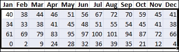
- In this new row, enter the following numbers left to right starting in column A: 5, 3, 4, 1, 2.
- Highlight the range to be sorted. In this example, highlight A2 to E13.
- Select Home.
- Select Sort & Filter to open the drop-down list.
- Select Custom Sort to open the Sort dialog box.
- Select Options to open the Sort Options dialog box.
- In the Orientation section, select Sort left to right to sort the order of columns left to right in the worksheet.
- Select OK to close the Sort Options dialog box.
- With the change in Orientation, the Column heading in the Sort dialog box changes to Row.
- Select the Sort by down arrow and choose Row 2. This is the row containing the custom numbers.
- Under the Sort On heading, choose Cell Values.
- Under the Order heading, choose Smallest to Largest from the drop-down list to sort the numbers in row 2 in ascending order.
- Select OK to close the dialog box and sort the columns left to right by the numbers in row 2.
- The order of columns begins with Program followed by Month Start, Name, Age, and Student ID.
Use Excel’s Custom Sort Options to Reorder Columns
While custom sorts are available in the Sort dialog box in Excel, these options are not easy to use when it comes to reordering columns in a worksheet. Options for creating a custom sort order available in the Sort dialog box are to sort the data by cell color, font color, and icon.
Unless each column has already had unique formatting applied, such as different font or cell colors, that formatting needs to be added to individual cells in the same row for each column to be reordered.
For example, to use font color to reorder the columns:
- Select each field name and change the font color for each. For example, change Program to red, Month Start to green, Name to blue, Age to orange, and Student ID to purple.
- In the Sort dialog box, select Sort by and choose Row 2.
- Under the Sort on heading, choose Font Color.
- Under the Order heading, manually set the order of field names colors to match the desired column order.
- After sorting, reset the font color for each field name.