How do i link cells on excel - Word и Excel - помощь в работе с программами

Excel for Microsoft 365 Excel for the web Excel 2021 Excel 2019 Excel 2016 Excel 2013 Excel 2010 Excel 2007 More…Less

You can refer to the contents of cells in another workbook by creating an external reference formula. An external reference (also called a link) is a reference to a cell or range on a worksheet in another Excel workbook, or a reference to a defined name in another workbook.

Open the workbook that will contain the external reference (the destination workbook) and the workbook that contains the data that you want to link to (the source workbook).
Select the cell or cells where you want to create the external reference.
Type = (equal sign).

If you want to use a function, such as SUM, then type the function name followed by an opening parenthesis. For example, =SUM(.
Switch to the source workbook, and then click the worksheet that contains the cells that you want to link.
Select the cell or cells that you want to link to and press Enter.

Note: If you select multiple cells, like =[SourceWorkbook.xlsx]Sheet1!$A$1:$A$10, and have a current version of Microsoft 365, then you can simply press ENTER to confirm the formula as a dynamic array formula. Otherwise, the formula must be entered as a legacy array formula by pressing CTRL+SHIFT+ENTER. For more information on array formulas, see Guidelines and examples of array formulas.
Excel will return you to the destination workbook and display the values from the source workbook.
Note that Excel will return the link with absolute references, so if you want to copy the formula to other cells, you’ll need to remove the dollar ($) signs:

=[SourceWorkbook.xlsx]Sheet1!$A$1

If you close the source workbook, Excel will automatically append the file path to the formula:

=’C:Reports[SourceWorkbook.xlsx]Sheet1′!$A$1

Open the workbook that will contain the external reference (the destination workbook) and the workbook that contains the data that you want to link to (the source workbook).
Select the cell or cells where you want to create the external reference.
Type = (equal sign).
Switch to the source workbook, and then click the worksheet that contains the cells that you want to link.
Press F3, select the name that you want to link to and press Enter.

Note: If the named range references multiple cells, and you have a current version of Microsoft 365, then you can simply press ENTER to confirm the formula as a dynamic array formula. Otherwise, the formula must be entered as a legacy array formula by pressing CTRL+SHIFT+ENTER. For more information on array formulas, see Guidelines and examples of array formulas.
Excel will return you to the destination workbook and display the values from the named range in the source workbook.

Open the destination workbook and the source workbook.
In the destination workbook, Go to Formulas > Defined Names > Define Name.
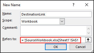
In the New Name dialog box, in the Name box, type a name for the range.
In the Refers to box, delete the contents, and then keep the cursor in the box.

If you want the name to use a function, enter the function name, and then position the cursor where you want the external reference. For example, type =SUM(), and then position the cursor between the parentheses.
Switch to the source workbook, and then click the worksheet that contains the cells that you want to link.
Select the cell or range of cells that you want to link, and click OK.

External references are especially useful when it’s not practical to keep large worksheet models together in the same workbook.

Merge data from several workbooks You can link workbooks from several users or departments and then integrate the pertinent data into a summary workbook. That way, when the source workbooks are changed, you won’t have to manually change the summary workbook.
Create different views of your data You can enter all of your data into one or more source workbooks, and then create a report workbook that contains external references to only the pertinent data.
Streamline large, complex models By breaking down a complicated model into a series of interdependent workbooks, you can work on the model without opening all of its related sheets. Smaller workbooks are easier to change, don’t require as much memory, and are faster to open, save, and calculate.

Formulas with external references to other workbooks are displayed in two ways, depending on whether the source workbook — the one that supplies data to a formula — is open or closed.

When the source is open, the external reference includes the workbook name in square brackets ([ ]), followed by the worksheet name, an exclamation point (!), and the cells that the formula depends on. For example, the following formula adds the cells C10:C25 from the workbook named Budget.xls.

External reference
=SUM([Budget.xlsx]Annual!C10:C25)

When the source is not open, the external reference includes the entire path.

External reference
=SUM(‘C:Reports[Budget.xlsx]Annual’!C10:C25)

Note: If the name of the other worksheet or workbook contains spaces or non-alphabetical characters, you must enclose the name (or the path) within single quotation marks as in the example above. Excel will automatically add these for you when you select the source range.

Formulas that link to a defined name in another workbook use the workbook name followed by an exclamation point (!) and the name. For example, the following formula adds the cells in the range named Sales from the workbook named Budget.xlsx.

External reference
=SUM(Budget.xlsx!Sales)

Select the cell or cells where you want to create the external reference.
Type = (equal sign).

If you want to use a function, such as SUM, then type the function name followed by an opening parenthesis. For example, =SUM(.
Switch to the worksheet that contains the cells that you want to link to.
Select the cell or cells that you want to link to and press Enter.

Note: If you select multiple cells (=Sheet1!A1:A10), and have a current version of Microsoft 365, then you can simply press ENTER to confirm the formula as a dynamic array formula. Otherwise, the formula must be entered as a legacy array formula by pressing CTRL+SHIFT+ENTER. For more information on array formulas, see Guidelines and examples of array formulas.
Excel will return to the original worksheet and display the values from the source worksheet.

Create an external reference between cells in different workbooks

Open the workbook that will contain the external reference (the destination workbook, also called the formula workbook) and the workbook that contains the data that you want to link to (the source workbook, also called the data workbook).
In the source workbook, select the cell or cells you want to link.
Press Ctrl+C or go to Home > Clipboard > Copy.
Switch to the destination workbook, and then click the worksheet where you want the linked data to be placed.
Select the cell where you want to place the linked data, then go to Home > Clipboard > Paste > Paste Link.
Excel will return the data you copied from the source workbook. If you change it, it will automatically change in the destination workbook when you refresh your browser window.
To use the link in a formula, type = in front of the link, choose a function, type (, and then type ) after the link.

Create a link to a worksheet in the same workbook

Select the cell or cells where you want to create the external reference.
Type = (equal sign).

If you want to use a function, such as SUM, then type the function name followed by an opening parenthesis. For example, =SUM(.
Switch to the worksheet that contains the cells that you want to link to.
Select the cell or cells that you want to link to and press Enter.
Excel will return to the original worksheet and display the values from the source worksheet.

Need more help?

You can always ask an expert in the Excel Tech Community or get support in the Answers community.

HYPERLINK function

This article describes the formula syntax and usage of the HYPERLINK function in Microsoft Excel.

Description

The HYPERLINK function creates a shortcut that jumps to another location in the current workbook, or opens a document stored on a network server, an intranet, or the Internet. When you click a cell that contains a HYPERLINK function, Excel jumps to the location listed, or opens the document you specified.

Syntax

The HYPERLINK function syntax has the following arguments:

Link_location Required. The path and file name to the document to be opened. Link_location can refer to a place in a document — such as a specific cell or named range in an Excel worksheet or workbook, or to a bookmark in a Microsoft Word document. The path can be to a file that is stored on a hard disk drive. The path can also be a universal naming convention (UNC) path on a server (in Microsoft Excel for Windows) or a Uniform Resource Locator (URL) path on the Internet or an intranet.

Note Excel for the web the HYPERLINK function is valid for web addresses (URLs) only. Link_location can be a text string enclosed in quotation marks or a reference to a cell that contains the link as a text string.

If the jump specified in link_location does not exist or cannot be navigated, an error appears when you click the cell.

Friendly_name Optional. The jump text or numeric value that is displayed in the cell. Friendly_name is displayed in blue and is underlined. If friendly_name is omitted, the cell displays the link_location as the jump text.

Friendly_name can be a value, a text string, a name, or a cell that contains the jump text or value.

If friendly_name returns an error value (for example, #VALUE!), the cell displays the error instead of the jump text.

In the Excel desktop application, to select a cell that contains a hyperlink without jumping to the hyperlink destination, click the cell and hold the mouse button until the pointer becomes a cross , then release the mouse button. In Excel for the web, select a cell by clicking it when the pointer is an arrow; jump to the hyperlink destination by clicking when the pointer is a pointing hand.

Examples

=HYPERLINK(«http://example.microsoft.com/report/budget report.xlsx», «Click for report»)

Opens a workbook saved at http://example.microsoft.com/report. The cell displays «Click for report» as its jump text.

=HYPERLINK(«[http://example.microsoft.com/report/budget report.xlsx]Annual!F10», D1)

Creates a hyperlink to cell F10 on the Annual worksheet in the workbook saved at http://example.microsoft.com/report. The cell on the worksheet that contains the hyperlink displays the contents of cell D1 as its jump text.

=HYPERLINK(«[http://example.microsoft.com/report/budget report.xlsx]’First Quarter’!DeptTotal», «Click to see First Quarter Department Total»)

Creates a hyperlink to the range named DeptTotal on the First Quarter worksheet in the workbook saved at http://example.microsoft.com/report. The cell on the worksheet that contains the hyperlink displays «Click to see First Quarter Department Total» as its jump text.

=HYPERLINK(«http://example.microsoft.com/Annual Report.docx]QrtlyProfits», «Quarterly Profit Report»)

To create a hyperlink to a specific location in a Word file, you use a bookmark to define the location you want to jump to in the file. This example creates a hyperlink to the bookmark QrtlyProfits in the file Annual Report.doc saved at http://example.microsoft.com.

Displays the contents of cell D5 as the jump text in the cell and opens the workbook saved on the FINANCE server in the Statements share. This example uses a UNC path.

Opens the workbook 1stqtr.xlsx that is stored in the Finance directory on drive D, and displays the numeric value that is stored in cell H10.

Creates a hyperlink to the Totals area in another (external) workbook, Mybook.xlsx.

=HYPERLINK(«[Book1.xlsx]Sheet1!A10″,»Go to Sheet1 > A10»)

To jump to a different location in the current worksheet, include both the workbook name, and worksheet name like this, where Sheet1 is the current worksheet.

=HYPERLINK(«[Book1.xlsx]January!A10″,»Go to January > A10»)

To jump to a different location in the current worksheet, include both the workbook name, and worksheet name like this, where January is another worksheet in the workbook.

=HYPERLINK(CELL(«address»,January!A1),»Go to January > A1″)

To jump to a different location in the current worksheet without using the fully qualified worksheet reference ([Book1.xlsx]), you can use this, where CELL(«address») returns the current workbook name.

To quickly update all formulas in a worksheet that use a HYPERLINK function with the same arguments, you can place the link target in another cell on the same or another worksheet, and then use an absolute reference to that cell as the link_location in the HYPERLINK formulas. Changes that you make to the link target are immediately reflected in the HYPERLINK formulas.

Источник

Create an external reference (link) to a cell range in another workbook

Open the workbook that will contain the external reference (the destination workbook) and the workbook that contains the data that you want to link to (the source workbook).

Select the cell or cells where you want to create the external reference.

Type = (equal sign).

If you want to use a function, such as SUM, then type the function name followed by an opening parenthesis. For example, =SUM(.

Switch to the source workbook, and then click the worksheet that contains the cells that you want to link.

Select the cell or cells that you want to link to and press Enter.

Note: If you select multiple cells, like =[SourceWorkbook.xlsx]Sheet1!$A$1:$A$10, and have a current version of Microsoft 365, then you can simply press ENTER to confirm the formula as a dynamic array formula. Otherwise, the formula must be entered as a legacy array formula by pressing CTRL+SHIFT+ENTER. For more information on array formulas, see Guidelines and examples of array formulas.

Excel will return you to the destination workbook and display the values from the source workbook.

Note that Excel will return the link with absolute references, so if you want to copy the formula to other cells, you’ll need to remove the dollar ($) signs:

=[SourceWorkbook.xlsx]Sheet1! $A $1

If you close the source workbook, Excel will automatically append the file path to the formula:

Open the workbook that will contain the external reference (the destination workbook) and the workbook that contains the data that you want to link to (the source workbook).

Select the cell or cells where you want to create the external reference.

Type = (equal sign).

Switch to the source workbook, and then click the worksheet that contains the cells that you want to link.

Press F3, select the name that you want to link to and press Enter.

Note: If the named range references multiple cells, and you have a current version of Microsoft 365, then you can simply press ENTER to confirm the formula as a dynamic array formula. Otherwise, the formula must be entered as a legacy array formula by pressing CTRL+SHIFT+ENTER. For more information on array formulas, see Guidelines and examples of array formulas.

Excel will return you to the destination workbook and display the values from the named range in the source workbook.

Open the destination workbook and the source workbook.

In the destination workbook, Go to Formulas > Defined Names > Define Name.

In the New Name dialog box, in the Name box, type a name for the range.

In the Refers to box, delete the contents, and then keep the cursor in the box.

If you want the name to use a function, enter the function name, and then position the cursor where you want the external reference. For example, type =SUM(), and then position the cursor between the parentheses.

Switch to the source workbook, and then click the worksheet that contains the cells that you want to link.

Select the cell or range of cells that you want to link, and click OK.

Defined Names > Define Name > New Name.» loading=»lazy»>

External references are especially useful when it’s not practical to keep large worksheet models together in the same workbook.

Merge data from several workbooks You can link workbooks from several users or departments and then integrate the pertinent data into a summary workbook. That way, when the source workbooks are changed, you won’t have to manually change the summary workbook.

Create different views of your data You can enter all of your data into one or more source workbooks, and then create a report workbook that contains external references to only the pertinent data.

Streamline large, complex models By breaking down a complicated model into a series of interdependent workbooks, you can work on the model without opening all of its related sheets. Smaller workbooks are easier to change, don’t require as much memory, and are faster to open, save, and calculate.

Formulas with external references to other workbooks are displayed in two ways, depending on whether the source workbook — the one that supplies data to a formula — is open or closed.

When the source is open, the external reference includes the workbook name in square brackets ( [ ]), followed by the worksheet name, an exclamation point ( !), and the cells that the formula depends on. For example, the following formula adds the cells C10:C25 from the workbook named Budget.xls.

When the source is not open, the external reference includes the entire path.

Note: If the name of the other worksheet or workbook contains spaces or non-alphabetical characters, you must enclose the name (or the path) within single quotation marks as in the example above. Excel will automatically add these for you when you select the source range.

Select the cell or cells where you want to create the external reference.

Type = (equal sign).

If you want to use a function, such as SUM, then type the function name followed by an opening parenthesis. For example, =SUM(.

Switch to the worksheet that contains the cells that you want to link to.

Select the cell or cells that you want to link to and press Enter.

Note: If you select multiple cells (=Sheet1!A1:A10), and have a current version of Microsoft 365, then you can simply press ENTER to confirm the formula as a dynamic array formula. Otherwise, the formula must be entered as a legacy array formula by pressing CTRL+SHIFT+ENTER. For more information on array formulas, see Guidelines and examples of array formulas.

Excel will return to the original worksheet and display the values from the source worksheet.

Create an external reference between cells in different workbooks

Open the workbook that will contain the external reference (the destination workbook, also called the formula workbook) and the workbook that contains the data that you want to link to (the source workbook, also called the data workbook).

In the source workbook, select the cell or cells you want to link.

Press Ctrl+C or go to Home > Clipboard > Copy.

Switch to the destination workbook, and then click the worksheet where you want the linked data to be placed.

Select the cell where you want to place the linked data, then go to Home > Clipboard > Paste > Paste Link.

Excel will return the data you copied from the source workbook. If you change it, it will automatically change in the destination workbook when you refresh your browser window.

To use the link in a formula, type = in front of the link, choose a function, type (, and then type ) after the link.

Create a link to a worksheet in the same workbook

Select the cell or cells where you want to create the external reference.

Type = (equal sign).

If you want to use a function, such as SUM, then type the function name followed by an opening parenthesis. For example, =SUM(.

Switch to the worksheet that contains the cells that you want to link to.

Select the cell or cells that you want to link to and press Enter.

Excel will return to the original worksheet and display the values from the source worksheet.

Need more help?

You can always ask an expert in the Excel Tech Community or get support in the Answers community.

Источник

Create or change a cell reference

A cell reference refers to a cell or a range of cells on a worksheet and can be used in a formula so that Microsoft Office Excel can find the values or data that you want that formula to calculate.

In one or several formulas, you can use a cell reference to refer to:

Data from one or more contiguous cells on the worksheet.

Data contained in different areas of a worksheet.

Data on other worksheets in the same workbook.

The value in cell C2.

Cells A1 through F4

The values in all cells, but you must press Ctrl+Shift+Enter after you type in your formula.

Note: This functionality doesn’t work in Excel for the web.

The cells named Asset and Liability

The value in the cell named Liability subtracted from the value in the cell named Asset.

The cell ranges named Week1 and Week2

The sum of the values of the cell ranges named Week1 and Week 2 as an array formula.

Cell B2 on Sheet2

The value in cell B2 on Sheet2.

Click the cell in which you want to enter the formula.

In the formula bar , type = (equal sign).

Do one of the following:

Reference one or more cells To create a reference, select a cell or range of cells on the same worksheet.

You can drag the border of the cell selection to move the selection, or drag the corner of the border to expand the selection.

Reference a defined name To create a reference to a defined name, do one of the following:

Press F3, select the name in the Paste name box, and then click OK.

Note: If there is no square corner on a color-coded border, the reference is to a named range.

Do one of the following:

If you are creating a reference in a single cell, press Enter.

If you are creating a reference in an array formula (such A1:G4), press Ctrl+Shift+Enter.

The reference can be a single cell or a range of cells, and the array formula can be one that calculates single or multiple results.

Note: If you have a current version of Microsoft 365, then you can simply enter the formula in the top-left-cell of the output range, then press ENTER to confirm the formula as a dynamic array formula. Otherwise, the formula must be entered as a legacy array formula by first selecting the output range, entering the formula in the top-left-cell of the output range, and then pressing CTRL+SHIFT+ENTER to confirm it. Excel inserts curly brackets at the beginning and end of the formula for you. For more information on array formulas, see Guidelines and examples of array formulas.

You can refer to cells that are on other worksheets in the same workbook by prepending the name of the worksheet followed by an exclamation point ( !) to the start of the cell reference. In the following example, the worksheet function named AVERAGE calculates the average value for the range B1:B10 on the worksheet named Marketing in the same workbook.

1. Refers to the worksheet named Marketing

2. Refers to the range of cells between B1 and B10, inclusively

3. Separates the worksheet reference from the cell range reference

Click the cell in which you want to enter the formula.

In the formula bar , type = (equal sign) and the formula you want to use.

Click the tab for the worksheet to be referenced.

Select the cell or range of cells to be referenced.

Note: If the name of the other worksheet contains nonalphabetical characters, you must enclose the name (or the path) within single quotation marks ( ‘).

Alternatively, you can copy and paste a cell reference and then use the Link Cells command to create a cell reference. You can use this command to:

Easily display important information in a more prominent position. Let’s say that you have a workbook that contains many worksheets, and on each worksheet is a cell that displays summary information about the other cells on that worksheet. To make these summary cells more prominent, you can create a cell reference to them on the first worksheet of the workbook, which enables you to see summary information about the whole workbook on the first worksheet.

Make it easier to create cell references between worksheets and workbooks. The Link Cells command automatically pastes the correct syntax for you.

Click the cell that contains the data you want to link to.

Press Ctrl+C, or go to the Home tab, and in the Clipboard group, click Copy .

Press Ctrl+V, or go to the Home tab, in the Clipboard group, click Paste .

By default, the Paste Options button appears when you paste copied data.

Click the Paste Options button, and then click Paste Link .

Double-click the cell that contains the formula that you want to change. Excel highlights each cell or range of cells referenced by the formula with a different color.

Do one of the following:

To move a cell or range reference to a different cell or range, drag the color-coded border of the cell or range to the new cell or range.

To include more or fewer cells in a reference, drag a corner of the border.

In the formula bar , select the reference in the formula, and then type a new reference.

Press F3, select the name in the Paste name box, and then click OK.

Press Enter, or, for an array formula, press Ctrl+Shift+Enter.

Frequently, if you define a name to a cell reference after you enter a cell reference in a formula, you may want to update the existing cell references to the defined names.

Do one of the following:

Select the range of cells that contains formulas in which you want to replace cell references with defined names.

Select a single, empty cell to change the references to names in all formulas on the worksheet.

On the Formulas tab, in the Defined Names group, click the arrow next to Define Name, and then click Apply Names.

In the Apply names box, click one or more names, and then click OK.

Select the cell that contains the formula.

In the formula bar , select the reference that you want to change.

Press F4 to switch between the reference types.

For more information about the different type of cell references, see Overview of formulas.

Click the cell in which you want to enter the formula.

In the formula bar , type = (equal sign).

Select a cell or range of cells on the same worksheet. You can drag the border of the cell selection to move the selection, or drag the corner of the border to expand the selection.

Do one of the following:

If you are creating a reference in a single cell, press Enter.

If you are creating a reference in an array formula (such A1:G4), press Ctrl+Shift+Enter.

The reference can be a single cell or a range of cells, and the array formula can be one that calculates single or multiple results.

1. Refers to the worksheet named Marketing

2. Refers to the range of cells between B1 and B10, inclusively

3. Separates the worksheet reference from the cell range reference

Click the cell in which you want to enter the formula.

In the formula bar , type = (equal sign) and the formula you want to use.

Click the tab for the worksheet to be referenced.

Select the cell or range of cells to be referenced.

Note: If the name of the other worksheet contains nonalphabetical characters, you must enclose the name (or the path) within single quotation marks ( ‘).

Double-click the cell that contains the formula that you want to change. Excel highlights each cell or range of cells referenced by the formula with a different color.

Do one of the following:

To move a cell or range reference to a different cell or range, drag the color-coded border of the cell or range to the new cell or range.

To include more or fewer cells in a reference, drag a corner of the border.

In the formula bar , select the reference in the formula, and then type a new reference.

Press Enter, or, for an array formula, press Ctrl+Shift+Enter.

Select the cell that contains the formula.

In the formula bar , select the reference that you want to change.

Press F4 to switch between the reference types.

For more information about the different type of cell references, see Overview of formulas.

Need more help?

You can always ask an expert in the Excel Tech Community or get support in the Answers community.

Источник

Learn how to link cells in the same or different Excel worksheets.

Linking saves a huge amount of time (and a huge amount of mistakes) in that it allows you to create connections from one cell to another.

For example, if I’m creating a personal cash flow worksheet and at the end of the month I have $4083.58 in my bank account. I can easily link the closing balance from the end of last month to the opening balance for this month. This saves me having to do double-entry, and it ensures the two figures are always the same.

Link cells in Excel 1

When worksheets are linked, generally one worksheet contains a reference to data in another.

The worksheet supplying the data is called the source worksheet.
The worksheet containing the reference is termed the dependent worksheet.
The actual reference is called an external reference.

As a simple example, consider the following.

There are two worksheets open, Monthly Actuals and Yearly Budget.

The worksheet Yearly Budget contains the following external reference, =MonthlyActuals!$B$6:$B$7.

Yearly Budget is the dependent worksheet relying on data from Monthly Actuals, and Monthly Actuals is the source worksheet, providing data for Yearly Budget.

Tip: links aren’t obvious and it can sometimes be frustrating trying to locate them within the worksheet. To quickly locate linked cells check out my blog post Find, modify and break links to an Excel workbook.

Linking a range of cells

The following techniques describe how to link cells from a source worksheet into a dependent worksheet.

Follow the same technique to link data between workbooks.

Option 1: Using Paste Link

1. In the source worksheet select the required cells.

Link cells in Excel 2

2. Copy the selected data, e.g. CTRL + C or right-click, Copy.

3. Switch to the dependent worksheet and then select the upper left corner of the range where you want the linked data to appear.

Link cells in Excel 3

4. To paste the link do one of the following:

Right-click where you want to paste the link and then select Paste Link from the shortcut menu.
From the Home tab, in the Clipboard group click on the arrow under the Paste option and select Paste Link.

Link cells in Excel 4

5. The data will be pasted as a link through to the source worksheet.

Link cells in Excel 5

Note: using this option may use an absolute cell reference to refer to the linked cell. If you would prefer a relative reference refer to the steps in Option 2.

Option 2: Create a link manually

You can manually create a link to any cell by inserting a reference to the source data.

1. In the dependent worksheet select the cell to hold the linked data and then type equals (=).

2. Switch to the source worksheet/workbook and select the cell holding the data to be linked.

3. Press ENTER.

Hint: you may like to have all source worksheets open before saving the dependent worksheet, as this will automatically update any external references if the source worksheet is saved in a different folder.

Identifying linked cells

You can easily identify where cells are linked as the link address will show in the Formula bar.

Link type	Formula examples
Linking within the same workbook	=’Worksheet name’!Reference e.g. =Northern!B9
Linking to an external workbook	=’Full pathname for worksheet’!Reference e.g. ='[C:DocumentsLink Between Worksheets.xlsx]Northern’!B9

Was this blog helpful? Let us know in the Comments below.

Источник

Download Article

Step-by-step guide to creating hyperlinks in Excel

Download Article

Linking to a New File

Linking to an Existing File or Webpage

Linking Within the Document

Creating an Email Address Hyperlink

Using the HYPERLINK Function

Creating a Link to a Workbook on the Web

Video

Tips

Warnings

This wikiHow teaches you how to create a link to a file, folder, webpage, new document, email, or external reference in Microsoft Excel. You can do this on both the Windows and Mac versions of Excel. Creating a hyperlink is easy using Excel’s built-in link tool. Alternatively, you can use the HYPERLINK function to quickly link to a location.

Things You Should Know

You can link to a new file, existing file, webpage, email, or location in your document.
Use the HYPERLINK function if you already have the link location.
Create an external reference link to another workbook to insert a cell value into your workbook.

1
Open an Excel document. Double-click the Excel document in which you want to insert a hyperlink.
- You can also open a new document by double-clicking the Excel icon and clicking Blank Workbook.
2

Select a cell. This should be a cell into which you want to insert your hyperlink.

Advertisement
3
Click Insert. This tab is in the green ribbon at the top of the Excel window. Clicking Insert opens a toolbar directly below the green ribbon.^[1]
- If you’re on a Mac, note that there’s an Excel Insert tab and an Insert menu item in your Mac’s menu bar. Select the Excel Insert tab.
4

Click Link. It’s toward the right side of the Insert toolbar in the «Links» section. Doing so opens a pop up menu.
5

Click Insert Link. It’s at the bottom of the Link pop up menu. This opens the Insert Hyperlink window.
6
Click Create New Document. This tab is on the left side of the pop-up window, under “Link to:”.
- This option is not available on some versions of Excel. You’ll need to create the new document before making the hyperlink, then use the Existing File or Web Page option.
7

Enter the hyperlink’s text. Type the text that you want to see displayed into the «Text to display» field. This is the box above the “Name of new document” field.
8

Type in a name for the new document. Do so in the «Name of new document» field.
9
Click OK. It’s at the bottom of the window. By default, this will create and open a new spreadsheet document, then create a link to it in the cell that you selected in the other spreadsheet document.
- You can also select the «Edit the new document later» option before clicking OK to create the spreadsheet and the link without opening the spreadsheet.
- If something goes wrong with the hyperlink, see our guide for fixing a hyperlink in Excel.

1
Open an Excel document. Double-click the Excel document in which you want to insert a hyperlink.
- You can also open a new document by double-clicking the Excel icon and then clicking Blank Workbook.
- Hyperlinks are a great way to organize and connect information across multiple Excel documents. You can also easily create hyperlinks in PowerPoint if you have a presentation coming up.
2

Select a cell. This should be a cell into which you want to insert your hyperlink.
3
Click Insert. This tab is in the green ribbon at the top of the Excel window. Clicking Insert opens a toolbar directly below the green ribbon.
- If you’re on a Mac, note that there’s an Excel Insert tab and an Insert menu item in your Mac’s menu bar. Select the Excel Insert tab.
4

Click Link. It’s toward the right side of the Insert toolbar in the «Links» section. Doing so opens a pop up menu.
5

Click Insert Link. It’s at the bottom of the Link pop up menu. This opens the Insert Hyperlink window.
6

Click the Existing File or Web Page. It’s on the left side of the window.
7
Enter the hyperlink’s text. Type the text that you want to see displayed into the «Text to display» field.
- If you don’t do this, your hyperlink’s text will just be the folder path to the linked item.
8
Select a destination. You can choose a file location on your computer, enter an address of a file or web page, or browse the internet. Here are the destination options:
- Current Folder — Search for files in your Documents or Desktop folder.
- Browsed Pages — Search through recently viewed web pages.
- Recent Files — Search through recently opened Excel files.
- Type in the location and name of a web page or file into the “Address” field. For example, this could be a URL to a website.
- Click the Browse the Web button (a globe behind a magnifying glass). Go to the web page you’re linking to, then go back to Excel. Don’t close your browser!
9

Select a file or webpage. Click the file, folder, or web address to which you want to link. A path to the folder will appear in the «Address» text box at the bottom of the window.
10
Click OK. It’s at the bottom of the page. Doing so creates your hyperlink in your specified cell.
- Note that if you move the item to which you linked, the hyperlink will no longer work.

1
Open an Excel document. Double-click the Excel document in which you want to insert a hyperlink. This method links to a cell or sheet in your workbook. For example, if you’re tracking your bills in Excel, you can link to a summary sheet from your data sheet.
- You can also open a new document by double-clicking the Excel icon and then clicking Blank Workbook.
2

Select a cell. This should be a cell into which you want to insert your hyperlink.
3
Click Insert. This tab is in the green ribbon at the top of the Excel window. Clicking Insert opens a toolbar directly below the green ribbon.
- If you’re on a Mac, note that there’s an Excel Insert tab and an Insert menu item in your Mac’s menu bar. Select the Excel Insert tab.
4

Click Link. It’s toward the right side of the Insert toolbar in the «Links» section. Doing so opens a pop up menu.
5

Click Insert Link. It’s at the bottom of the Link pop up menu. This opens the Insert Hyperlink window.
6

Click the Place in This Document. It’s on the left side of the window.
7
Select a location in the Excel document. You have two options for selecting a location:
- Under “Type the cell reference,” type in the cell you want to link to.
- Alternatively, under “Or select a place in this document,” click a sheet name or defined name.
8
Enter the hyperlink’s text. Type the text that you want to see displayed into the «Text to display» field.
- If you don’t do this, your hyperlink’s text will just be the linked cell’s name.
9
Click OK. This will create your link in the selected cell. If you click the hyperlink, Excel will automatically highlight the linked cell or take you to the sheet you selected.
- For general Excel tips, see our intro guide to Excel.

1
Open an Excel document. Double-click the Excel document in which you want to insert a hyperlink.
- You can also open a new document by double-clicking the Excel icon and then clicking Blank Workbook.
2

Select a cell. This should be a cell into which you want to insert your hyperlink.
3
Click Insert. This tab is in the green ribbon at the top of the Excel window. Clicking Insert opens a toolbar directly below the green ribbon.
- If you’re on a Mac, note that there’s an Excel Insert tab and an Insert menu item in your Mac’s menu bar. Select the Excel Insert tab.
4

Click Link. It’s toward the right side of the Insert toolbar in the «Links» section. Doing so opens a pop up menu.
5

Click Insert Link. It’s at the bottom of the Link pop up menu. This opens the Insert Hyperlink window.
6

Click E-mail Address. It’s on the left side of the window.
7
Enter the hyperlink’s text. Type the text that you want to see displayed into the «Text to display» field.
- If you don’t change the hyperlink’s text, the email address will display as itself.
8
Enter the email address. Type the email address that you want to hyperlink into the «E-mail address» field.
- You can also add a prewritten subject to the «Subject» field, which will cause the hyperlinked email to open a new email message with the subject already filled in.
9
Click OK. This button is at the bottom of the window.
- Clicking this email link will automatically open an installed email program with a new email to the specified address.

1
Open an Excel document. Double-click the Excel document in which you want to insert a hyperlink.
- You can also open a new document by double-clicking the Excel icon and then clicking Blank Workbook.
2

Select a cell. This should be a cell into which you want to insert your hyperlink.
3
Type =HYPERLINK(). This function creates a hyperlink to a document on the Internet, an intranet, or a server. This function has two parameters:^[2]
- HYPERLINK(link_location,friendly_name)
- link_location is where you type in the path to the file and the file name.
- friendly_name is the text shown for the hyperlink in your Excel spreadsheet. This parameter is optional.
4
Add the link location and friendly name. To do so:
- In the parenthesis of the HYPERLINK function, type the file path and file name for the document you want to link to.
- Add a comma (,).
- Type the name you want to appear for the hyperlink.
5

Press ↵ Enter. This will confirm the HYPERLINK formula and create the hyperlink in the selected cell. Clicking the link will open the specified file.

1
Open an Excel document. Double-click the Excel document in which you want to insert a hyperlink.
- You can also open a new document by double-clicking the Excel icon and then clicking Blank Workbook.
2

Open the workbook you want to link to. This can be referred to as the source workbook. This method creates an external reference link to a workbook on the Internet or your intranet.
3

Select the cell you want to link to in the source workbook. This will place a green box around the cell.
4
Copy the cell. You’ll need to copy the cell to reference it in your workbook. To copy it:
- Go to the Home tab.
- Click Copy in the “Clipboard” section. This button has an icon of two pieces of paper.
5

Go to your workbook. This is the workbook that you want to place the external reference link in.
6

Select the cell you want to place the link in. You can place the link in any sheet of your workbook.
7

Click the Home tab. This will open the Home toolbar.
8

Click the Paste drop down button. This is the button below the clipboard with a down arrow. This opens the Paste drop down menu.
9
Click the Paste Link button. This is two chains linked together in front of a clipboard in the Paste drop down menu. The value of the external reference will appear in the cell you selected.
- To see the external reference location, select the cell with the external reference. Then, check the Formula Bar for the location.

Add New Question

Question

How do I put a hyperlink in a text box?

Right-click on the cell into which you wish to insert the link. Choose ‘Link’ on the menu which pops up, then insert the URL at the bottom of the little Link Setup Window.
Question

My Excel chart hyperlinks work on my computer, but not on the computers of folks I send the chart to. Why?

MS Office applications routinely disable links and other potentially harmful content whenever you open a file created on another PC or downloaded from the Internet. A warning message is displayed at the top of the document. The user then has the choice to trust the source of the document, which enables all content, or to view it in «Compatibility Mode,» with potentially harmful content disabled.
Question

The hyperlink option in the drop down menu is shaded and I can’t click on it. What should I do?

Highlight the text you want to add a hyperlink to, then click hyperlink.

Ask a Question

200 characters left

Include your email address to get a message when this question is answered.

Submit

Video

Thanks for submitting a tip for review!

If you move a file connected to an Excel spreadsheet by hyperlink to a new location, you will have to edit the hyperlink to include the new file location.

About This Article

Thanks to all authors for creating a page that has been read 486,649 times.

Is this article up to date?

Источник

Microsoft Excel is a very powerful multi-purpose tool that anyone can use. But if you’re someone who works with spreadsheets every day, you might need to know more than just the basics of using Excel. Knowing a few simple tricks can go a long way with Excel. A good example is knowing how to link cells in Excel between sheets and workbooks.

Learning this will save a lot of time and confusion in the long run.

Why Link Cell Data in Excel

Being able to reference data across different sheets is a valuable skill for a few reasons.

First, it will make it easier to organize your spreadsheets. For example, you can use one sheet or workbook for collecting raw data, and then create a new tab or a new workbook for reports and/or summations.

Once you link the cells between the two, you only need to change or enter new data in one of them and the results will automatically change in the other. All without having to move back and forth between different spreadsheets.

Second, this trick will avoid duplicating the same numbers in multiple spreadsheets. This will reduce your working time and the possibility of making calculation mistakes.

In the following article, you’ll learn how to link single cells in other worksheets, link a range of cells, and how to link cells from different Excel documents.

How to Link Two Single Cells

Let’s start by linking two cells located in different sheets (or tabs) but in the same Excel file. In order to do that, follow these steps.

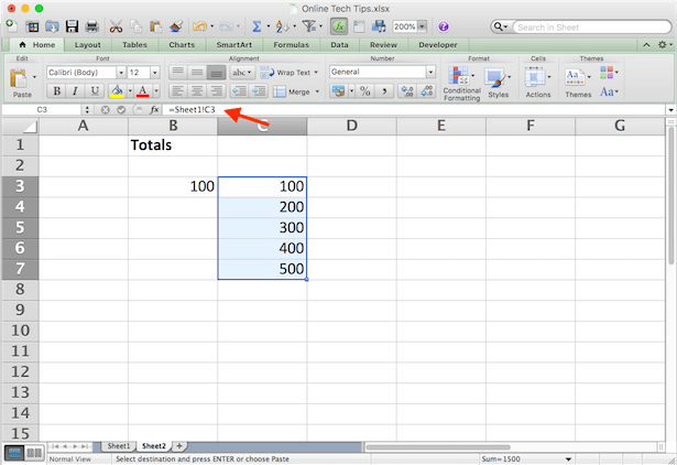
In Sheet2 type an equal symbol (=) into a cell.
Go to the other tab (Sheet1) and click the cell that you want to link to.
Press Enter to complete the formula.

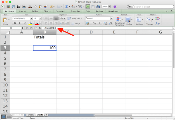
Now, if you click on the cell in Sheet2, you’ll see that Excel writes the path for you in the formula bar.

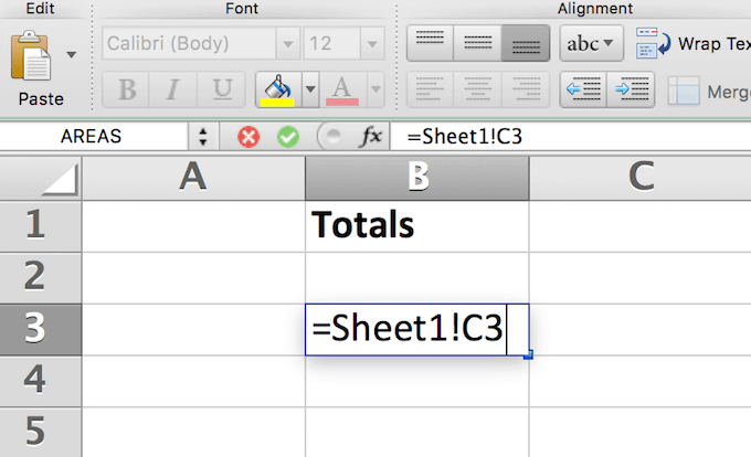
For example, =Sheet1!C3, where Sheet1 is the name of the sheet, C3 is the cell you’re linking to, and the exclamation mark (!) is used as a separator between the two.

Using this approach, you can link manually without leaving the original worksheet at all. Just type the reference formula directly into the cell.

Note: If the sheet name contains spaces (for example Sheet 1), then you need to put the name in single quotation marks when typing the reference into a cell. Like =’Sheet 1′!C3. That’s why it’s sometimes easier and more reliable to let Excel write the reference formula for you.

How to Link a Range of Cells

Another way you can link cells in Excel is by linking a whole range of cells from different Excel tabs. This is useful when you need to store the same data in different sheets without having to edit both sheets.

In order to link more than one cell in Excel, follow these steps.

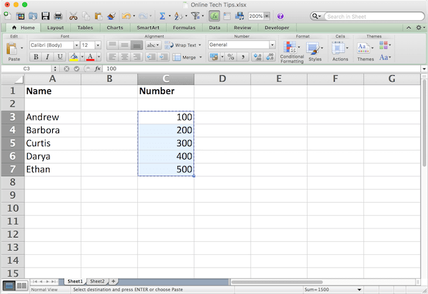
In the original tab with data (Sheet1), highlight the cells that you want to reference.
Copy the cells (Ctrl/Command + C, or right click and choose Copy).
Go to the other tab (Sheet2) and click on the cell (or cells) where you want to place the links.

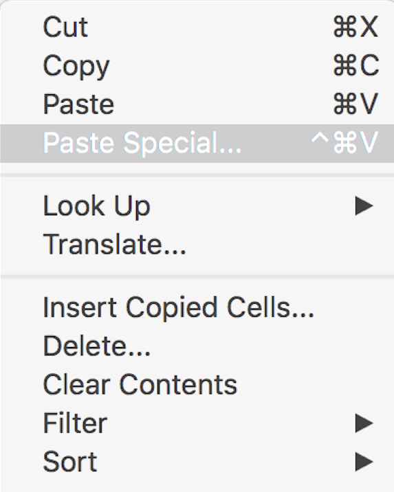
Right click on the cell(-s) and select Paste Special…

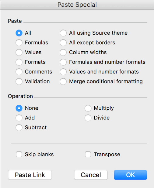
At the bottom left corner of the menu choose Paste Link.

When you click on the newly linked cells in Sheet2 you can see the references to the cells from Sheet1 in the formula tab. Now, whenever you change the data in the chosen cells in Sheet1, it will automatically change the data in the linked cells in Sheet2.

How to Link a Cell With a Function

Linking to a cluster of cells can be useful when you do summations and want to keep them on a sheet separate from the original raw data.

Let’s say you need to write a SUM function in Sheet2 that will link to a number of cells from Sheet1. In order to do that, go to Sheet2 and click on the cell where you want to place the function. Write the function as normal, but when it comes to choosing the range of cells, go to the other sheet and highlight them as described above.

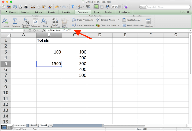
You will have =SUM(Sheet1!C3:C7), where the SUM function sums the contents from cells C3:C7 in Sheet1. Press Enter to complete the formula.

How to Link Cells From Different Excel Files

The process of linking between different Excel files (or workbooks) is virtually the same as above. Except, when you paste the cells, paste them in a different spreadsheet instead of a different tab. Here’s how to do it in 4 easy steps.

Open both Excel documents.
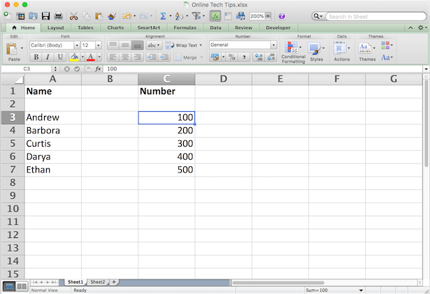
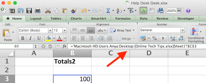
In the second file (Help Desk Geek), choose a cell and type an equal symbol (=).
Switch to the original file (Online Tech Tips), and click on the cell that you want to link to.
Press Enter to complete the formula.

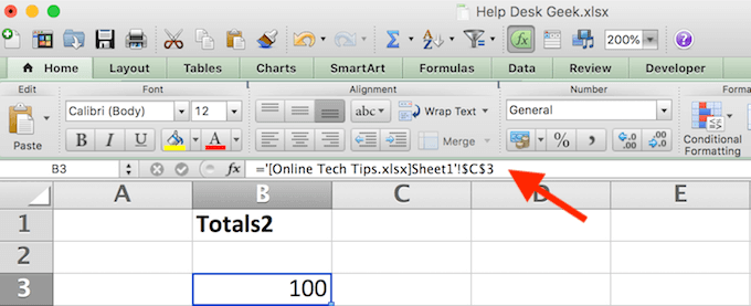
Now the formula for the linked cell also has the other workbook name in square brackets.

If you close the original Excel file and look at the formula again, you will see that it now also has the entire document’s location. Meaning that if you move the original file that you linked to another place or rename it, the links will stop working. That’s why it’s more reliable to keep all the important data in the same Excel file.

Become a Pro Microsoft Excel User

Linking cells between sheets is only one example of how you can filter data in Excel and keep your spreadsheets organized. Check out some other Excel tips and tricks that we put together to help you become an advanced user.

What other neat Excel lifehacks do you know and use? Do you know any other creative ways to link cells in Excel? Share them with us in the comment section below.

Источник

Create an external reference between cells in different workbooks

Create a link to a worksheet in the same workbook

Need more help?

See Also

Need more help?

HYPERLINK function

Description

Syntax

Examples

Create an external reference (link) to a cell range in another workbook

Create an external reference between cells in different workbooks

Create a link to a worksheet in the same workbook

Need more help?

Create or change a cell reference

Need more help?

Linking a range of cells

Option 1: Using Paste Link

Option 2: Create a link manually

Identifying linked cells

Things You Should Know

Video

About This Article

Is this article up to date?

Why Link Cell Data in Excel

How to Link Two Single Cells

How to Link a Range of Cells

How to Link a Cell With a Function

How to Link Cells From Different Excel Files

Become a Pro Microsoft Excel User