How do i add numbers in excel

Adding and subtracting in Excel is easy; you just have to create a simple formula to do it. Just remember that all formulas in Excel begin with an equal sign (=), and you can use the formula bar to create them.

Add two or more numbers in one cell

1. Click any blank cell, and then type an equal sign (=) to start a formula.

2. After the equal sign, type a few numbers separated by a plus sign (+).

   For example, 50+10+5+3.

3. Press RETURN .

   If you use the example numbers, the result is 68.

   Notes: 

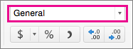
   • If you see a date instead of the result that you expected, select the cell, and then on the Home tab, select General.

   • 

Add numbers using cell references

A cell reference combines the column letter and row number, such as A1 or F345. When you use cell references in a formula instead of the cell value, you can change the value without having to change the formula.

1. Type a number, such as 5, in cell C1. Then type another number, such as 3, in D1.

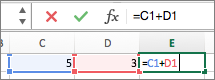
2. In cell E1, type an equal sign (=) to start the formula.

3. After the equal sign, type C1+D1.

4. Press RETURN .

   

   If you use the example numbers, the result is 8.

   Notes: 

   • If you change the value of C1 or D1 and then press RETURN , the value of E1 will change, even though the formula did not.

   • If you see a date instead of the result that you expected, select the cell, and then on the Home tab, select General.

Get a quick total from a row or column

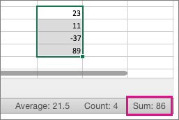
1. Type a few numbers in a column, or in a row, and then select the range of cells that you just filled.

2. On the status bar, look at the value next to Sum. The total is 86.

   

Subtract two or more numbers in a cell

1. Click any blank cell, and then type an equal sign (=) to start a formula.

2. After the equal sign, type a few numbers that are separated by a minus sign (-).

   For example, 50-10-5-3.

3. Press RETURN .

   If you use the example numbers, the result is 32.

Subtract numbers using cell references

A cell reference combines the column letter and row number, such as A1 or F345. When you use cell references in a formula instead of the cell value, you can change the value without having to change the formula.

1. Type a number in cells C1 and D1.

   For example, a 5 and a 3.

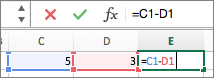
2. In cell E1, type an equal sign (=) to start the formula.

3. After the equal sign, type C1-D1.

   

4. Press RETURN .

   If you used the example numbers, the result is 2.

   Notes: 

   • If you change the value of C1 or D1 and then press RETURN , the value of E1 will change, even though the formula did not.

   • If you see a date instead of the result that you expected, select the cell, and then on the Home tab, select General.

Add two or more numbers in one cell

1. Click any blank cell, and then type an equal sign (=) to start a formula.

2. After the equal sign, type a few numbers separated by a plus sign (+).

   For example, 50+10+5+3.

3. Press RETURN .

   If you use the example numbers, the result is 68.

   Note: If you see a date instead of the result that you expected, select the cell, and then on the Home tab, under Number, click General on the pop-up menu.

Add numbers using cell references

A cell reference combines the column letter and row number, such as A1 or F345. When you use cell references in a formula instead of the cell value, you can change the value without having to change the formula.

1. Type a number, such as 5, in cell C1. Then type another number, such as 3, in D1.

2. In cell E1, type an equal sign (=) to start the formula.

3. After the equal sign, type C1+D1.

4. Press RETURN .

   

   If you use the example numbers, the result is 8.

   Notes: 

   • If you change the value of C1 or D1 and then press RETURN , the value of E1 will change, even though the formula did not.

   • If you see a date instead of the result that you expected, select the cell, and then on the Home tab, under Number, click General on the pop-up menu.

Get a quick total from a row or column

1. Type a few numbers in a column, or in a row, and then select the range of cells that you just filled.

2. On the status bar, look at the value next to Sum=. The total is 86.

   

   If you don’t see the status bar, on the View menu, click Status Bar.

Subtract two or more numbers in a cell

1. Click any blank cell, and then type an equal sign (=) to start a formula.

2. After the equal sign, type a few numbers that are separated by a minus sign (-).

   For example, 50-10-5-3.

3. Press RETURN .

   If you use the example numbers, the result is 32.

Subtract numbers using cell references

A cell reference combines the column letter and row number, such as A1 or F345. When you use cell references in a formula instead of the cell value, you can change the value without having to change the formula.

1. Type a number in cells C1 and D1.

   For example, a 5 and a 3.

2. In cell E1, type an equal sign (=) to start the formula.

3. After the equal sign, type C1-D1.

   

4. Press RETURN .

   If you used the example numbers, the result is -2.

   Notes: 

   • If you change the value of C1 or D1 and then press RETURN , the value of E1 will change, even though the formula did not.

   • If you see a date instead of the result that you expected, select the cell, and then on the Home tab, under Number, click General on the pop-up menu.

See also

Calculating operators and order of operations

Add or subtract dates

Subtract times

Select a cell next to the numbers you want to sum, click AutoSum on the Home tab, press Enter, and you’re done. When you click AutoSum, Excel automatically enters a formula (that uses the SUM function) to sum the numbers.

Type 1 into a cell that you want to start the numbering, then drag the autofill handle at the right-down corner of the cell to the cells you want to number, and click the fill options to expand the option, and check Fill Series, then the cells are numbered. See screenshot.

How do I auto number a column in Excel?

Fill a column with a series of numbers

1. Select the first cell in the range that you want to fill.
2. Type the starting value for the series.
3. Type a value in the next cell to establish a pattern.
4. Select the cells that contain the starting values.
5. Drag the fill handle.

How do you autofill numbers in sheets?

Use autofill to complete a series

1. On your computer, open a spreadsheet in Google Sheets.
2. In a column or row, enter text, numbers, or dates in at least two cells next to each other.
3. Highlight the cells. You’ll see a small blue box in the lower right corner.
4. Drag the blue box any number of cells down or across.

How do you do numbering?

Practice: Use the Numbering Toolbar Button

1. Click the Numbering button on the Formatting toolbar.
2. Type some text and press ENTER.
3. Type several additional items pressing ENTER after each item.
4. Press ENTER twice to turn off numbering.
5. Click the Numbering button to continue with the next sequential number in the list.

How do you create a numbered list?

To start a numbered list, type 1, a period (.), a space, and some text. Then press Enter. Word will automatically start a numbered list for you. Type* and a space before your text, and Word will make a bulleted list.

How do I make a numbered list in numbers?

In the Format sidebar, click the Text tab, then click the Style button near the top of the sidebar. Click the disclosure arrow next to Bullets & Lists, then click the pop-up menu below Bullets & Lists and choose Numbers.

How can you make a numbered list?

To create a numbered list:

1. Select the text you want to format as a list.
2. On the Home tab, click the drop-down arrow next to the Numbering command. A menu of numbering styles will appear.
3. Move the mouse over the various numbering styles.
4. The text will format as a numbered list.

How do you add cells in sheets?

Add more than one row, column, or cell

1. On your computer, open a spreadsheet in Google Sheets.
2. Highlight the number of rows, columns, or cells you want to add. To highlight multiple items:
3. Right-click the rows, columns, or cells.
4. From the menu that appears, select Insert [Number] or Insert cells. For example:

How do you fill down in Excel?

Simply do the following:

1. Select the cell with the formula and the adjacent cells you want to fill.
2. Click Home > Fill, and choose either Down, Right, Up, or Left. Keyboard shortcut: You can also press Ctrl+D to fill the formula down in a column, or Ctrl+R to fill the formula to the right in a row.

How do I fill rows in Excel without dragging?

The regular way of doing this is: Enter 1 in cell A1. Enter 2 in cell A2. Select both the cells and drag it down using the fill handle.
Quickly Fill Numbers in Cells without Dragging

1. Enter 1 in cell A1.
2. Go to Home –> Editing –> Fill –> Series.
3. In the Series dialogue box, make the following selections:
4. Click OK.

What is a numbered text?

Both forms provide a unique identifier for a block of text. With numbered text, the last identifier also conveys how many blocks were in the list. With outline-numbered text, the items are in a well-ordered hierarchy.

How do I continue number 1.1 in Word?

Number your headings

1. Open your document that uses built-in heading styles, and select the first Heading 1.
2. On the Home tab, in the Paragraph group, choose Multilevel List.
3. Under List Library, choose the numbering style you would like to use in your document.

How do I set up automatic numbering?

Turn on or off automatic bullets or numbering

1. Go to File > Options > Proofing.
2. Select AutoCorrect Options, and then select the AutoFormat As You Type tab.
3. Select or clear Automatic bulleted lists or Automatic numbered lists.
4. Select OK.

Which tag is used to create a numbered list?

: The Ordered List element. The
HTML element represents an ordered list of items — typically rendered as a numbered list.

How do I insert sequential numbers in Word?

As an example of how you can do this, follow these steps:

1. Position the insertion point where you want the sequential number to appear.
2. Press Ctrl+F9 to insert field braces.
3. Type “seq NumList” (without the quote marks).
4. Press F9 to update the field information.

How do you modify a numbered list?

Change the numbering in a numbered list

1. Double-click the numbers in the list. The text won’t appear selected.
2. Right-click the number you want to change.
3. Click Set Numbering Value.
4. In the Set value to: box, use the arrows to change the value to the number you want.

What is the shortcut key for numbering?

in most Google Tools: Click CTRL (Command on Mac) + Shift + 7 for Numbering. Click it again to undo numbering. Click CTRL (Command on Mac) + Shift + 8 for Bullets.

How do I insert a dot symbol?

Open your document and put the cursor right where you desire to insert the bullet point symbol [•]. On your keyboard, locate the Alt Key. Press it and hold as you type the Alt code 0149. After typing the Alt code 0149, release the Alt key, and the bullet point symbol [•] will be inserted into your word document.

How do you do math in Google Sheets?

To do math in a Google spreadsheet, follow these steps:

1. Type an equals sign in a cell (=)
2. Type a number, or a cell reference (of a cell that contains a number)
3. Then use one of the following mathematical operators + (Plus), – (Minus), * (Multiply), / (Divide)
4. Type another number or cell reference.
5. Press enter.

How do I add a formula to a column in Google Sheets?

Here’s how to enter a formula in Google sheets. Double click on the cell where you want your formula, and then type “=” without quotes, followed by the formula. Press Enter to save formula or click on another cell.

Last Updated on July 23, 2022

Microsoft Excel is used by businesses around the world to manage and organize data into spreadsheets. There are multiple tricks that you can perform in this program to make basic data entry much faster and easier. 

In this guide, we will be teaching you a few tricks involving adding numbers to cells in Excel. This will include automatically adding numbers that follow a set sequence to your cells, or copying the same number across multiple cells.

We will also tell you how to add numbers in different cells together.

How To Automatically Add Numbers To Cells

Clicking on each individual cell in your spreadsheet to add numbers is a slow and tedious process. Thankfully, there are ways to automatically add numbers to your cells with a few simple steps, which will be covered below.

Conclusion

Anyone who has ever worked with Excel will likely be working with a lot of numbers. With the tips we have described in this article, you will be able to add numbers in Excel and auto-number your cells in a matter of seconds. 

Not only will this help you to save time, but it will also make you much more efficient when using this program. If you found this article helpful, then why not share it with your friends or co-workers.

You can also check out our other guides to discover more awesome tips for using Excel.

Watch Video – 7 Quick and Easy Ways to Number Rows in Excel

When working with Excel, there are some small tasks that need to be done quite often. Knowing the ‘right way’ can save you a great deal of time.

One such simple (yet often needed) task is to number the rows of a dataset in Excel (also called the serial numbers in a dataset).

Now if you’re thinking that one of the ways is to simply enter these serial number manually, well – you’re right!

But that’s not the best way to do it.

Imagine having hundreds or thousands of rows for which you need to enter the row number. It would be tedious – and completely unnecessary.

There are many ways to number rows in Excel, and in this tutorial, I am going to share some of the ways that I recommend and often use.

Of course, there would be more, and I will be waiting – with a coffee – in the comments area to hear from you about it.

How to Number Rows in Excel

The best way to number the rows in Excel would depend on the kind of data set that you have.

For example, you may have a continuous data set that starts from row 1, or a dataset that start from a different row. Or, you might have a dataset that has a few blank rows in it, and you only want to number the rows that are filled.

You can choose any one of the methods that work based on your dataset.

1] Using Fill Handle

Fill handle identifies a pattern from a few filled cells and can easily be used to quickly fill the entire column.

Suppose you have a dataset as shown below:

Here are the steps to quickly number the rows using the fill handle:

Note that Fill Handle automatically identifies the pattern and fill the remaining cells with that pattern. In this case, the pattern was that the numbers were getting incrementing by 1.

In case you have a blank row in the dataset, fill handle would only work till the last contiguous non-blank row.

Also, note that in case you don’t have data in the adjacent column, double-clicking the fill handle would not work. You can, however, place the cursor on the fill handle, hold the right mouse key and drag down. It will fill the cells covered by the cursor dragging.

2] Using Fill Series

While Fill Handle is a quick way to number rows in Excel, Fill Series gives you a lot more control over how the numbers are entered.

Suppose you have a dataset as shown below:

Here are the steps to use Fill Series to number rows in Excel:

This will instantly number the rows from 1 to 26.

Using ‘Fill Series’ can be useful when you’re starting by entering the row numbers. Unlike Fill Handle, it doesn’t require the adjacent columns to be filled already.

Even if you have nothing on the worksheet, Fill Series would still work.

Note: In case you have blank rows in the middle of the dataset, Fill Series would still fill the number for that row.

3] Using the ROW Function

You can also use Excel functions to number the rows in Excel.

In the Fill Handle and Fill Series methods above, the serial number inserted is a static value. This means that if you move the row (or cut and paste it somewhere else in the dataset), the row numbering will not change accordingly.

This shortcoming can be tackled using formulas in Excel.

You can use the ROW function to get the row numbering in Excel.

To get the row numbering using the ROW function, enter the following formula in the first cell and copy for all the other cells:

=ROW()-1

The ROW() function gives the row number of the current row. So I have subtracted 1 from it as I started from the second row onwards. If your data starts from the 5th row, you need to use the formula =ROW()-4.

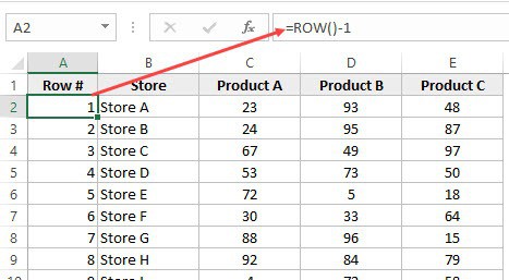
The best part about using the ROW function is that it will not screw up the numberings if you delete a row in your dataset.

Since the ROW function is not referencing any cell, it will automatically (or should I say AutoMagically) adjust to give you the correct row number. Something as shown below:

Note that as soon as I delete a row, the row numbers automatically update.

Again, this would not take into account any blank records in the dataset. In case you have blank rows, it will still show the row number.

You can use the following formula to hide the row number for blank rows, but it would still not adjust the row numbers (such that the next row number is assigned to the next filled row).

IF(ISBLANK(B2),"",ROW()-1)

4] Using the COUNTA Function

If you want to number rows in a way that only the ones that are filled get a serial number, then this method is the way to go.

It uses the COUNTA function that counts the number of cells in a range that are not empty.

Suppose you have a dataset as shown below:

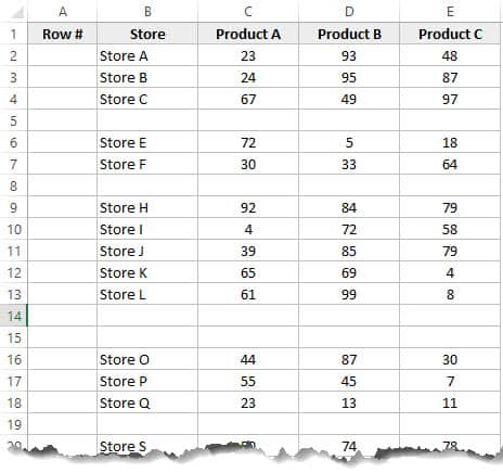
Note that there are blank rows in the above-shown dataset.

Here is the formula that will number the rows without numbering the blank rows.

=IF(ISBLANK(B2),"",COUNTA($B$2:B2))

The IF function checks whether the adjacent cell in column B is empty or not. If it’s empty, it returns a blank, but if it’s not, it returns the count of all the filled cells till that cell.

5] Using SUBTOTAL For Filtered Data

Sometimes, you may have a huge dataset, where you want to filter the data and then copy and paste the filtered data into a separate sheet.

If you use any of the methods shown above so far, you will notice that the row numbers remain the same. This means that when you copy the filtered data, you will have to update the row numbering.

In such cases, the SUBTOTAL function can automatically update the row numbers. Even when you filter the data set, the row numbers will remain intact.

Let me show you exactly how it works with an example.

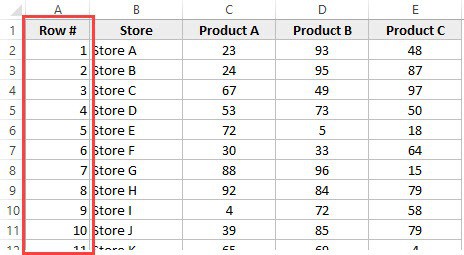
Suppose you have a dataset as shown below:

If I filter this data based on Product A sales, you will get something as shown below:

Note that the serial numbers in Column A are also filtered. So now, you only see the numbers for the rows that are visible.

While this is the expected behavior, in case you want to get a serial row numbering – so that you can simply copy and paste this data somewhere else – you can use the SUBTOTAL function.

Here is the SUBTOTAL function that will make sure that even the filtered data has continuous row numbering.

=SUBTOTAL(3,$B$2:B2)

The 3 in the SUBTOTAL function specifies using the COUNTA function. The second argument is the range on which COUNTA function is applied.

The benefit of the SUBTOTAL function is that it dynamically updates when you filter the data (as shown below):

Note that even when the data is filtered, the row numbering update and remains continuous.

6] Creating an Excel Table

Excel Table is a great tool that you must use when working with tabular data. It makes managing and using data a lot easier.

This is also my favorite method among all the techniques shown in this tutorial.

Let me first show you the right way to number the rows using an Excel Table:

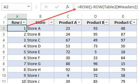
Note that in the formula above, I have used Table2, as that is the name of my Excel table. You can replace Table2 with the name of the table you have.

There are some added benefits of using an Excel Table while numbering rows in Excel:

1. Since Excel Table automatically inserts the formula in the entire column, it works when you insert a new row in the Table. This means that when you insert/delete rows in an Excel Table, the row numbering would automatically update (as shown below).
2. If you add more rows to the data, Excel Table would automatically expand to include this data as a part of the table. And since the formulas automatically update in the calculated columns, it would insert the row number for the newly inserted row (as shown below).

7] Adding 1 to the Previous Row Number

This is a simple method that works.

The idea is to add 1 to the previous row number (the number in the cell above). This will make sure that subsequent rows get a number that is incremented by 1.

Suppose you have a dataset as shown below:

Here are the steps to enter row numbers using this method:

• In the cell in the first row, enter 1 manually. In this case, it’s in cell A2.
• In cell A3, enter the formula, =A2+1
• Copy and paste the formula for all the cells in the column.

The above steps would enter serial numbers in all the cells in the column. In case there are any blank rows, this would still insert the row number for it.

Also note that in case you insert a new row, the row number would not update. In case you delete a row, all the cells below the deleted row would show a reference error.

These are some quick ways you can use to insert serial numbers in tabular data in Excel.

In case you are using any other method, do share it with me in the comments section.

You May Also Like the Following Excel Tutorials:

• Delete Blank Rows in Excel (with and without VBA).
• How to Insert Multiple Rows in Excel (4 Methods).
• How to Split Multiple Lines in a Cell into a Separate Cells / Columns.
• 7 Amazing Things Excel Text to Columns Can Do For You.
• Highlight EVERY Other ROW in Excel.
• How to Compare Two Columns in Excel.
• Insert New Columns in Excel