

on
March 11, 2019, 3:32 AM PDT
Use Excel to calculate the hours worked for any shift
With Microsoft Excel, you can create a worksheet that figures the hours worked for any shift. Follow these step-by-step instructions.
We may be compensated by vendors who appear on this page through methods such as affiliate links or sponsored partnerships. This may influence how and where their products appear on our site, but vendors cannot pay to influence the content of our reviews. For more info, visit our Terms of Use page.
To calculate in Excel how many hours someone has worked, you can often subtract the start time from the end time to get the difference. But if the work shift spans noon or midnight, simple subtraction won’t cut it.
However, you can easily create an Excel worksheet that correctly figures the hours worked for any shift.
LEARN MORE: Office 365 Consumer pricing and features
Follow these steps:
- In A1, enter Time In.
- In B1, enter Time Out.
- In C1, enter Hours Worked.
- Select A2 and B2, and press [Ctrl]1 to open the Format Cells dialog box.
- On the Number tab, select Time from the Category list box, choose 1:30 PM from the Type list box, and click OK.
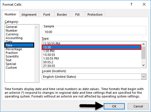
- Right-click C2, and select Format Cells.
- On the Number tab, select Time from the Category list box, choose 13:30 from the Type list box, and click OK.
- In C2, enter the following formula:
=IF(B2<A2,B2+1,B2)-A2
If you enter 11:00 PM as the Time In and enter 7:00 AM as the Time Out, Excel will display 8, the correct number of hours worked.
A bonus Microsoft Excel tip
From the article 10 things you should never do in Excel by Susan Harkins:
Rely on multiple links: Links between two workbooks are common and useful. But multiple links where values in workbook1 depend on values in workbook2, which links to workbook3, and so on, are hard to manage and unstable. Users forget to close files, and sometimes they even move them. If you’re the only person working with those linked workbooks, you might not run into trouble, but if other users are reviewing and modifying them, you’re asking for trouble. If you truly need that much linking, you might consider a new design.
This bonus Excel tip is also available in the free PDF 30 things you should never do in Microsoft Office.
Editor’s note on March 11, 2019: This Excel article was first published in June 2005. Since then, we have included a video tutorial, added a bonus tip, and updated the related resources.
Also See
-
How to add a drop-down list to an Excel cell
(TechRepublic) -
Tap into the power of Excel’s data validation feature (free PDF)
(TechRepublic) -
You’ve been using Excel wrong all along (and that’s OK)
(ZDNet) -
A cheatsheet of Excel shortcuts that make inserting data faster
(TechRepublic) -
Six clicks: Excel power tips to make you an instant expert
(ZDNet) -
10 things you should never do in Excel
(TechRepublic)
-
Microsoft
-
Software
Single simple formula to calculate the hours worked for a day shift or night shift and including lunch and all breaks in the calculation.
This tutorial will show you the simple formula that you can use for this and tell you how you can customize it to work for your situation, where you might have more breaks or fewer breaks for which to account.
(Some times in this tutorial are presented using the 24 hour clock, or military time, but that doesn’t change anything in regard to the formulas or their outcomes.)
Sections:
Magic Formula to Calculate Hours Worked
Simple Hours Worked
Day Shift Hours Worked with Breaks and Lunch
Night Shift Hours Worked with Breaks and Lunch
Notes
Magic Formula to Calculate Hours Worked
=MOD(Time_Out - Time_In,1)*24Time_Out is when they stopped work for whatever reason.
Time_In is when they started work.
*24 is what changes the time format into a decimal format that is easier to read and can be used in mathematical calculations, such as for wages.
This simple formula is the building block for the rest of the tutorial and works for day and night shifts alike.
Using the MOD function, we are able to seamlessly calculate the number of hours and minutes worked during a day shift, night shift, or over both without the hassel of unmanageably long formulas.
This formula also lets us take breaks and lunch into account; we simply create this formula for each break from work and then subtract that from the total time between the first IN and last OUT of the day.
Everything in this tutorial will be an extension of this formula, basically just adding it again for each IN/OUT section.
Let’s start with a simple example in the next section and work our way up to the full example.
Simple Hours Worked
Note: the easiest way to perform this calculation is also the least useful in the real-world and so I won’t cover it beyond this next sentence. With simple times, you can subtract the OUT time from the IN time to get the result, such as =B1-A1 where A1 has the IN time and B1 has the OUT time. This formula breaks-down very quickly in the real world though, so it won’t be covered here; however, I felt it was important to mention it in this note.
=MOD(C2-B2,1)C2 is the time work stoped. OUT
B2 is the time work started. IN
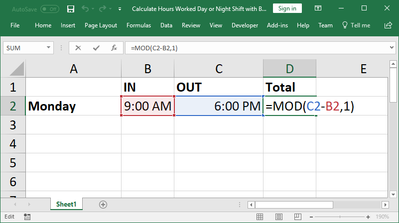
This returns a time like this:
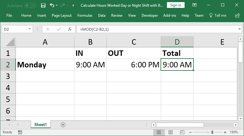
Get Hours from the Time
The current format is still a time format and is not very useful for calculating how much to pay someone, among other considerations, so let’s change the time to hours.
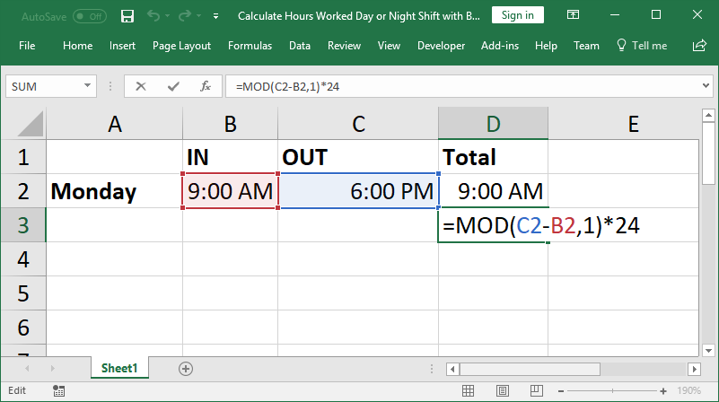
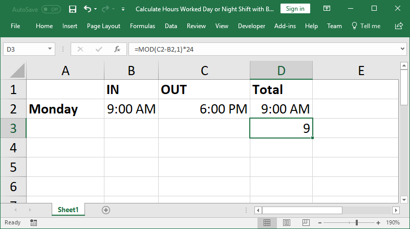
=MOD(C2-B2,1)*24*24 was added to the end of the formula, which multiplies the time by 24. This effectively converts the time into a decimal form.
Now:
8 hours and 30 minutes becomes 8.5
8 hours and 45 minutes becomes 8.75
Etc.
Result:
Problem: Weird Format for the Time
If you get a weird time result when you multiply the time by 24, make sure to change the formatting of the cell to General.
If the format is still set to a time or date format, it will not display correctly.
Hint: Ctrl + Shift + ~ will quickly change all selected cells to the General format.
Wage Calculation
Now that you have hours and decimals for the time someone worked, you can easily use this number to calculation wages or sum hours worked per week or month or year, etc.
Day Shift Hours Worked with Breaks and Lunch
We use one MOD function for each IN/OUT segment and subtract the breaks from the total time worked.
=(MOD(G12-B12,1)-MOD(D12-C12,1)-MOD(F12-E12,1))*24MOD(G12-B12,1) calculates the total time that was worked, using the first time IN and last time OUT.
-MOD(D12-C12,1) calculates the time of the first break. Notice the minus sign in front of this MOD; that is because we are subtracting this break from the total time worked in the day.
-MOD(F12-E12,1) calculates the time of the second break. Notice the minus sign in front of this MOD; that is because we are subtracting this break from the total time worked in the day.
*24 this is put on at the end in order to convert the time format into an hour decimal format that is easy to view and use in calculations such as how much to pay someone. It converts something from 8:30 into 8.5 or 8:45 into 8.75, etc.
() remember to enclose all of the MOD functions together within a set of parentheses before multiplying by 24 or the result will be incorrect.
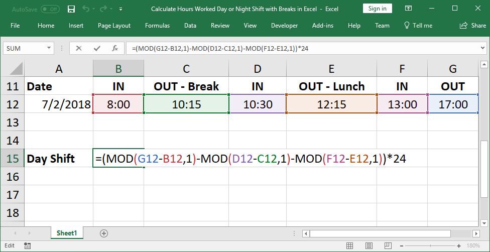
Result:
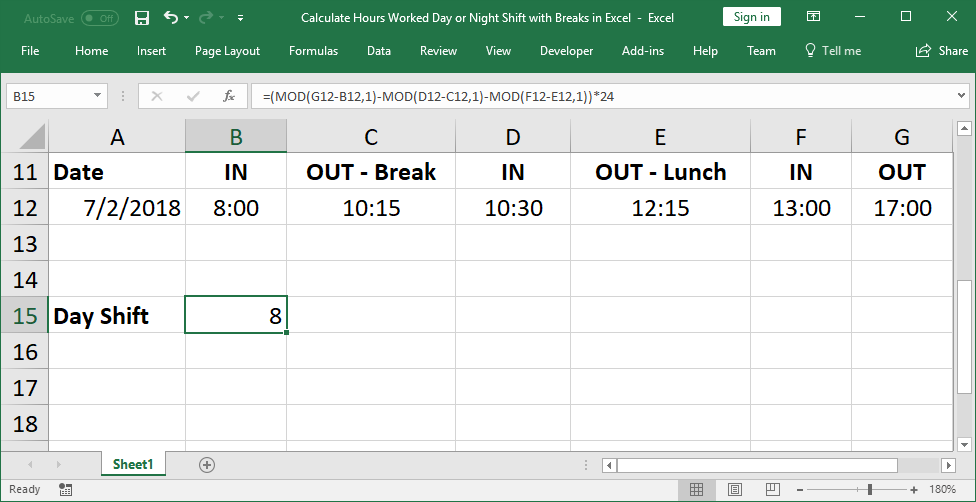
This is the basic formula.
Add or remove as many MOD() chunks as you need in order to account for all of the breaks that someone can take during the day.
Funky Formatting
If the result doesn’t look right, make sure to set the result cell’s formatting to General. You can do this from the Home tab or use the keyboard shortcut Ctrl + Shift + ~.
Night Shift Hours Worked with Breaks and Lunch
This heavenly formula is exactly the same as the one for the day shift!
We use one MOD function for each IN/OUT segment and subtract the breaks from the total time worked.
=(MOD(G13-B13,1)-MOD(D13-C13,1)-MOD(F13-E13,1))*24Cell references have been updated, from the day formula; in Excel I literally just copied the formula down one cell, so the only change was the automatically updating relative cell references.
MOD(G13-B13,1) calculates the total time that was worked, using the first time IN and last time OUT.
-MOD(D13-C13,1) calculates the time of the first break. Notice the minus sign in front of this MOD; that is because we are subtracting this break from the total time worked.
-MOD(F13-E13,1) calculates the time of the second break. Notice the minus sign in front of this MOD; that is because we are subtracting this break from the total time worked.
*24 this is put on at the end in order to convert the time format into an hour decimal format that is easy to view and use in calculations such as how much to pay someone. It converts something from 8:30 into 8.5 or 8:45 into 8.75, etc.
() remember to enclose all of the MOD functions together within a set of parentheses before multiplying by 24 or the result will be incorrect.
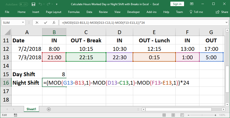
Result:
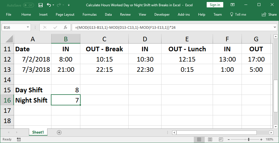
This is the basic formula.
Add or remove as many MOD() chunks as you need in order to account for all of the breaks that someone can take.
Funky Formatting
If the result doesn’t look right, make sure to set the result cell’s formatting to General. You can do this from the Home tab or use the keyboard shortcut Ctrl + Shift + ~.
Notes
There are many different ways to calculate time and hours worked in Excel, but, every single way, when used in the real world, is going to be more complicated and confusing than using the MOD function method exhibited in this tutorial. With the MOD function, everything is simple and logical and easy-to-follow. As such, I didn’t spend time showing you other methods because, in reality, you shouldn’t use any other method for the vast majority of situations.
Use the MOD function, keep the code modular, build on it as needed with required logic, and it will all work out, just give it time!
Download the workbook for this tutorial to view these examples in Excel.
Do you know what all of your employees are working on at every moment of the day?
The answer is probably no. And while that may seem okay at the moment, this lack of knowledge can have negative effects on your business as your company grows, and as control over day-to-day operations moves away from you.
In this article, you will learn:
- How Excel timesheet templates work
- How to create an Excel timesheet template with formulas
- How to calculate hours worked in Excel
- Calculating total hours worked
- Calculating regular work hours
- Calculating overtime hours
- Calculating employee pay with Excel payroll formulas
- Locking timesheets when using Excel
- Best practices on distributing Excel timesheets
- Make the most of out timesheets
- Automate the whole process
Being unable to account for where your team spends their time can cause your business’ productivity and profitability to take a hit. This can lead to stagnation and decline.
One of the simplest and most effective ways of avoiding this is introducing timesheets to your company. Timesheets keep track of all the hours your team works each day, the tasks they worked on, and when they did them. Read more about benefits of time tracking in this post.
In this post, you’ll learn how to work with timesheets in Excel to record your team’s progress more accurately and improve your productivity.
How Excel timesheet templates work
Timesheet templates created in Excel are incredibly flexible and can be adapted to suit the individual needs that your business has. However, the overall way they work remains the same. Good timesheet practice will follow this framework:
- Set up timesheets globally, individually, or on a team-by-team basis
- Distribute among employees
- Use for all work, individual projects, or only for tracking billable hours
- Submit to team leaders or project managers for timesheet approval
- Collect and collate data to gain an understanding of how the business and teams are functioning as a whole
- Monthly timesheet review sessions looking at the bigger picture to spot inefficiencies and room for improvement
Timesheets work by keeping everyone updated with how long an employee spends at work, and the type of work they do. Passing timesheets up the hierarchy chain means that all levels of the company understand what goes on from top to bottom.
Automate time tracking with Hubstaff
Stop wasting time on creating timesheets manually

Creating Excel timesheet templates with formulas
Excel timesheet templates are the simplest way of recording hours, as they require minimal setup time and minimal input from employees.
Let’s take a look at how to use Microsoft Excel for this purpose. We’ve created a video explaining how to create a timesheet in Excel:
Excel allows for several operations within its cells that allow you to create timesheets customized to your team or business. Essentially, just imagine a typical paper time card and its contents, and convert that into digital spreadsheet form.
To start, fill out your sheet with the following information (feel free to modify depending on your company needs):
- Employee information: Name, department, supervisor, rate
- Entry date
- Tasks performed
- Start time and end time
- Regular and overtime hours worked
- Additional notes
You could also customize the sheet by adding colors, or by placing your company logo if you’re planning on printing and archiving it. Your timesheet should look something like this:
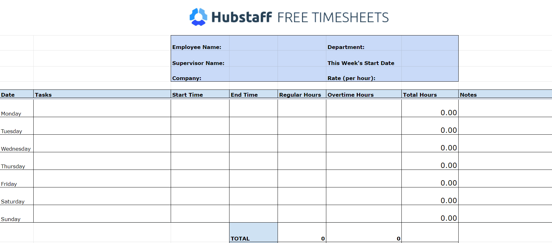
The only columns your team will be filling in will be the Date, Tasks, Start Time, End Time, and Notes columns. You can place formulas within the Regular Hours, Overtime Hours, and Total Hours columns that will automatically calculate the hours based on their start and end time entries.
How to calculate hours worked in Excel
Calculating total hours worked
Calculating the daily hours worked by your team with a spreadsheet isn’t difficult. To start things off, set the Total Hours column to count the number of hours between the start time and end time entries. This can be done by inputting the following formula:
- Total Hours = (End Time – Start Time) * 24

It’s necessary to multiply by 24 because Excel registers a whole day as a value of 1 (e.g. 12 hours will result in a value of 0.5).
Calculating regular hours worked
After the Total Hours, you’ll need a formula for your Regular Hours column. This will depend on how many maximum hours your team is allowed to work before it’s considered overtime. Your formula will look like this:
- Regular Hours = IF (Total Hours >= (max regular hours), (max regular hours), Total Hours)

In the example above, 8 is the maximum number of regular hours your team can work before going into overtime. The Regular Hours cell will only accept a maximum value of 8; if the total number of hours goes beyond that, the excess should go to the Overtime Hours cell.
Be more productive with automated timesheets
Calculating overtime hours
Below is the formula for overtime hours:
- Overtime Hours = IF (Total Hours <= max regular hours, 0, (Total Hours – max regular hours))

Based on the start and end time entries, any hours your team worked beyond the daily maximum will automatically be reflected in the Overtime Hours column. This way, you could easily check for unpermitted overtime work, and calculate their overtime pay with increased accuracy.
Calculating employee pay with Excel payroll formulas
After you’ve set up your timesheets to compute regular and overtime hours, you can use them to calculate your team’s pay. This can be done by multiplying their rates with the total number of both regular and overtime hours.
First, use the following formula to count the total number of regular and overtime hours.
- Total Hours = SUM (first row:last row)

Use the same formula for the Overtime and Total Hours columns. For the amount earned, use the following:
- Pay = hours worked * hourly rate

In the example above, the hourly rate is $10 per hour. Use the same formula for the total number of overtime hours worked, or use a different value for the hourly rate if you have specific overtime policies.
To get the total amount earned, simply add the totals of the regular and overtime hours.
- Total Amount Earned = Regular Amount Earned + Overtime Amount Earned
After that, you’re all set. All your team has to do is put in the time they started and stopped working, and the template will do the rest.

Locking timesheets
After timesheets have been submitted, it’s important to limit access for anyone other than authorized managers. This adds an additional layer of security against timesheet fraud, overpayments, and accidental edits to entries.
Formulas aren’t necessary for locking your timesheets. An easy way to do this would be to have your team upload their timesheets at the end of each week to your company’s shared drive. Or, you could create the timesheets directly there if you’re using a file storage and collaboration platform like Google Drive.
The best way to “lock” timesheets is to have your team upload them to one shared folder. Once all of them are turned in, move them to a separate folder accessible only by you, team leaders, and project managers. This prevents the timesheets from being edited by your team after they are submitted.
Distribute timesheets
Once your Excel timesheet template is prepared, it’s time to implement it across all of your teams. The process is straightforward, but here are some things to keep in mind:
- Customize templates and make adjustments to suit individual projects or variations in employee billing/hourly rates
- Turn your Excel timesheet into a PDF. PDFs can be customized for each employee, printed off, and handed in each week or month
- Turn your Excel timesheet into a Word document. Word documents can be managed on a computer and then uploaded to a file-sharing service at the end of the month or another defined period
- Turn your timesheet into a Google spreadsheet that’s worked on collaboratively. There’s no need to worry about employees doctoring their times or the times of others as Google tracks changes made to the document
- Distribute to employees using one of the methods noted above
- Track the data: Depending on the option used, you can either collate data on a monthly basis and then analyze, or check-in periodically
- Analyze and refine: Make changes to workflows, team structures, and resource distribution based on feedback and data collected by timesheets
One thing to remember is that discipline and consistency are absolutely necessary for timesheets to have maximum effect, but they pay off. After a while, you’ll start to notice your teams’ productivity start rising, and your business’ overall performance improving.
An easier way to track hours
Automatic time tracking, productivity measurement, detailed reports, and more

How to make the most of timesheet templates
The key to making the most out of timesheet templates is following a rigid process, and ensuring that your employees fill them out regularly.
The benefits that timesheet templates have to offer your business (in terms of cost-saving, waste elimination, and data gathering) mean that they are an invaluable business tool that should always be used to the greatest effect. Here are some guidelines to make this happen:
Make employees fill timesheets out honestly, and on a regular basis
Employees should fill out their timesheets multiple times each day, and should make sure that they are completely honest with the time that they input.
One of the benefits of timesheets is that they help to pinpoint inefficiencies and roadblocks that stop your employees from working effectively. You can only identify these when your employees have filled out their timesheets honestly, as any made-up entries will skew the data.
Closely monitor timesheets to spot trends
As a leader within your company, you and other managers should closely monitor the timesheets that employees submit so that you can identify trends (both positive and negative). And, so that you can stay constantly informed of what’s going on in your business.
To do this effectively, spend some time each week looking back on the timesheet information, identifying areas of low (and high) productivity across the board, and then try to match up these areas to events that happened during the week.
Doing this often will help you to continuously improve your business.
Hold regular review sessions with team leaders and managers to deconstruct business’ performance and productivity
To make sure that you are getting the best out of your employees, hold regular sessions to review the performance of individual employees and your business as a whole.
Having regular review sessions means that even if you aren’t heavily involved with what goes on in your company on a day-to-day basis, you’ll still have a great understanding of how things are actually running and that you are positioned to make informed decisions about your company’s future.
Continuously refine your company’s processes and workflows
Having all of the data about how your employees work means that you can make informed decisions that refine workflows and change your company’s processes. Both of these can make your company more cost-efficient and more productive.
Automate the whole process with Hubstaff’s online timesheets

Hubstaff is a time tracking solution that allows you to streamline timesheets and time management. It tracks all of your team’s work hours, and the tasks they work on, and automatically generates detailed and accurate timesheets.
Instead of entering hours into a timesheet template, Hubstaff tracks time toward specific projects and tasks with a simple start and stop feature available through desktop, web, or mobile apps.
With Hubstaff, your team doesn’t have to note what time they have arrived in the office or started working, or what tasks they spent time on. They can start tracking their time and the task with just the click of a button. Hubstaff will handle everything else from timesheet creation to payroll processing.
Managers can get daily timesheets emailed directly to them, see how much of a budget has been used, set hourly limits for team members, and review and approve timesheets all from one central dashboard.
Compared to timesheet templates, Hubstaff offers a higher level of accuracy because you can turn on features including app and URL tracking, random screen capture while the timer is running, activity rates, and more. With Hubstaff, there’s no question about what was worked on when.
Finally, you can use the hours tracked and pay rates to automatically issue payroll to your team. The same goes for client invoices; just review timesheets at the end of each pay period, set bill rates, and you can send invoices much sooner.
Power up your workday
Reach your goals faster with time tracking and work management.

Are you ready to start using timesheets?
Timesheets, when used correctly, are hugely powerful tools that can help to transform your business for the better.
They can dramatically increase productivity, make it easier for your employees to motivate themselves, and make your business run more smoothly.
To get started implementing timesheets into your business, you can download timesheet templates that we prepared, or create one specifically tailored for your business with a spreadsheet app and our guide above.
Alternatively, you can use Hubstaff to automate the whole process, and not worry about forgetting to note what time you clocked in or out.
Whatever your choice is, we’d like to know if you use timesheet templates in your organization, and how it has contributed to your team’s success. Do you have any go-to templates you’ve been using for years, or software tools that might be helpful to other business owners as well? Let us hear about it in the comments below.
This post was originally published September 15, 2016, and updated August 2019.
Subscribe to the Hubstaff blog for more posts like this
Contents
- 1 How do you sum HH mm/s in Excel?
- 2 How do you calculate total hours worked in a month in Excel?
- 3 What is the easiest way to calculate hours worked?
- 4 How do you calculate hours worked?
- 5 How do you sum amounts in Excel?
- 6 How do I calculate time duration in Excel?
- 7 How do I add 24 hours to a time in Excel?
- 8 How do you calculate pay hours?
- 9 Can you SUM text in Excel?
- 10 How do you SUM and MaX in Excel?
- 11 How do I calculate hours and minutes in Excel for payroll?
- 12 How do I add 8 hours to a time in Excel?
- 13 How do I add 6 hours to a time in Excel?
- 14 How do you calculate your hours and minutes worked?
- 15 How do I calculate payroll time in Excel?
- 16 How do you sum and deduct in Excel?
How do you sum HH mm/s in Excel?
In the Format Cells dialog box, go to the Number tab, select Custom in the Category box, then enter [HH]:MM or [HH]:MM:SS into the Type box, and finally click the OK button. See screenshot: Now the result of summing times is displayed over 24 hours as below screenshot shown.
How do you calculate total hours worked in a month in Excel?
How to calculate working hours per month in Excel?
- Calculate total working hours per month with formulas.
- Enter this formula: =NETWORKDAYS(A2,B2) * 8 into a blank cell where you want to put the result, and then press Enter key, and you will get a date format cell as following screenshot shown:
What is the easiest way to calculate hours worked?
How to calculate hours worked
- Determine the start and the end time.
- Convert the time to military time (24 hours)
- Transform the minutes in decimals.
- Subtract the start time from the end time.
- Subtract the unpaid time taken for breaks.
How do you calculate hours worked?
Take your number of minutes and divide by 60.
- Take your number of minutes and divide by 60. In this example your partial hour is 15 minutes:
- Add your whole hours back in to get 41.25 hours. So 41 hours, 15 minutes equals 41.25 hours.
- Multiply your rate of pay by decimal hours to get your total pay before taxes.
How do you sum amounts in Excel?
If you need to sum a column or row of numbers, let Excel do the math for you. Select a cell next to the numbers you want to sum, click AutoSum on the Home tab, press Enter, and you’re done. When you click AutoSum, Excel automatically enters a formula (that uses the SUM function) to sum the numbers. Here’s an example.
How do I calculate time duration in Excel?
Another simple technique to calculate the duration between two times in Excel is using the TEXT function:
- Calculate hours between two times: =TEXT(B2-A2, “h”)
- Return hours and minutes between 2 times: =TEXT(B2-A2, “h:mm”)
- Return hours, minutes and seconds between 2 times: =TEXT(B2-A2, “h:mm:ss”)
How do I add 24 hours to a time in Excel?
To add a desired time interval to a given time, divide the number of hours, minutes, or seconds you want to add by the number of the corresponding unit in a day (24 hours, 1440 minutes, or 86400 seconds), and then add the quotient to the start time.
How do you calculate pay hours?
First, determine the total number of hours worked by multiplying the hours per week by the number of weeks in a year (52). Next, divide this number from the annual salary. For example, if an employee has a salary of $50,000 and works 40 hours per week, the hourly rate is $50,000/2,080 (40 x 52) = $24.04.
Can you SUM text in Excel?
Press Ctrl + Shift + Enter to get the SUM of the required text values as this is an array formula.
How do you SUM and MaX in Excel?
Select a cell which you place the formula at, type this =MaX(20,(SUM(A5:A10))), A5:A10 is the cell range you will sum up, and press Enter.
How do I calculate hours and minutes in Excel for payroll?
Click on cell “A1” and enter the first of your payroll times. Enter the time as “xx:yy” where “xx” is the number of hours worked, and “yy” is the number of minutes worked. Press Enter and Excel will automatically select cell A2. Enter your next payroll time in A2.
How do I add 8 hours to a time in Excel?
In the Formulas Helper dialog box, you need to:
- In the Choose a formula box, select Add hours to date.
- In the Date Time box, select the cell containing the date time you will add or subtract hours from.
- In the Number box, enter the number of hours you want to add or substract.
- Click the OK button.
How do I add 6 hours to a time in Excel?
In Excel, generally, you may use the formulas to add hours, minutes or seconds to the datetime cells. 1. Select the cell next to the first cell of the datetime list, and then type this formula =A2+1/24 into it, press Enter key and drag the auto fill handle over the cell needed this formula.
How do you calculate your hours and minutes worked?
To calculate total hours worked, add up the total hours. Add the total minutes together separately from the hours. Your employee’s total hours is 40. Now, add together the total minutes.
How do I calculate payroll time in Excel?
If you input the starting time of an employee and the ending time of an employee, you can calculate total hours worked. Excel allows you to use time values in your cells. To find total hours worked, with the example, use formula “=B2-A2”. Enter this amount in cell C2 under “Total Hours Worked.”
How do you sum and deduct in Excel?
Subtract two or more numbers in a cell
- Click any blank cell, and then type an equal sign (=) to start a formula.
- After the equal sign, type a few numbers that are separated by a minus sign (-). For example, 50-10-5-3.
- Press RETURN . If you use the example numbers, the result is 32.
Today we’ll have a look at how to calculate the number of hours worked in Excel in a few simple steps.
Follow my lead!
See the video tutorial and transcription below:
See this video on YouTube:
https://www.youtube.com/watch?v=ZWxNVVfO-gk
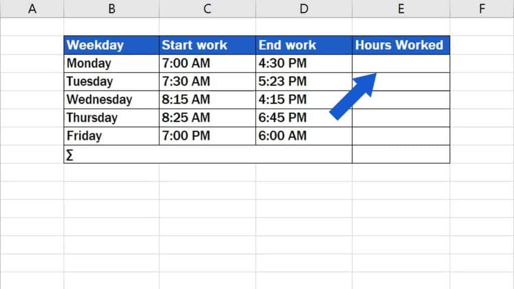
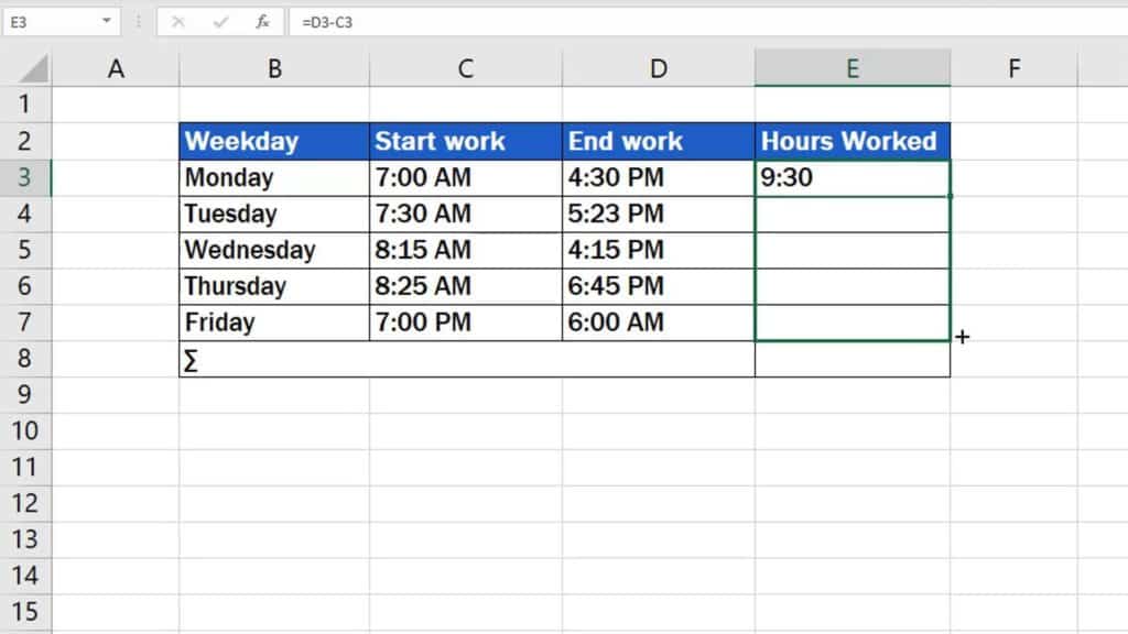
The table we prepared contains the time when an employee started and finished work. Hours worked can be calculated easily, as time difference – simply take the later time and subtract the earlier one.
Keep in mind one rule, though.
If Excel is to subtract time accurately and to display the right time format, cells must be formatted properly before the calculation takes place. Formatting of the cells in this table was set in the previous tutorial. If you want to know more about how to set the right formatting, watch our video on how to insert and format time in Excel.
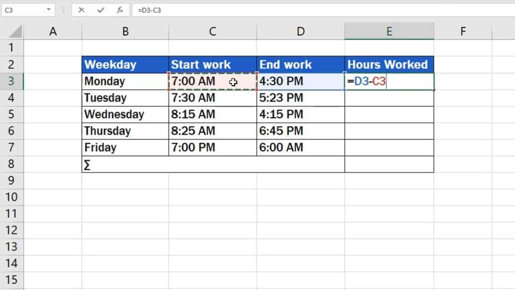
If the cells have been formatted as needed, click in the cell where you want the result to appear. In this case it’s cell E3.
Type in the ‘equal’ sign and click on the cell that contains the later time value, which means 4:30 PM here. Since we’re subtracting, insert the minus and now just add the time logged under ‘Start Work’.
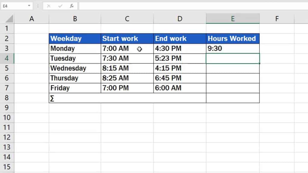
Press ‘Enter’, and we’ve got the result! On Monday, the employee worked nine hours and thirty minutes in total.
How to Calculate Hours Worked in Excel (whole week in a minute)
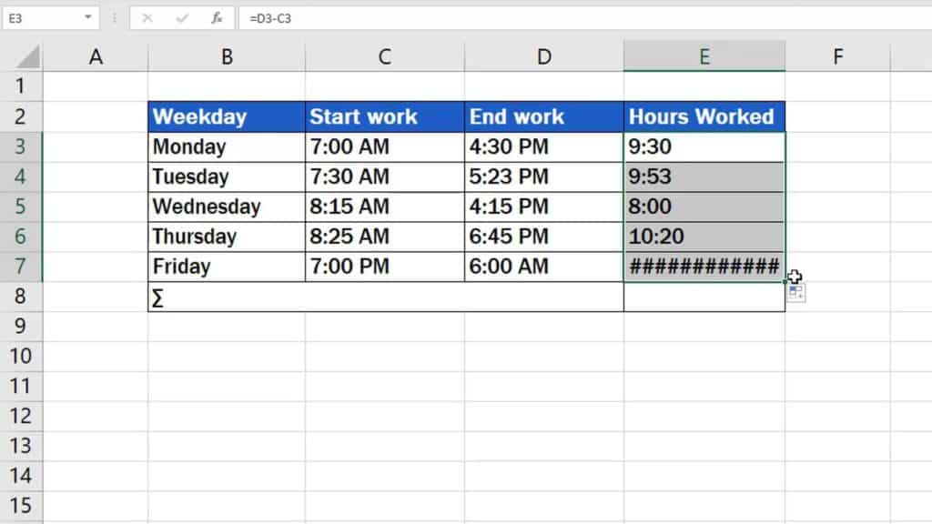
If you want to calculate hours worked for each day of the week, simply click on the bottom right corner of the cell containing the formula and drag down the cells where we need the formula to do the calculation, too.
That’s it! Good job!
Simple calculation of hours worked for each day of the week has been done!
But watch out for this!
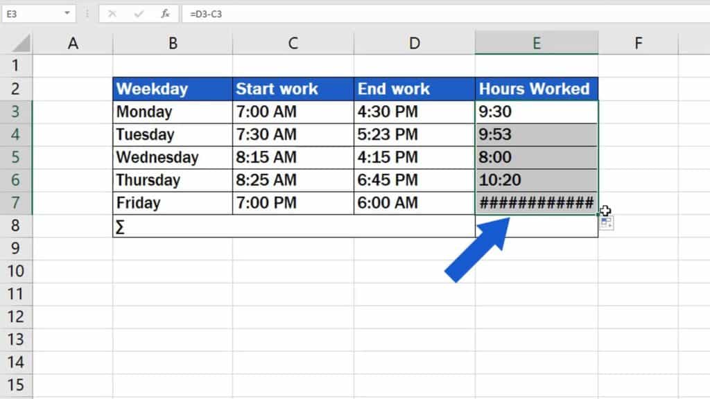
As you can see, the result for Friday displays only a set of hash signs. This is because the times when the employee started and finished work span midnight. The working time started at seven o’clock in the evening and ended the next morning at six.
To learn how to deal with such a situation, watch the next EasyClick Academy video tutorial on how to calculate time difference between two times that span midnight.
Don’t miss out a great opportunity to learn:
- How to Sum Time in Excel
- How to Calculate Hours Worked in Excel (Midnight Span)
- How to Insert and Format Time in Excel
If you’ve found this tutorial helpful, like us and subscribe to receive more videos from EasyClick Academy. Look at more tutorials that help you use Excel quick and easy!
See you in the next tutorial!
Chandoo posted an interesting challenge on his blog last Friday, challenging users to calculated hours worked for an employee name Billy. This example resonated with me for a couple of reasons. The first is that I’ve had to do this kind of stuff in the past, the second is because I’ve got a new toy I’d use to do it. (Yup… that toy would be Power Query.)
It always blows my mind how many people respond on Chandoo’s blog. As the answers were pouring in, I decided to tackle the issue my own way too. I thought I’d share a bit more detailed version of that here as I think many users still struggle with time in Excel.
Background and Excel Formula Solution
Chandoo provided a sample file on his blog, so I downloaded it. The basic table of data looks like this:

Now, for anyone who has done this a long time, there a few key pieces to solving this:
- The recognition that all times are fractions of days,
- The recognition that if you omit the day it defaults to 1900-01-01, and
- The data includes End times that are intended to be the day following the Start time
The tricks we use to deal with this are:
- Test if the End time is less than the start time. If so, add a day. (This allows us to subtract the Start from the End and get the difference in hours.
- Multiply the hours by 24. (This allows us to convert the fractional time into a number that represents hours instead of fractions of a day.)
Easy enough, and the following submitted formula (copied down from F4:F9 and summed) works:
=(D4+IF(C4>D4,1,0)-C4)*24

Also, there was a great comment that Billy shouldn’t get paid for his lunch break. Where I used to work (before I went out on my own), we had a rule that if you worked any more than 4 hours you MUST take a lunch break. Plumbing in that logic, we’d would need a different formula. There’s lots that would work, and this is one:
=((D4+IF(C4>D4,1,0)-C4)*24)-IF(((D4+IF(C4>D4,1,0)-C4)*24)>4,1,0)

So why Power Query?
If we can do this in Excel, why would we cook up a Power Query solution? Easy. Because I’m tired of having to actually write the formula every time Billy sends me his timesheet. Formula work is subject to error, so why not essentially automate the solution?
Using Power Query to Calculate Hours Worked
Okay, first thing I’m going to do is set up a system. I’m set up a template, email to Billy and get him to fill it out and email it to me every two weeks. I’ll save the file in a folder, and get to work.
- Open a blank workbook –> Power Query –> From File –> From Excel
- Browse and locate the file
- Select the “Billy” worksheet (Ok, to be fair, it would probably be called Sheet1 in my template)

- Click Edit
And now the fun begins…
- Home –> Remove Rows –> Remove Top Rows –> 2
- Transform –> Use First Row as Headers
- Filter the Day column to remove (null) values
- Select the Day:End columns –> right click –> Remove Other Columns
And we’ve now got a nice table of data to start with:

Not bad, but the data type for the Start and End columns is set to “any”. That’s bad news to me, as I want to do some Date/Time math. The secret here is that we need our values to be Date/Times (not just times), so let’s force that format on them, just to be safe:
- Select Start:End –> Transform –> Date/Time
Next, we need to test if the Start Date occurs after the End Date. Let’s use one step to test that and add one day if it’s true:
- Add Column –> Add Custom Column
- Name: Custom
- Formula: =if [Start]>[End] then Date.AddDays([End],1) else [End]
So basically, we add 1 day to the End data if the Start time is greater than the end time. Once we’ve done that, we can:
- Right click the End column –> Remove
- Right click the Custom column –> Rename –> End
And, as you can see, we’ve got 3 records that have been increased by a day (they are showing 12/31/1899 instead of 12/30/1899

Good stuff, let’s figure out the difference between these two. The order of the next 3 steps is important…
- Select the End column
- Hold down the CTRL key and select the Start column
- Go to Add Column –> Time –> Subtract
Because we selected the Start column second, it is subtracted from the End column we selected first:

Now we can set the Start and End columns so that only show times, as we don’t need the date portion any more. In addition, we want to convert the TimeDifference to hours:
- Select the Start:End columns –> Transform –> Time
- Select the TimeDifference column –> Transform –> Decimal Number
Hmm… that didn’t work quite as cleanly as we’d like:

Ah… but times are fractions of days, right? Let’s multiply this column by 24 and see what happens:
- With the TimeDifference column selected: Transform –> Standard –> Multiply –> 24
- Right click the TimeDifference column –> Rename –> Hours
Nice!

Oh… but what about those breaks?
- Add Column –> Add Custom Column
- Name: Breaks
- Formula: =if [Hours]>4 then -1 else 0
- Add Column –> Add Custom Column
- Name: Net Hours
- Formula: =[Hours]+[Breaks]
And here we go:

At this point I would generally:
- Change the name of the query to something like: Timesheet
- Close and Load to a Table
- Add a total row to the table

But just in case you only cared about the total of the Net Hours column, we could totally do that in Power Query as well. Even though it’s not something I would do (I’m sure Billy would trust YOU implicitly and never want to see the support that proved you added things up correctly…), here’s how you’d do it:
- Go to Transform –> Group By
- Click the – character next to the Day label to remove that grouping level
- Set up the Grouping column:
- Name: Net Hours
- Operation: Sum
- Column: Net Hours
Here’s what it looks like if you set the column details up first, indicating where to click to remove the grouping level:

And the result after you click OK:

Holy Cow that’s a LOT of Work!?!
Not really. Honestly, it took me about a minute to cook it up. (And a LOT longer to write this post.) But even better, this work was actually an investment. Next time I get a timesheet, I just save it over the old one, open this file, right click the table and click Refresh. Done, dusted, finished and time to move on to more challenging problems.
Even better, if I wanted to get really serious with it, I could implement a parameter function to make the file path relative to the file, and then I could pass it off to someone else to refresh. Or automate the refresh completely. After all, why write formulas every month if you don’t have to?
🙂
Timesheet in Excel Template (Table of Contents)
- Timesheet in Excel
- How to Create Timesheet Template in Excel?
Timesheet in Excel
Timesheet is a system for recording the number of employee’s time spent on each job. In excel, we normally use a timesheet to calculate the employee’s timings like IN and OUT timings, how many hours an employee worked for a day, what is the exact “BREAK” time he has taken. In excel, this timesheet will summarize the number of hours worked by each employee; in order to calculate these timings, we can use the timesheet to elaborate it.
How to Create Timesheet Template in Excel?
Creating a timesheet template in excel is very simple and easy. Let’s understand how to create a timesheet template in excel with some examples.
You can download this Timesheet Excel Template here – Timesheet Excel Template
Excel Timesheet – Example #1
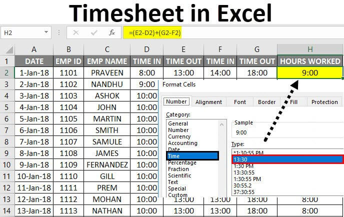
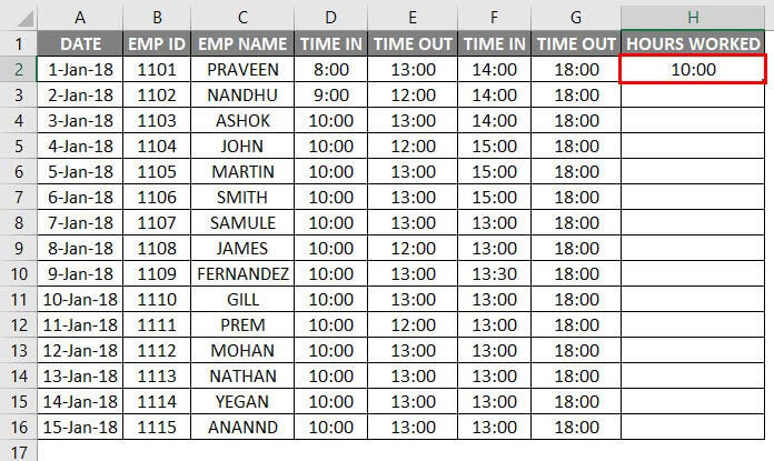
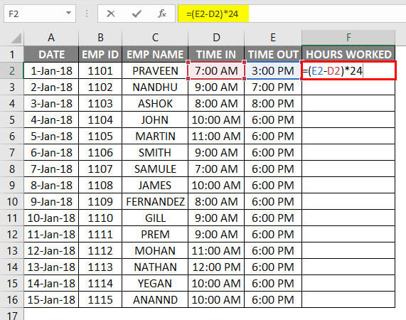
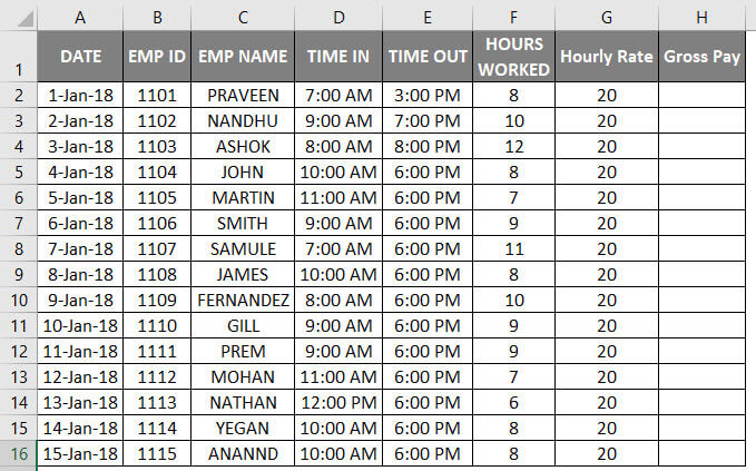
In this example, we are going to create a timesheet of employees by calculating how much hours an employee worked. First, let’s consider the below employee database with IN and OUT Timings.
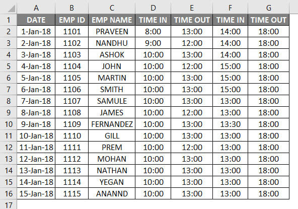
The above employee database has a date, employee name, TIME IN, and TIME OUT. Now we need to find out how much hours an employee worked by following the below steps:
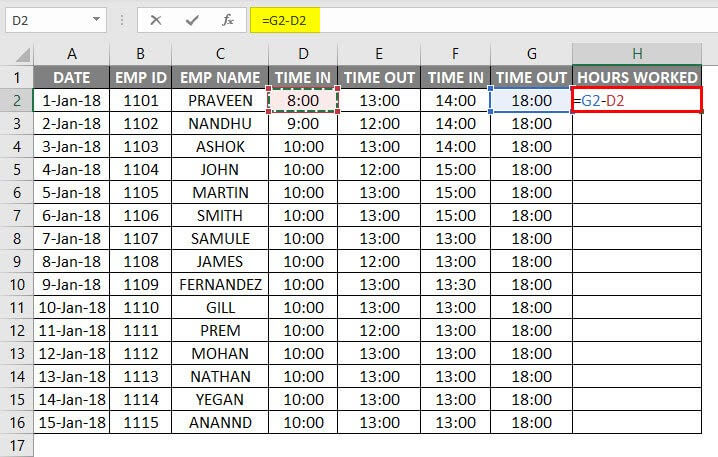
- First, create a new column named Number of Hours Worked.
- Make sure that the cell is in proper time format.
- In order to calculate an employee’s no of hours, we will calculate the formula as OUT TIMINGS – IN TIMINGS.
- By default, Excel will return the result in decimal numbers, as shown below, where it’s not an exact number of hours.
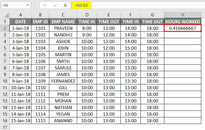
- We need to change this general format to time by formatting the cell, as shown below.
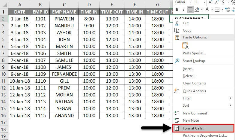
- Once we click on the format cell, we will get the below dialog box, choose the exact time format, and then click on ok.
- After applying the format, we will get the output result as follows.
- If we have IN and OUT Timings, we can use the formula as shown above, but we have BREAK TIME IN and TIME OUT in this example. Hence we can use the simple excel timesheet formula as =(E2-D2)+(G2-F2).
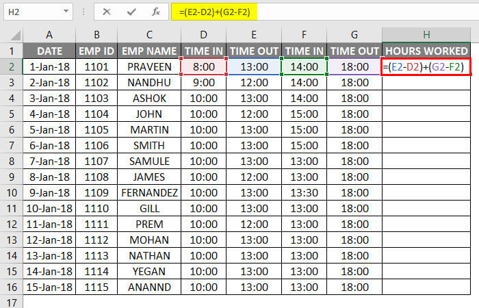
- By applying this formula, we will know how many hours an employee worked for a day, and the output will be displayed as follows.
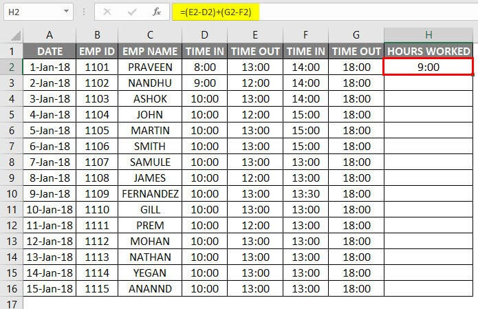
- We just need to drag the cell H2 downwards, and the formula will be applied for all the cells.
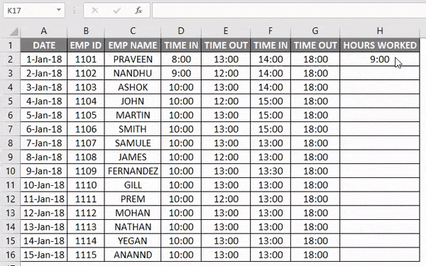
In the above example, we can see the time difference in how many hours an employee has worked and the breakup timings given for each employee as time OUT.
Excel Timesheet – Example #2
In the previous example, we have seen how many hours an employee has been worked using the normal arithmetic formula; now, in this example, we will use the time function in 24 hours format.
Suppose assume that management wants to pay the employees on an hourly basis based on their work timings.
Let’s consider the employee database with appropriate timings record, as shown below.
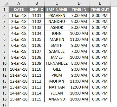
Here we can see that employee IN and OUT timings for various employees. Now we need to calculate the number of hours employee has been worked by following with the below steps:
- Insert new column named Hours Worked.
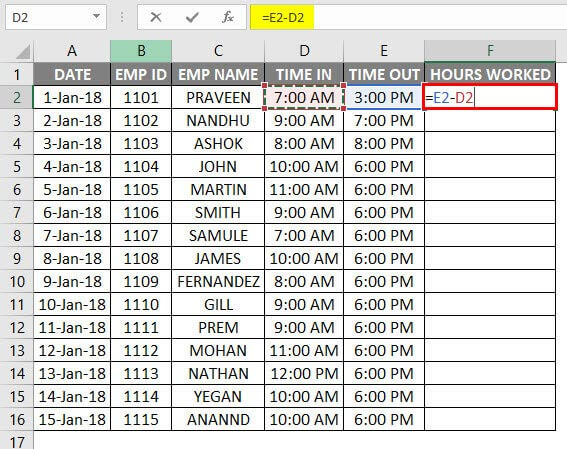
- Apply the normal excel timesheet formula as =E2-D2, as shown below.
- Now we can see that decimal values have been appeared for Hours Worked.
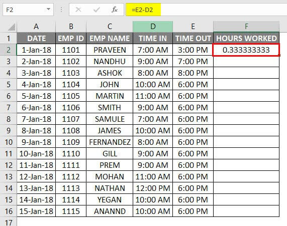
- This error normally occurs because the time is not in 24-hour format.
- To apply the excel timesheet formula by multiplying by 24 as =(E2-D2)*24.
- After applying the above formula, we will get the output result as follows.
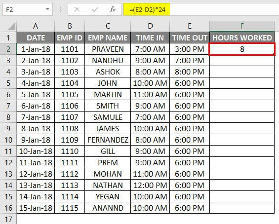
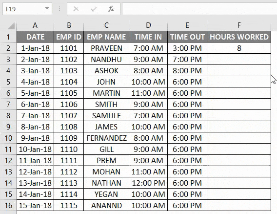
- Drag the cell F2 downwards, and the formula will be applied for all the cells, as shown below.
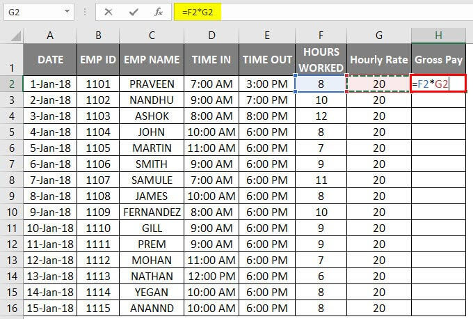
Now we will calculate how many employees are going to get paid on an hourly basis. Let’s assume that an employee will be paid for Rs.20/- per hour and follow the below steps.
- Insert two new columns as Hourly Rate and Gross Pay as given below.
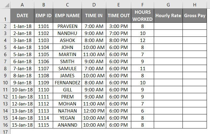
- In hourly Rate Column enter Rs.20/-.
- To apply the excel timesheet formula as Gross Pay = Hourly Rate * Hours Worked.
- We will get the below result as follows.
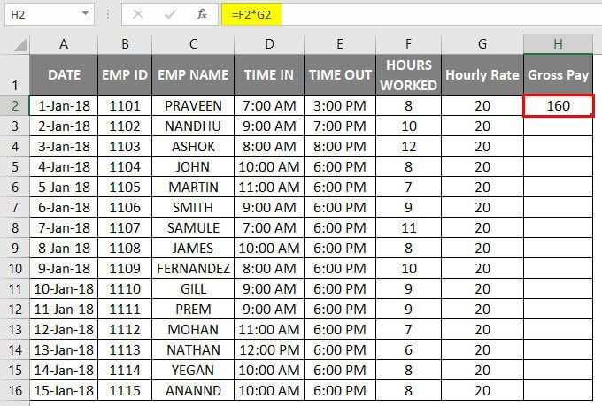
- Drag the cell H2 downwards, and the formula will be applied for all the cells, as shown below.
Here we calculated the Gross Pay of an employee based on the Number of Hours Worked.
Either way, we can create a new column Hourly Rate as Rs.20/- in a fixed column and multiply it by the Number of Hours Worked. Let’s see with an example as follows.
Excel Timesheet – Example #3
Consider the same employee data record, which has TIME IN and TIME OUT records.
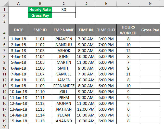
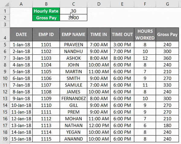
Here we have created a new fixed column named Hourly Rate as Rs.30/-. So employee will be get paid Rs.30/- Per Hour.
Now Hourly Rate has a fixed column, so whenever the Rate changes, it will get populated and reflected in the Gross Pay column as shown in the below steps.
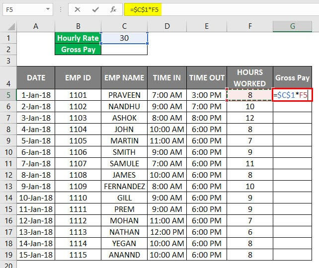
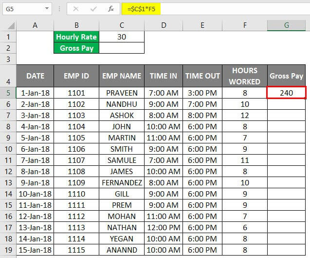
- Insert the excel timesheet formula in Gross Pay Column as =$c$1*F5 shown below, i.e. Gross Pay = Hourly Rate * Hours Worked.
- We can see that Gross Pay has been calculated as per the Hourly Rate Basis.
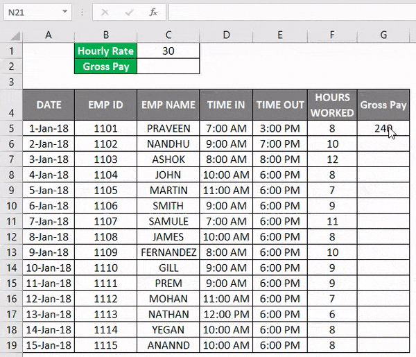
- Drag the cell G2 downwards, and the formula will be applied for all the cells, as shown below.
- Next, we will calculate the Total Gross Pay by adding the Gross Pay of the employees.
- Use the formula =SUM(G5:G19).
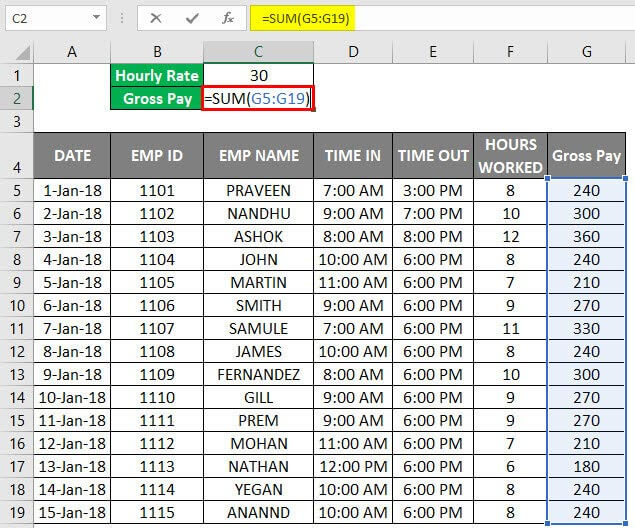
- We will get the below output as follows.
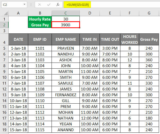
Hence we have calculated Total Gross Pay as Rs.3900/- and Hourly Rate as Rs.30/- If the Hours Rate changes, the values will be get automatically changed, and the same Gross Total also will be get changed.
Let’s see what happens if the Hourly Rate is changed to Rs.10/- and we will get the below result.
Now we can see the difference in each employee that Gross Pay has been getting decreased because of Changes in Hourly Rate and at the same time we got Total Gross Pay as Rs.1300/- and Hourly Rate as Rs.10/.
Things to Remember
- Maintain proper timing format while creating a timesheet for employees.
- Make sure that all cells are formatted in 24-hour format, or else excel will throw a decimal value.
- Ensure that AM and PM are mentioned in the timings because if the OUT TIME is Greater than IN TIME, excel will not be able to calculate the number of hours worked.
Recommended Articles
This has been a guide to Timesheet in Excel. Here we discuss how to create a Timesheet Template in Excel along with practical examples and a downloadable excel template. You may also look at the following articles to learn more –
- Time Function in Excel
- Worksheets in Excel
- VBA Worksheets
- Timecard Template in Excel
Microsoft Excel contains formatting tools and formulas to help you calculate the mixed time units of hours and minutes worked. Inserting a colon or “:” symbol between the hours and minutes will separate these two types of units prior to calculating. For example, to enter a two-hour task, type “2:00” with at least one digit to represent hours, and two digits to represent minutes after the colon. A custom format and the AutoSum command will calculate these mixed units. To differentiate the total hours worked from the addends, you can insert a cell border or a bold font to make the total value stand out on the worksheet. Microsoft also features templates, such as time sheets with formulas, to calculate the sums with each new time value entry (see the link in Resources).
Formatting Cells and AutoSum
Step 1
Open a new worksheet and enter the hours and minutes and a colon or “:” symbol inserted between these time units. For example, if an employee worked six hours and 45 minutes, enter “6:45” in a cell. If the duration is less than 60 minutes, enter “0:” for zero hours followed by the minutes. For example, enter “0:15” to indicate 15 minutes. To type full hours with no minutes, enter “:00” after the number of hours. For example, enter “3:00” for three full hours. Continue entering time values in contiguous cells in a row or column.
Step 2
Click in the cell where you want the total hours worked to calculate and display the sum. A rectangle will frame this empty cell.
Step 3
Click the “Home” tab and then click “Format” in the Cells group. Click “Format Cells” in the Protection section on the drop-down list.
Step 4
Click the «Number» tab and then click “Custom” in the Category list. Type “[h]:mm;@” (without the quotes) in the Type field. The two punctuation symbols surrounding the minutes or «mm» are the colon and semi-colon. Click “OK.” The cell will still be empty.
Step 5
Click “Σ AutoSum” in the Editing group. An animated dashed line will frame the addends. Press “Enter” to calculate and display the sum of hours and minutes worked.
Step 6
Enter “Total Hours” in the next cell to identify this value and then press “Enter.” To differentiate this cell containing the total value from the addends, you can opt to make the font bold by clicking the cell and then pressing “Ctrl-B”.
Step 7
Save this worksheet.
Templates
Step 1
Open Excel and enter “time sheet” in the Search Bar for Online Templates box. Press “Enter” to bring up the gallery of Excel thumbnail templates.
Step 2
Click the preferred thumbnail to enlarge and preview. Click or tap “Create” to open the template on a new Excel worksheet.
Step 3
Enter the employee’s data in the fields and the quantity of hours worked in the cells. For example, to type 7 hours and 45 minutes, enter “7.75” in the cell. The total hours will recalculate with each new value. If the template does not show the total value, click a cell where you want the total to display, and then click “Σ AutoSum” in the Editing group on the Home tab. Press “Enter” to display the sum.
Step 4
Save this worksheet.
References
Resources
Tips
- The custom format, [h]:mm;@, will save to the Type list for future use.
- To add a cell border around the total hours worked, click the cell and then click the “Borders” arrow button in the Font group on the Home tab. Click “Top and Double Bottom Border” on the drop-down list, for example. Press “Enter” to move the cursor to the next cell and display the cell border.
- To edit the template, click inside the worksheet to bring up the Table Tools ribbon and the Design tab. Click the «Design» tab to display a gallery of Table Styles that can help make your data look more visually interesting to your viewer.
Warnings
- Information in this article applies to Microsoft Excel 2013 Home and Business. It may vary slightly or significantly with other versions or products.
Image Credit
Ablestock.com/AbleStock.com/Getty Images