
Watch Video – 3 Ways to Create a Histogram Chart in Excel
A histogram is a common data analysis tool in the business world. It’s a column chart that shows the frequency of the occurrence of a variable in the specified range.
According to Investopedia, a Histogram is a graphical representation, similar to a bar chart in structure, that organizes a group of data points into user-specified ranges. The histogram condenses a data series into an easily interpreted visual by taking many data points and grouping them into logical ranges or bins.
A simple example of a histogram is the distribution of marks scored in a subject. You can easily create a histogram and see how many students scored less than 35, how many were between 35-50, how many between 50-60 and so on.
There are different ways you can create a histogram in Excel:
- If you’re using Excel 2016, there is an in-built histogram chart option that you can use.
- If you’re using Excel 2013, 2010 or prior versions (and even in Excel 2016), you can create a histogram using Data Analysis Toolpack or by using the FREQUENCY function (covered later in this tutorial)
Let’s see how to make a Histogram in Excel.
Creating a Histogram in Excel 2016
Excel 2016 got a new addition in the charts section where a histogram chart was added as an inbuilt chart.
In case you’re using Excel 2013 or prior versions, check out the next two sections (on creating histograms using Data Analysis Toopack or Frequency formula).
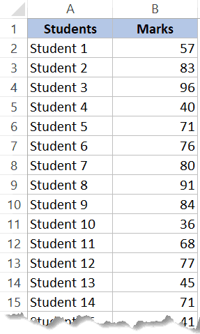
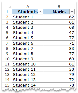
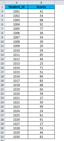
Suppose you have a dataset as shown below. It has the marks (out of 100) of 40 students in a subject.
Here are the steps to create a Histogram chart in Excel 2016:
- Select the entire dataset.
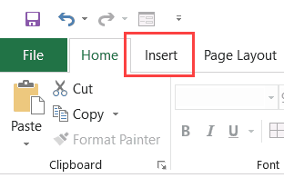
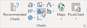
- Click the Insert tab.

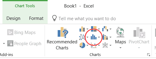
- In the Charts group, click on the ‘Insert Static Chart’ option.

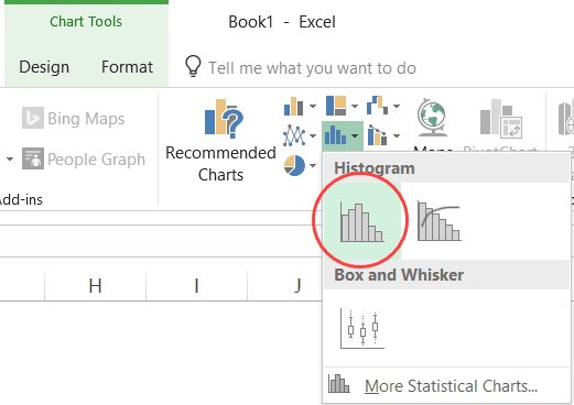
- In the HIstogram group, click on the Histogram chart icon.

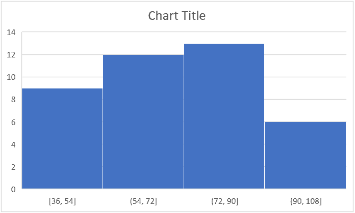
The above steps would insert a histogram chart based on your data set (as shown below).
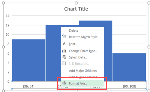
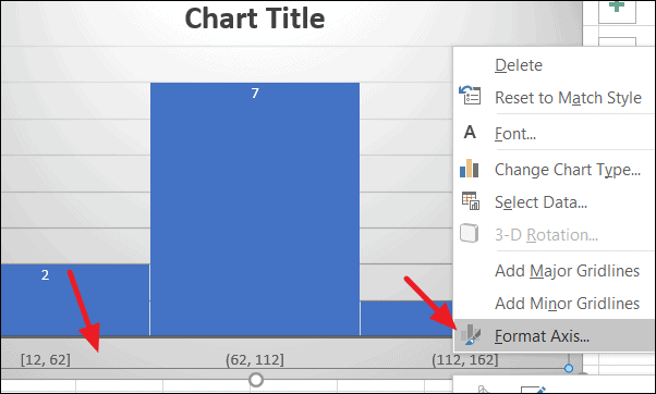
Now you can customize this chart by right-clicking on the vertical axis and selecting Format Axis.
This will open a pane on the right with all the relevant axis options.
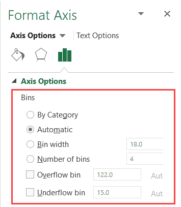
Here are some of the things you can do to customize this histogram chart:
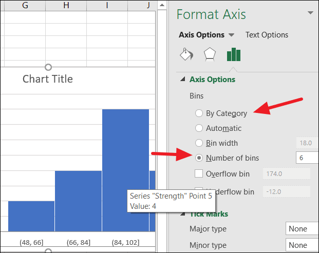
- By Category: This option is used when you have text categories. This could be useful when you have repetitions in categories and you want to know the sum or count of the categories. For example, if you have sales data for items such as Printer, Laptop, Mouse, and Scanner, and you want to know the total sales of each of these items, you can use the By Category option. It isn’t helpful in our example as all our categories are different (Student 1, Student 2, Student3, and so on.)
- Automatic: This option automatically decides what bins to create in the Histogram. For example, in our chart, it decided that there should be four bins. You can change this by using the ‘Bin Width/Number of Bins’ options (covered below).
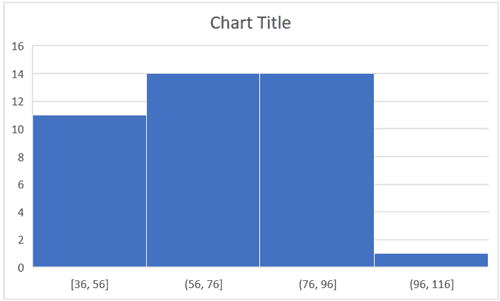
- Bin Width: Here you can define how big the bin should be. If I enter 20 here, it will create bins such as 36-56, 56-76, 76-96, 96-116.

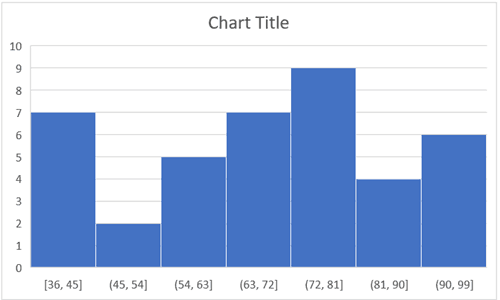
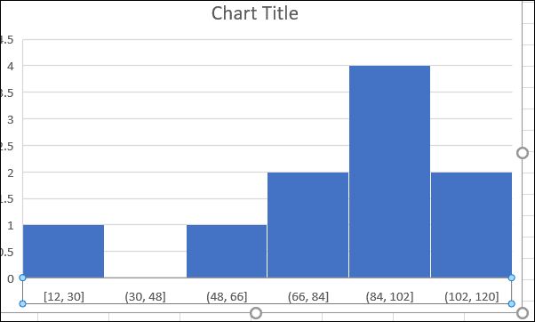
- Number of Bins: Here you can specify how many bins you want. It will automatically create a chart with that many bins. For example, if I specify 7 here, it will create a chart as shown below. At a given point, you can either specify Bin Width or Number of Bins (not both).

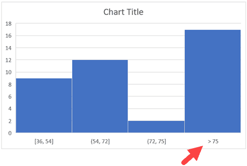
- Overflow Bin: Use this bin if you want all the values above a certain value clubbed together in the Histogram chart. For example, if I want to know the number of students that have scored more than 75, I can enter 75 as the Overflow Bin value. It will show me something as shown below.

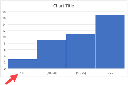
- Underflow Bin: Similar to Overflow Bin, if I want to know the number of students that have scored less than 40, I can enter 4o as the value and show a chart as shown below.

Once you have specified all the settings and have the histogram chart you want, you can further customize it (changing the title, removing gridlines, changing colors, etc.)
Creating a Histogram Using Data Analysis Tool pack
The method covered in this section will also work for all the versions of Excel (including 2016). However, if you’re using Excel 2016, I recommend you use the inbuilt histogram chart (as covered below)
To create a histogram using Data Analysis tool pack, you first need to install the Analysis Toolpak add-in.
This add-in enables you to quickly create the histogram by taking the data and data range (bins) as inputs.
Installing the Data Analysis Tool Pack
To install the Data Analysis Toolpak add-in:
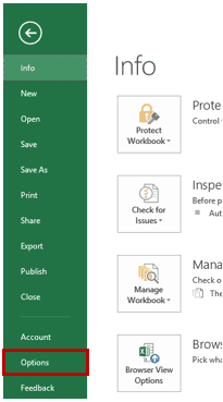
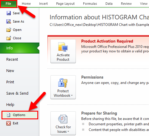
- Click the File tab and then select ‘Options’.
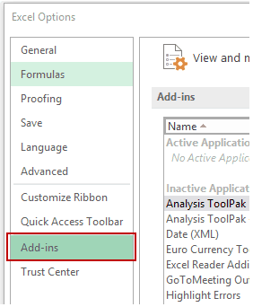
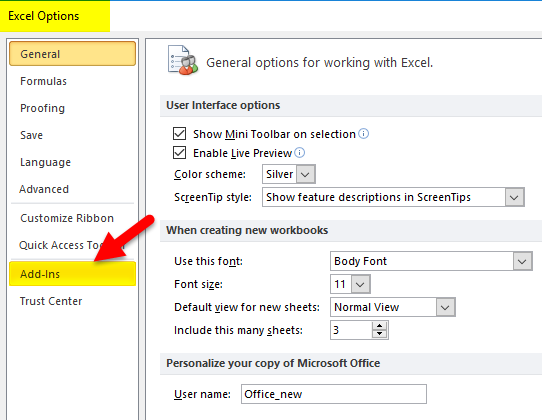
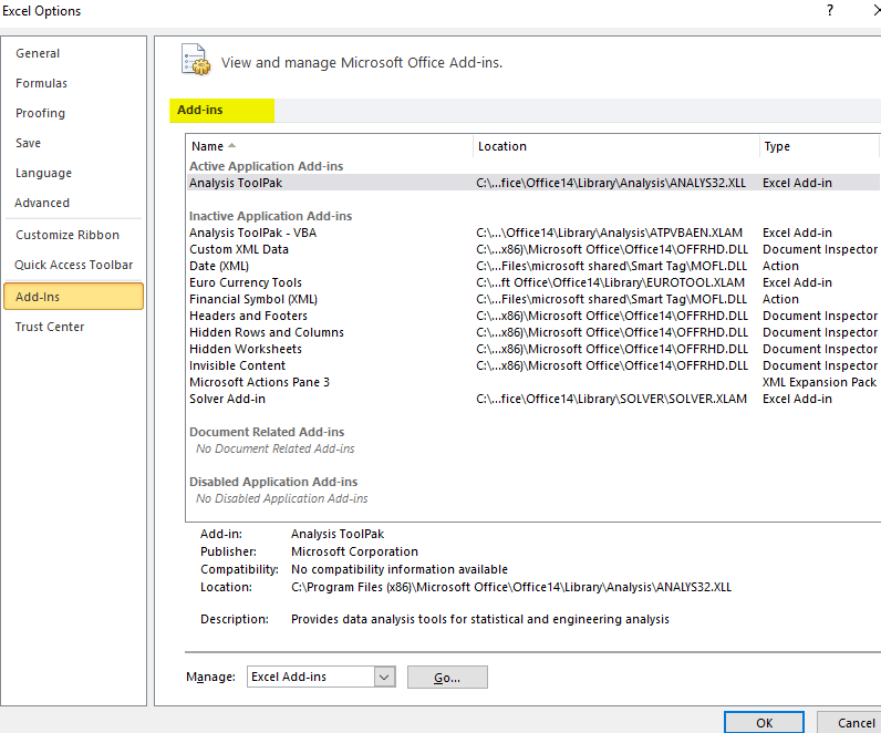
- In the Excel Options dialog box, select Add-ins in the navigation pane.
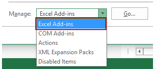
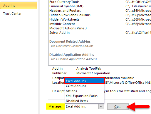
- In the Manage drop-down, select Excel Add-ins and click Go.
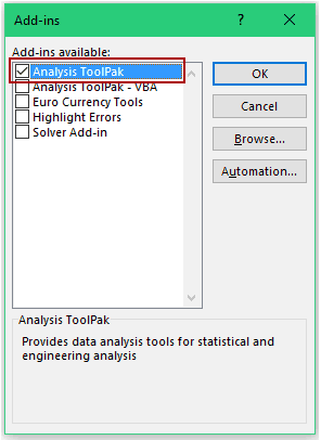
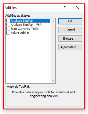
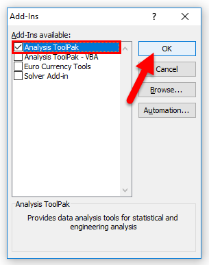
- In the Add-ins dialog box, select Analysis Toolpak and click OK.
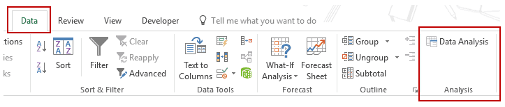
This would install the Analysis Toolpak and you can access it in the Data tab in the Analysis group.
Creating a Histogram using Data Analysis Toolpak
Once you have the Analysis Toolpak enabled, you can use it to create a histogram in Excel.
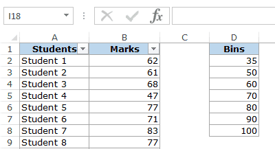
Suppose you have a dataset as shown below. It has the marks (out of 100) of 40 students in a subject.
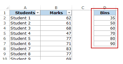
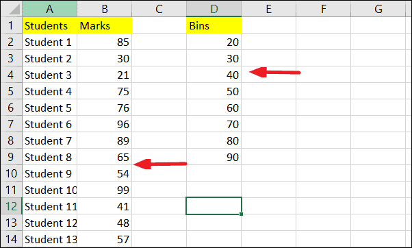
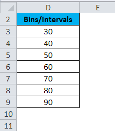
To create a histogram using this data, we need to create the data intervals in which we want to find the data frequency. These are called bins.
With the above dataset, the bins would be the marks intervals.
You need to specify these bins separately in an additional column as shown below:
Now that we have all the data in place, let’s see how to create a histogram using this data:
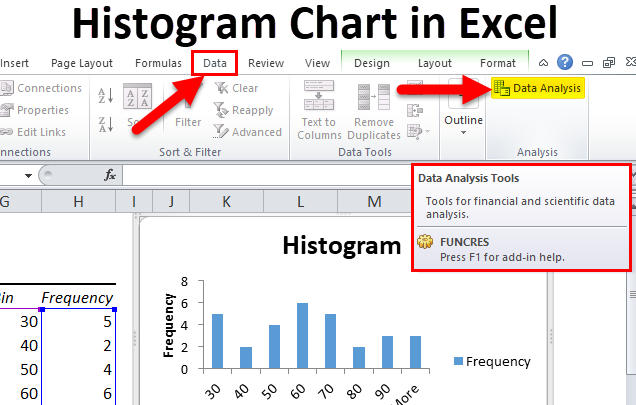
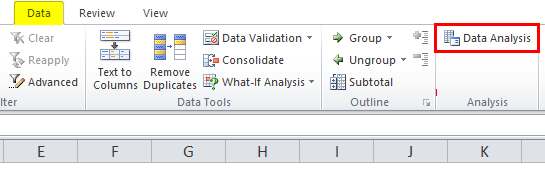
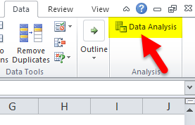
- Click the Data tab.
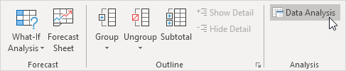
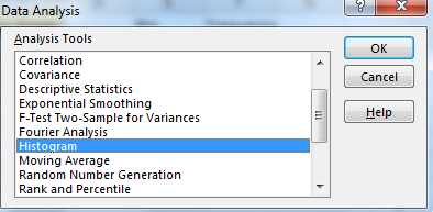
- In the Analysis group, click on Data Analysis.
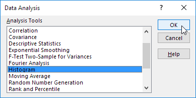
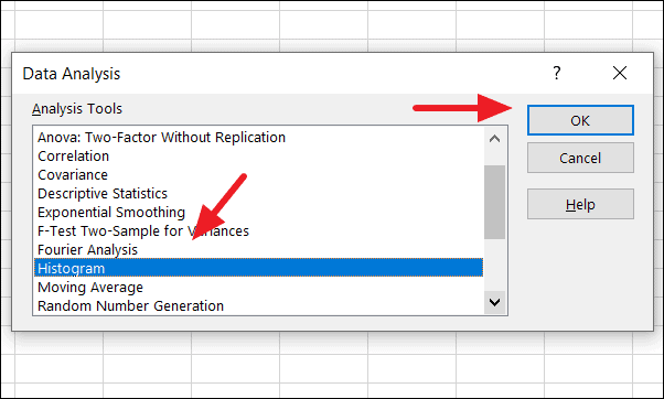
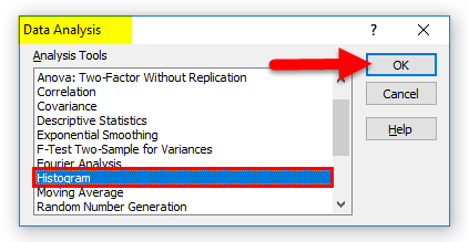
- In the ‘Data Analysis’ dialog box, select Histogram from the list.
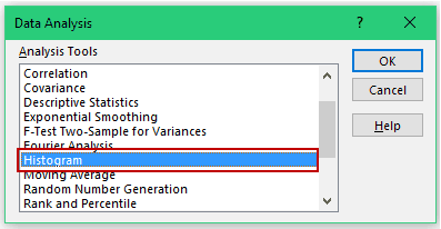
- Click OK.
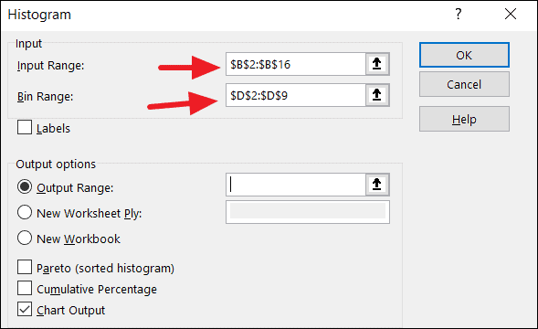
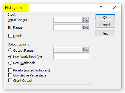
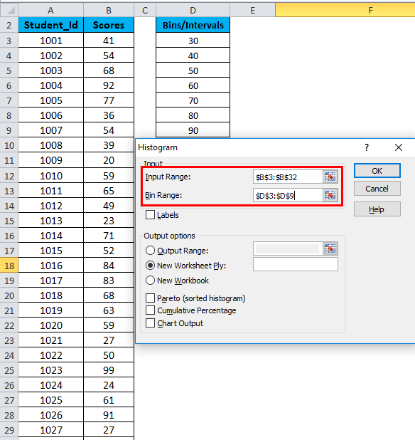
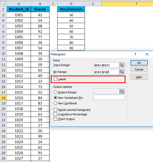
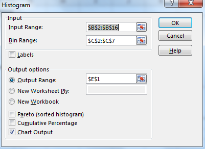
- In the Histogram dialog box:
- Select the Input Range (all the marks in our example)
- Select the Bin Range (cells D2:D7)
- Leave the Labels checkbox unchecked (you need to check it if you included labels in the data selection).
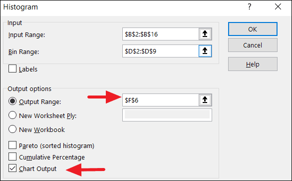
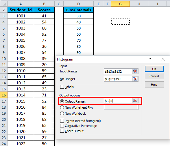
- Specify the Output Range if you want to get the Histogram in the same worksheet. Else, choose New Worksheet/Workbook option to get it in a separate worksheet/workbook.
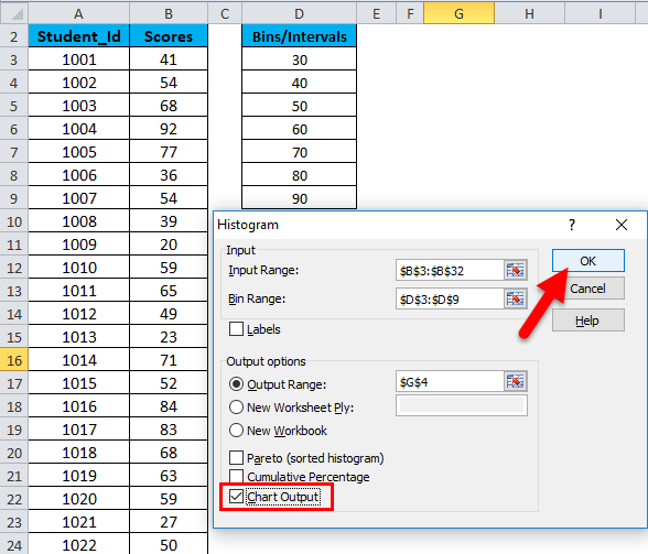
- Select Chart Output.
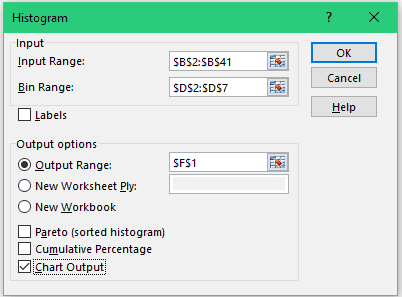
- Click OK.
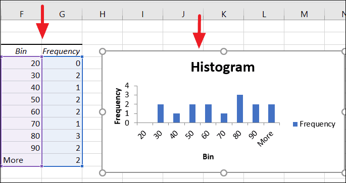
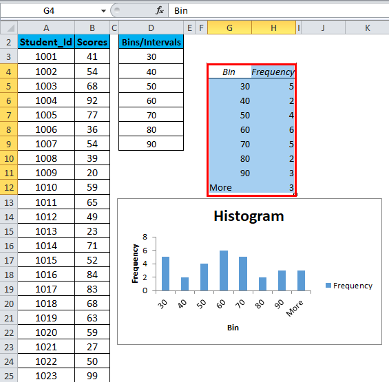
This would insert the frequency distribution table and the chart in the specified location.
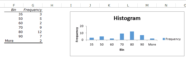
Now there are some things you need to know about the histogram created using the Analysis Toolpak:
- The first bin includes all the values below it. In this case, 35 shows 3 values indicating that there are three students who scored less than 35.
- The last specified bin is 90, however, Excel automatically adds another bin – More. This bin would include any data point which lies after the last specified bin. In this example, it means that there are 2 students who have scored more than 90.
- Note that even if I add the last bin as 100, this additional bin would still be created.
- This creates a static histogram chart. Since Excel creates and pastes the frequency distribution as values, the chart would not update when you change the underlying data. To refresh it, you’ll have to create the histogram again.
- The default chart is not always in the best format. You can change the formatting like any other regular chart.
- Once created, you can not use Control + Z to revert it. You’ll have to manually delete the table and the chart.
If you create a histogram without specifying the bins (i.e., you leave the Bin Range empty), it would still create the histogram. It would automatically create six equally spaced bins and used this data to create the histogram.
Creating a Histogram using FREQUENCY Function
If you want to create a histogram that is dynamic (i.e., updates when you change the data), you need to resort to formulas.
In this section, you’ll learn how to use the FREQUENCY function to create a dynamic histogram in Excel.
Again, taking the student’s marks data, you need to create the data intervals (bins) in which you want to show the frequency.
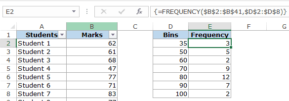
Here is the function that will calculate the frequency for each interval:
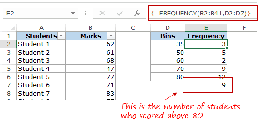
=FREQUENCY(B2:B41,D2:D8)
Since this is an array formula, you need to use Control + Shift + Enter, instead of just Enter.
Here are the steps to make sure you get the correct result:
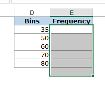
- Select all cells adjacent to the bins. In this case, these are E2:E8.
- Press F2 to get into the edit mode for cell E2.
- Enter the frequency formula: =FREQUENCY(B2:B41,D2:D8)
- Hit Control + Shift + Enter.
With the result that you get, you can now create a histogram (which is nothing but a simple column chart).
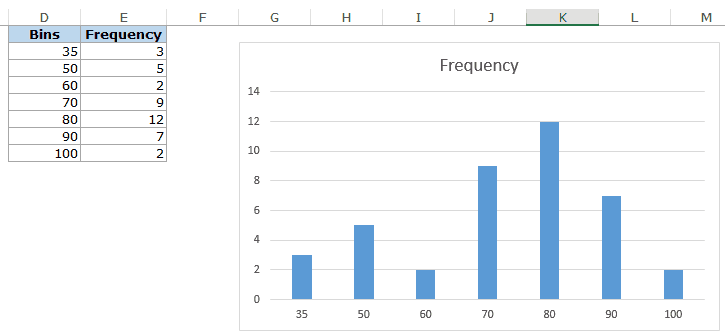
Here are some important things you need to know when using the FREQUENCY function:
- The result is an array and you can not delete a part of the array. If you need to, delete all the cells that have the frequency function.
- When a bin is 35, the frequency function would return a result that includes 35. So 35 means score up to 35, and 50 would mean score more than 35 and up to 50.
Also, let’s say you want to have the specified data intervals till 80, and you want to group all the result above 80 together, you can do that using the FREQUENCY function. In that case, select one more cell than the number of bins. For example, if you have 5 bins, then select 6 cells as shown below:
FREQUENCY function would automatically calculate all the values above 80 and return the count.
You May Also Like the Following Excel Tutorials:
- Creating a Pareto Chart in Excel.
- Creating a Gantt Chart in Excel.
- Creating a Milestone Chart in Excel.
- How to Make a Bell Curve in Excel.
- How to Create a Bullet Chart in Excel.
- How to Create a Heat Map in Excel.
- Standard Deviation in Excel.
- Area Chart in Excel.
- Advanced Excel Charts.
- Creating Excel Dashboards.
Excel 2013
-
Make sure you load the Analysis ToolPakto add the Data Analysis command to the Data tab.
-
On a worksheet, type the input data in one column, and the bin numbers in ascending order in another column.
-
Click Data > Data Analysis > Histogram > OK.
-
Under Input, select the input range (your data), then select the bin range.
-
Under Output options, choose an output location.
-
To show the data in descending order of frequency, click Pareto (sorted histogram).
-
To show cumulative percentages and add a cumulative percentage line, click Cumulative Percentage.
-
To show an embedded histogram chart, click Chart Output.
-
For more information, see Create a histogram.
Excel 2016
-
Select your data.
-
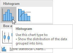
On the Insert tab, click Insert Statistic Chart > Histogram.

-
For more information, see Create a histogram.

Need more help?
Want more options?
Explore subscription benefits, browse training courses, learn how to secure your device, and more.
Communities help you ask and answer questions, give feedback, and hear from experts with rich knowledge.
Содержание
- Histogram
- How to Make a Histogram in Excel (Step-by-Step Guide)
- Creating a Histogram in Excel 2016
- Creating a Histogram Using Data Analysis Tool pack
- Installing the Data Analysis Tool Pack
- Creating a Histogram using Data Analysis Toolpak
- Creating a Histogram using FREQUENCY Function
Histogram
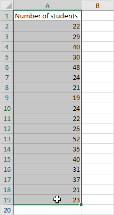
This example teaches you how to make a histogram in Excel.
1. First, enter the bin numbers (upper levels) in the range C4:C8.
2. On the Data tab, in the Analysis group, click Data Analysis.
Note: can’t find the Data Analysis button? Click here to load the Analysis ToolPak add-in.
3. Select Histogram and click OK.
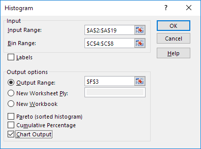
4. Select the range A2:A19.
5. Click in the Bin Range box and select the range C4:C8.
6. Click the Output Range option button, click in the Output Range box and select cell F3.
7. Check Chart Output.

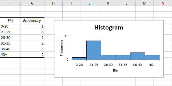
9. Click the legend on the right side and press Delete.
10. Properly label your bins.
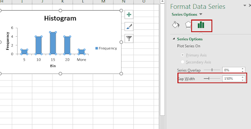
11. To remove the space between the bars, right click a bar, click Format Data Series and change the Gap Width to 0%.
12. To add borders, right click a bar, click Format Data Series, click the Fill & Line icon, click Border and select a color.
If you have Excel 2016 or later, simply use the Histogram chart type.
13. Select the range A1:A19.
14. On the Insert tab, in the Charts group, click the Histogram symbol.
15. Click Histogram.
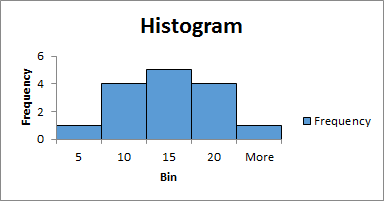
Result. A histogram with 3 bins.
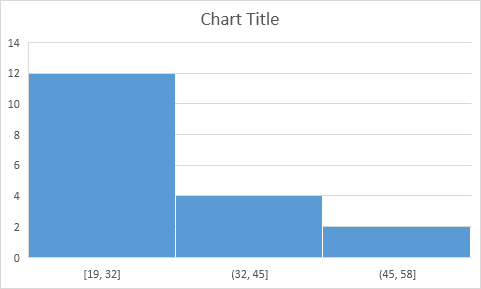
Note: Excel uses Scott’s normal reference rule for calculating the number of bins and the bin width.
16. Right click the horizontal axis, and then click Format Axis.
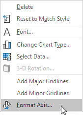
The Format Axis pane appears.
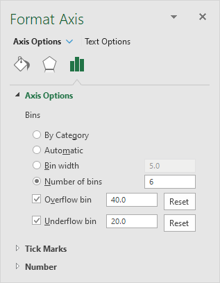
17. Define the histogram bins. We’ll use the same bin numbers as before (see first picture on this page). Bin width: 5. Number of bins: 6. Overflow bin: 40. Underflow bin: 20.
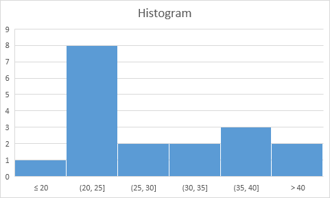
Recall, we made the following histogram using the Analysis ToolPak (steps 1-12).
Conclusion: the bin labels look different, but the histograms are the same. ≤20 is the same as 0-20, (20, 25] is the same as 21-25, etc.
Tip: you can also use pivot tables to easily create a frequency distribution in Excel.
Источник
How to Make a Histogram in Excel (Step-by-Step Guide)
Watch Video – 3 Ways to Create a Histogram Chart in Excel
A histogram is a common data analysis tool in the business world. It’s a column chart that shows the frequency of the occurrence of a variable in the specified range.
According to Investopedia, a Histogram is a graphical representation, similar to a bar chart in structure, that organizes a group of data points into user-specified ranges. The histogram condenses a data series into an easily interpreted visual by taking many data points and grouping them into logical ranges or bins.
A simple example of a histogram is the distribution of marks scored in a subject. You can easily create a histogram and see how many students scored less than 35, how many were between 35-50, how many between 50-60 and so on.
There are different ways you can create a histogram in Excel:
- If you’re using Excel 2016, there is an in-built histogram chart option that you can use.
- If you’re using Excel 2013, 2010 or prior versions (and even in Excel 2016), you can create a histogram using Data Analysis Toolpack or by using the FREQUENCY function (covered later in this tutorial)
Let’s see how to make a Histogram in Excel.
This Tutorial Covers:
Creating a Histogram in Excel 2016
Excel 2016 got a new addition in the charts section where a histogram chart was added as an inbuilt chart.
In case you’re using Excel 2013 or prior versions, check out the next two sections (on creating histograms using Data Analysis Toopack or Frequency formula).
Suppose you have a dataset as shown below. It has the marks (out of 100) of 40 students in a subject.
Here are the steps to create a Histogram chart in Excel 2016:
- Select the entire dataset.
- Click the Insert tab.
- In the Charts group, click on the ‘Insert Static Chart’ option.
- In the HIstogram group, click on the Histogram chart icon.
The above steps would insert a histogram chart based on your data set (as shown below).
Now you can customize this chart by right-clicking on the vertical axis and selecting Format Axis.
This will open a pane on the right with all the relevant axis options.
Here are some of the things you can do to customize this histogram chart:
- By Category: This option is used when you have text categories. This could be useful when you have repetitions in categories and you want to know the sum or count of the categories. For example, if you have sales data for items such as Printer, Laptop, Mouse, and Scanner, and you want to know the total sales of each of these items, you can use the By Category option. It isn’t helpful in our example as all our categories are different (Student 1, Student 2, Student3, and so on.)
- Automatic: This option automatically decides what bins to create in the Histogram. For example, in our chart, it decided that there should be four bins. You can change this by using the ‘Bin Width/Number of Bins’ options (covered below).
- Bin Width: Here you can define how big the bin should be. If I enter 20 here, it will create bins such as 36-56, 56-76, 76-96, 96-116.
- Number of Bins: Here you can specify how many bins you want. It will automatically create a chart with that many bins. For example, if I specify 7 here, it will create a chart as shown below. At a given point, you can either specify Bin Width or Number of Bins (not both).
- Overflow Bin: Use this bin if you want all the values above a certain value clubbed together in the Histogram chart. For example, if I want to know the number of students that have scored more than 75, I can enter 75 as the Overflow Bin value. It will show me something as shown below.
- Underflow Bin: Similar to Overflow Bin, if I want to know the number of students that have scored less than 40, I can enter 4o as the value and show a chart as shown below.
Once you have specified all the settings and have the histogram chart you want, you can further customize it (changing the title, removing gridlines, changing colors, etc.)
Creating a Histogram Using Data Analysis Tool pack
The method covered in this section will also work for all the versions of Excel (including 2016). However, if you’re using Excel 2016, I recommend you use the inbuilt histogram chart (as covered below)
To create a histogram using Data Analysis tool pack, you first need to install the Analysis Toolpak add-in.
This add-in enables you to quickly create the histogram by taking the data and data range (bins) as inputs.
Installing the Data Analysis Tool Pack
To install the Data Analysis Toolpak add-in:
- Click the File tab and then select ‘Options’.
- In the Excel Options dialog box, select Add-ins in the navigation pane.
- In the Manage drop-down, select Excel Add-ins and click Go.
- In the Add-ins dialog box, select Analysis Toolpak and click OK.
This would install the Analysis Toolpak and you can access it in the Data tab in the Analysis group.
Creating a Histogram using Data Analysis Toolpak
Once you have the Analysis Toolpak enabled, you can use it to create a histogram in Excel.
Suppose you have a dataset as shown below. It has the marks (out of 100) of 40 students in a subject.
To create a histogram using this data, we need to create the data intervals in which we want to find the data frequency. These are called bins.
With the above dataset, the bins would be the marks intervals.
You need to specify these bins separately in an additional column as shown below:
Now that we have all the data in place, let’s see how to create a histogram using this data:
- Click the Data tab.
- In the Analysis group, click on Data Analysis.
- In the ‘Data Analysis’ dialog box, select Histogram from the list.
- Click OK.
- In the Histogram dialog box:
- Select the Input Range (all the marks in our example)
- Select the Bin Range (cells D2:D7)
- Leave the Labels checkbox unchecked (you need to check it if you included labels in the data selection).
- Specify the Output Range if you want to get the Histogram in the same worksheet. Else, choose New Worksheet/Workbook option to get it in a separate worksheet/workbook.
- Select Chart Output.
This would insert the frequency distribution table and the chart in the specified location.
Now there are some things you need to know about the histogram created using the Analysis Toolpak:
- The first bin includes all the values below it. In this case, 35 shows 3 values indicating that there are three students who scored less than 35.
- The last specified bin is 90, however, Excel automatically adds another bin – More. This bin would include any data point which lies after the last specified bin. In this example, it means that there are 2 students who have scored more than 90.
- Note that even if I add the last bin as 100, this additional bin would still be created.
- This creates a static histogram chart. Since Excel creates and pastes the frequency distribution as values, the chart would not update when you change the underlying data. To refresh it, you’ll have to create the histogram again.
- The default chart is not always in the best format. You can change the formatting like any other regular chart.
- Once created, you can not use Control + Z to revert it. You’ll have to manually delete the table and the chart.
If you create a histogram without specifying the bins (i.e., you leave the Bin Range empty), it would still create the histogram. It would automatically create six equally spaced bins and used this data to create the histogram.
Creating a Histogram using FREQUENCY Function
If you want to create a histogram that is dynamic (i.e., updates when you change the data), you need to resort to formulas.
In this section, you’ll learn how to use the FREQUENCY function to create a dynamic histogram in Excel.
Again, taking the student’s marks data, you need to create the data intervals (bins) in which you want to show the frequency.
Here is the function that will calculate the frequency for each interval:
Since this is an array formula, you need to use Control + Shift + Enter, instead of just Enter.
Here are the steps to make sure you get the correct result:
- Select all cells adjacent to the bins. In this case, these are E2:E8.
- Press F2 to get into the edit mode for cell E2.
- Enter the frequency formula: =FREQUENCY(B2:B41,D2:D8)
- Hit Control + Shift + Enter.
With the result that you get, you can now create a histogram (which is nothing but a simple column chart).
Here are some important things you need to know when using the FREQUENCY function:
- The result is an array and you can not delete a part of the array. If you need to, delete all the cells that have the frequency function.
- When a bin is 35, the frequency function would return a result that includes 35. So 35 means score up to 35, and 50 would mean score more than 35 and up to 50.
Also, let’s say you want to have the specified data intervals till 80, and you want to group all the result above 80 together, you can do that using the FREQUENCY function. In that case, select one more cell than the number of bins. For example, if you have 5 bins, then select 6 cells as shown below:
FREQUENCY function would automatically calculate all the values above 80 and return the count.
You May Also Like the Following Excel Tutorials:
Источник
This example teaches you how to make a histogram in Excel.
1. First, enter the bin numbers (upper levels) in the range C4:C8.
2. On the Data tab, in the Analysis group, click Data Analysis.
Note: can’t find the Data Analysis button? Click here to load the Analysis ToolPak add-in.
3. Select Histogram and click OK.
4. Select the range A2:A19.
5. Click in the Bin Range box and select the range C4:C8.
6. Click the Output Range option button, click in the Output Range box and select cell F3.
7. Check Chart Output.
8. Click OK.
9. Click the legend on the right side and press Delete.
10. Properly label your bins.
11. To remove the space between the bars, right click a bar, click Format Data Series and change the Gap Width to 0%.
12. To add borders, right click a bar, click Format Data Series, click the Fill & Line icon, click Border and select a color.
Result:
If you have Excel 2016 or later, simply use the Histogram chart type.
13. Select the range A1:A19.
14. On the Insert tab, in the Charts group, click the Histogram symbol.
15. Click Histogram.
Result. A histogram with 3 bins.
Note: Excel uses Scott’s normal reference rule for calculating the number of bins and the bin width.
16. Right click the horizontal axis, and then click Format Axis.
The Format Axis pane appears.
17. Define the histogram bins. We’ll use the same bin numbers as before (see first picture on this page). Bin width: 5. Number of bins: 6. Overflow bin: 40. Underflow bin: 20.
Result:
Recall, we made the following histogram using the Analysis ToolPak (steps 1-12).
Conclusion: the bin labels look different, but the histograms are the same. ≤20 is the same as 0-20, (20, 25] is the same as 21-25, etc.
Tip: you can also use pivot tables to easily create a frequency distribution in Excel.
A histogram is a graphical chart that shows the frequency distribution of discrete or continuous data. Histograms may look very similar to vertical bar graphs but they’re different. However, Histograms are used to show distributions of data while bar charts are used to compare data. A histogram, unlike a bar chart, shows no gaps between the bars.
A histogram chart in Excel is primarily used for plotting the frequency distribution of a data set. In Excel, you can create a histogram using the Data Analysis ToolPak or using a built-in histogram chart. Now, let’s see how to create a Histogram in Excel.
Installing the Data Analysis Tool Pack
The Histogram tool is not available in Excel by default. To access it, you need to install Analysis ToolPak Add-in on Excel. Once the Add-in is installed, the Histogram will be made available in the list of Analysis Tools or in the charts group.
To install Analysis ToolPak Add-in, open the ‘File’ menu in Excel.
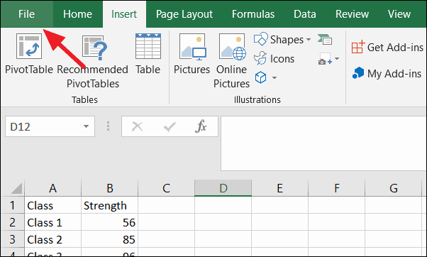
In the Excel backstage view, click ‘Options’.
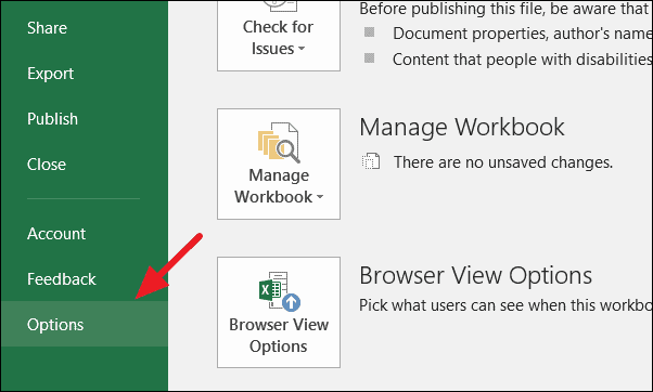
In ‘Excel Options’, Click on the ‘Add-ins’ tab on the left side.
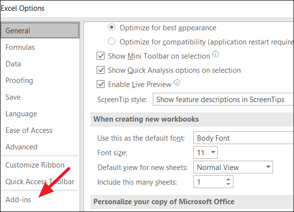
Here, you can view and manage your Microsoft Excel Add-ins. Select ‘Excel Add-in’ from the ‘Manage:’ drop-down at the bottom of the window and click ‘Go’.
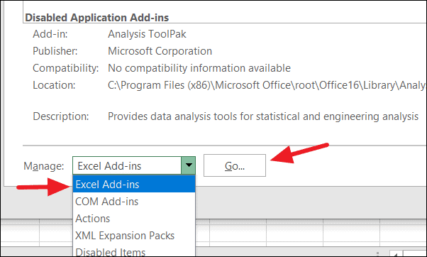
Then, check ‘Analysis ToolPak’ checkbox in the Add-ins dialog box and click ‘OK’.
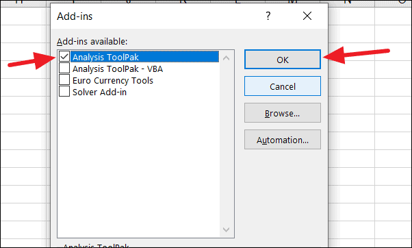
Now, the histogram tool is available in Excel, let’s see how to create one.
Creating a Histogram using Charts
First, create a dataset and select the range of cells containing the data to be displayed as histogram.
For example, let’s create a dataset for a number of students in 10 classes as shown below:
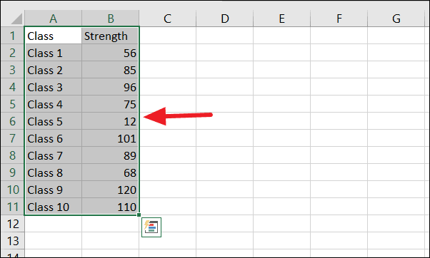
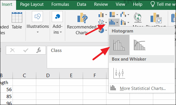
Select the range of cells and go to the ‘Insert’ tab. The histogram chart type is now available in the ‘Charts’ group of the Insert tab.
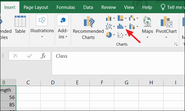
Click on the histogram icon and select your histogram chart type.
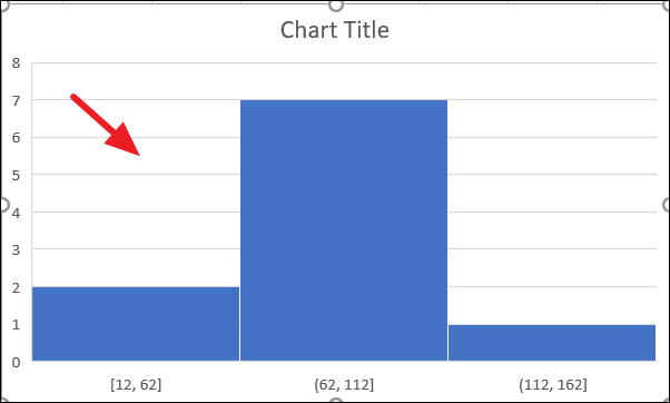
This would create a histogram with the distribution of data (marks) clubbed into bins as shown below.
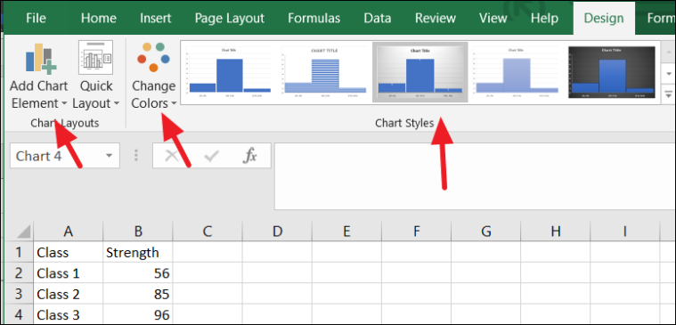
Once you created the histogram, you can customize it to fit your need in the ‘Design’ tab of Excel. You can add chart elements, change the colors of the bars, change chart styles, and switch rows and columns.
To format the X-Axis and Y-axis of the chart, right-click anywhere on the axis and select ‘Format Axis’ from the context menu.
This will open a format pane on the right-hand side of your Excel window. Here, you can further customize your axis to fit your need. You can change bin width, bin grouping, number of bins on the chart, etc.
For example, when we created the chart, Excel automatically made data into three-bin groupings. If we change the number of bins to 6, the data will be grouped into 6 bins.
The result is shown in the following picture.
Creating Histogram using Data Analysis Tool
Another way to make a histogram is by using Excel’s add-in program called Data Analysis toolpak. For creating a histogram, first, we need to create a data set and then data intervals (bins) at which we want to find the data frequency.
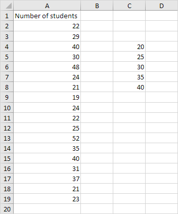
In the following example, column A and B contain the data set, and column D contains bins or mark intervals. We need to specify these bins separately.
Then, go to the ‘Data’ tab and click ‘Data Analysis’ in the Excel Ribbon.
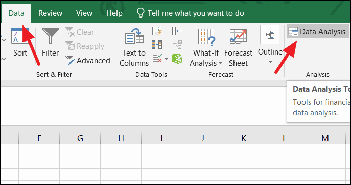
In the Data Analysis dialog box, select ‘Histogram’ from the list and click ‘OK’.
A Histogram dialog box will appear. In the Histogram dialog window, you need to specify the Input range, Bin range, and Output range.
Click on the ‘Input range’ box and select the range B2:B16 (which contains Marks). Then, click on the ‘Bin Range’ box and select the range D2:D9 (which contains data intervals).
Click the Output Range box and select a cell where you want the frequency distribution table to appear. Then, check ‘Chart Output’ and click ‘OK’.
Now, a Frequency Distribution table is created in the specified cell address along with the Histogram chart.
You can further improve the histogram by replacing the default Bins and Frequency with more relevant axis titles, changing chart style, customizing the chart legend, etc. Also, you can do the formatting of this chart like any other chart.
That’s it. Now, you know how to make a histogram in Excel.
Histogram chart (Table of Contents)
- Histogram in Excel
- Why is the histogram chart important in excel?
- Types/Shapes of the Histogram chart
- Where is the Histogram chart found?
- How to Create a Histogram Chart in Excel?
Histogram in Excel
Histogram Chart in excel is a data analysis tool used to show the periodic rise and drop in the data with the help of vertical columns. We can find the Histogram chart option if we are using Excel 2016, but for the older version MS Excel such as 2013 and 2010, we need to find this option in the Data Analysis option, which is available under the Data Analysis option.
Uses of Histogram Chart in Excel
A histogram is a graphical representation of the distribution of numerical data. A histogram is a column chart that shows the frequency of data in a certain range in a simpler way. It provides the visualization of numerical data by using the number of data points that fall within a specified range of values (also called “bins”).
A histogram chart in excel is classified or made up of 5 parts:
- Title: The title describes the information about the histogram.
- X-axis: The X-axis is the grouped interval that shows the scale of values in which the measurements lie.
- Y-axis: The Y-axis is the scale that shows the number of times that the values occurred within the intervals set corresponds to the X-axis.
- The bars: This parameter has a height and width. The height of the bar shows the number of times that the values occurred within the interval. The width of the bars shows the interval or distance, or area that is covered.
- Legend: This provides additional information about measurements.
Why is the histogram chart important in Excel?
There are many benefits to using a Histogram chart in excel.
- The histogram chart shows the visual representation of data distribution.
- Histogram chart displays a large amount of data and the occurrence of data values.
- Easy to determine the median and data distribution.
Types/Shapes of Histogram Chart
It depends on the distribution of data; the histogram can be of the following type:
- Normal Distribution
- A Bimodal Distribution
- A Right Skewed Distribution
- A Left Skewed Distribution
- A Random Distribution
Now we will explain one by one the shapes of the Histogram chart in excel.
Normal Distribution:
It is also known as bell-shaped distribution. In a normal distribution, the points are as likely to occur on one side of the average as on another side. This looks like the below image:

A Bimodal Distribution:
This is also called Double peaked distribution. In this dist. There are two peaks. Under this distribution in one data set, the results of two processes with different distributions are combined. The data is separated and analyzed like a normal distribution. This looks like the below image:

A Right Skewed Distribution:
This is also called a positively skewed distribution. In this distribution, a large number of data values occur on the left side and a fewer number of data values on the right side. This distribution occurs when the data has a range boundary on the left-hand side of the histogram. For example, a boundary of 0. This dist. It looks like the below image:

A Left Skewed Distribution:
This is also called a negatively skewed distribution. In this distribution, a large number of data values occur on the right side and a fewer number of data values on the left side. This distribution occurs when the data has a range boundary on the right-hand side of the histogram. For example, a boundary such as 100. This dist. It looks like the below image:

A Random Distribution:
This is also called a multimodal distribution. In this dist., several processes with normal distributions are combined. This has several peaks; thus, the data should be separated and analyzed separately. This dist. It looks like the below image:

Where is the Histogram Chart found in Excel?
The histogram chart option found under Analysis ToolPak. The Analysis ToolPak is a Microsoft Excel data analysis add-in. This add-in is not loaded automatically on excel. Before using this, we need to load it first.
Steps to load the Analysis ToolPak add-in:
- Click on the File tab. Choose the Options button.
- The Excel Options Dialog box will open. Click on the Add-Ins button on the left sidebar.
- This will open the below Add-Ins dialog box.
- Select the Excel Add-ins option under the Manage field and click on the Go button.
- This will open an Add-Ins dialog box.
- Choose the Analysis ToolPak box and click on the OK button.
- The Analysis ToolPak is loaded in excel now, and it will be available under the DATA tab with the name of Data Analysis.
Note: If an error occurs that the Analysis ToolPak is not currently installed on your computer, then click on the Yes option to install this.
How to Create a Histogram Chart in Excel?
Before creating a histogram chart in excel, we need to create the bins in a separate column.
Bins are numbers that represent the intervals into which we want to group the data set. These intervals should be consecutive, non-overlapping and of equal size.
There are two ways to create a histogram chart in excel:
- If you are working on Excel 2016, there is a built-in histogram chart option.
- If you are working on Excel 2013, 2010 or earlier version, you can create a histogram using Data Analysis ToolPak.
Creating a Histogram chart in Excel 2016:
- In Excel 2016, a histogram chart option is added as an inbuilt chart under the chart section.
- Select the entire dataset.
- Click the INSERT tab.
- In the Charts section, click on the ‘Insert Static Chart’ option.
- In the HISTOGRAM section, click on the HISTOGRAM chart icon.
- The histogram chart would appear based on your dataset.
- You can do the formatting by clicking the right click on a chart on the vertical axis and choose the Format Axis option.
Creating a Histogram chart in Excel 2013, 2010 or earlier version:
Download the Data Analysis ToolPak as shown in the above steps. You also can activate this ToolPak in Excel 2016 version too.
Examples of Histogram Chart in Excel
Histogram Chart in Excel is very simple and easy to use. Let us understand the working of the Histogram Chart in Excel with some examples.
You can download this Histogram Chart Excel Template here – Histogram Chart Excel Template
Example #1
Let’s create a dataset of scores (out of 100) of 30 students as shown below:
For creating a histogram, we need to create the intervals at which we want to find the frequency. These intervals are called bins.
Below are the bins or score intervals for the above data set.
Please follow the below steps to create the Histogram chart in Excel:
- Click on the Data tab.
- Now go to the Analysis tab on the extreme right side. Click on the Data Analysis option.
- It will open a Data Analysis dialog box. Choose the Histogram option and click on OK.
- A Histogram dialog box will open.
- In the Histogram dialog box, we will enter the following details:
Select the Input Range (as per our example – with the scores column B)
Select the Bin Range ( Intervals column D)
- If you want to include the column headings in the chart, then click on Labels. Otherwise, leave it as it is unticked.
- Click on Output Range. If you want to grab ate a histogram in the same sheet, then specify the cell address or Click on New Worksheet.
- Choose the Chart Output Option and click on OK.
- This would create a Frequency Distribution table and the Histogram chart in the specified cell address.
There are below points that need to keep in mind while creating Bin’s or Intervals:
- The First bin includes all the values below it. For bin 30, frequency 5 includes all the scores below 30.
- The last bin is 90. If the values are higher than the last bin, Excel automatically creates another bin – More. This bin includes any data values which are higher than the last bin. In our example, there are 3 values that are higher than last bin 90.
- This chart is called a static histogram chart. This means, if you want to make any changes in the source data, you will have to create the histogram again.
- You can do the formatting of this chart like other charts.
Example #2
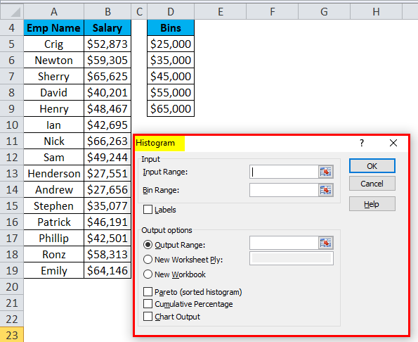
Let’s take another example with 15 data points which are the salary of a company.
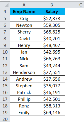
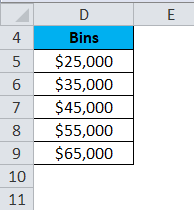
Now we will create the bins for the above dataset.
For creating the histogram chart in excel, we will follow the same steps as earlier taken in example 1.
- Click on the Data tab. Select the Data Analysis option from the Analysis section.
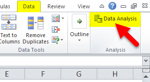
- A Data Analysis dialog box will appear. Choose the histogram option and click on OK.
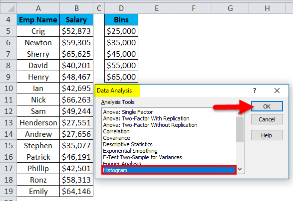
- It will open a histogram dialog box.
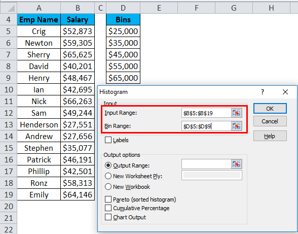
- Select the Input Range with the Salary data points.
- Select the Bin Range with the bins column.
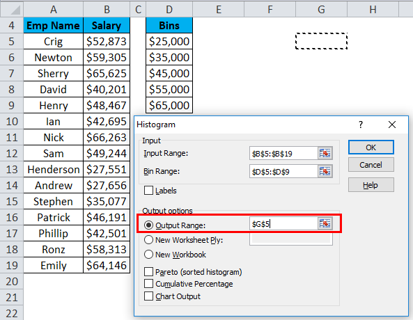
- Click on Output Range as we want to insert the chart on the same sheet and select the cell address to insert the chart.
- Choose the Chart Output option and click on OK.
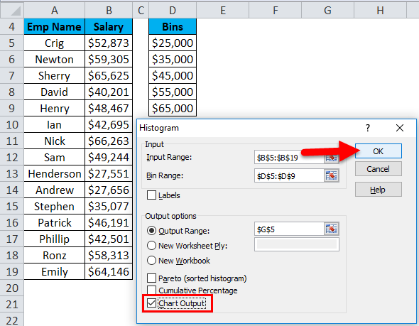
- The below chart will appear as :
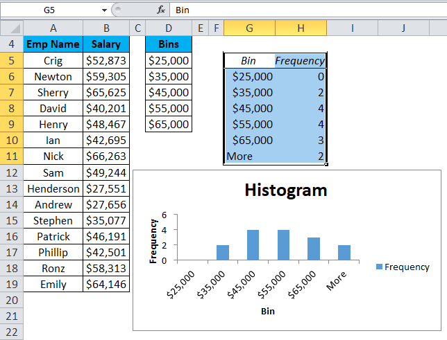
Explanation:
- The First bin, $25,000, will include all data points which are less than this value.
- The last bin More will include all the data points which are higher than $65,000. Its created automatically by Excel.
Pros
- The histogram is very useful while working with a large amount of data.
- A histogram chart shows the data in a graphical form that is easy to compare and easy to understand.
Cons
- Histogram chart is very difficult to extract the data from the input field in the histogram. It means difficult to point the exact number.
- While working with histogram, it creates a problem with multiple categories.
Things to Remember About Histogram Chart in Excel
- A Histogram chart is used for continuous data where the bin determines the range of data.
- The bins are usually determined as consecutive and non-overlapping intervals.
- The bins must be adjacent and are of equal size (but are not required to be).
- If you are working with Excel 2013, 2010 or earlier version, you need to activate the Excel Add-Ins for Data Analysis ToolPak.
Recommended Articles
This has been a guide to Histogram in Excel. Here we discuss its types and how to create a Histogram chart in Excel along with excel examples and a downloadable excel template. You may also look at these useful charts in excel –
- Marimekko Chart Excel
- Interactive Chart in Excel
- Surface Charts in Excel
- Comparison Chart in Excel
 A histogram is simply a bar graph that shows the occurrence of data intervals into a bin range. Or say it shows the frequency distributions in data.
A histogram may look like a column graph but it is not interpreted from the column’s height. It is intrepreted from the area it covers.
A bin is defined for frequency distribution. It is a kind of grouping.
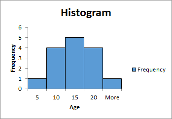
For example, if you want to know, in a school, how many students are of age 5 or below, how many are between 6-10, how many are between 11-15, how many are between 15-20 and how many are 20 or more. The histogram in excel is
the best way to analyze and visualize this data and get the answer.
Enough of the theory, let’s dig into a scenario.
How to Make a Histogram on Excel 2016 Example:
Let’s say that we have this data in excel.
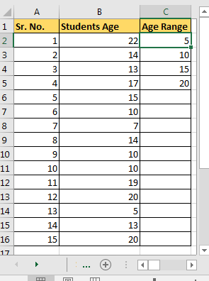
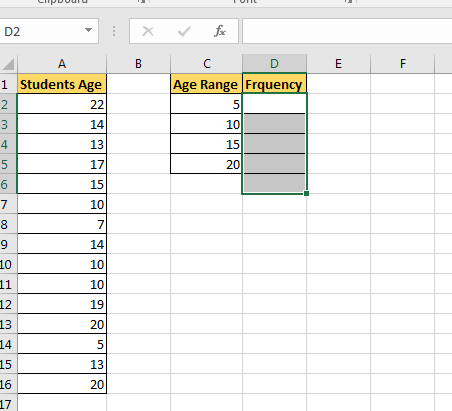
- In Column A we have Sr. No.
- In Column B we have Age.
- In Column C we have the age range or say it’s our excel histogram bin range. It shows that we want to know the number of students whose age is:
age<=5, 5<age<=10, 10<age<=15, 15<age<=20 and age>20. Simple, isn’t it? It is used to produce a frequency distribution.
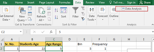
Now, to plot a histogram chart in Excel 2016, we will use Data Analysis add-in. I assume you have read how to add data Analysis Add-In Excel for adding Data Analysis Toolpak. If you have already added it in, we can continue to our histogram tutorial.
Make Histogram Using Data Analysis ToolPak
To create a histogram in Excel 2016/2013/2010 for Mac and Windows, follow these simple steps:
-
- Go to the Data tab and click on Data Analysis.
-
-
- Select Histogram in Data Analysis ToolPak Menu Dialog and hit the OK button.
-
-
-
-
- In Input Range, select your data. In Bin Range select the interval range. Now if you have selected headers then check Labels, else leave it.
-
-
Select the output range. The place where you want to show your histogram in Excel worksheets. For this example, I have selected E13 on the same sheet.
Check Chart Output checkbox for Histogram chart.
Press that OK button on top. It will plot a histogram on the excel sheet.
-
-
-
-
- Now we have created a histogram chart in Excel.
-
-
-

We need to do a little bit of editing in this chart.
-
-
-
- Select the bar and right-click. Select the format chart area. In Excel 2016 you will see this kind of menu. It is different in older versions.
-
-
Click on the little bars shown. Reduce the gap width to 0%.
-
-
-
-
- It’s done. You can also add borders to the graph to look a little bit organized. You can learn how to format the chart beautifully in excel in 2016.
-
-
-
So yeah guys. It is done. We can tell that most of the students are b/w age of 10-15 and 15-20 by just looking at this Excel Histogram chart.
How to Create Histogram in Using Formula — Dynamic Histogram
Now the biggest problem with the above method of creating Histogram in Excel, that its static. It’s good when you want to create a quick report but will be useless if your data changes from time to time. You can make this dynamic by using formula. Since it shows frequency distribution, we can use the FREQUENCY function of excel, for making excel histogram charts. Let’s see how…
So again we have that same data of students and same bin range. Now follow these steps to create a dynamic Histogram in excel 2010, 2013, and 2016 and above.
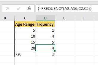
- Write heading as Frequency in the adjacent column of the bin range and select all cell adjacent to bin range. Select one extra cell to then bin range as shown in the image below. This very important.
- Now click on the formula bar and write this Frequency formula. As data array, select A2:A16 and as bin range, select C2:C5. Press Control+Shift+Enter. Yup, we need an array formula here. Make sure that you have selected a cell extra then bin range. This is for values found in more than the largest bin value. You can name it More or >20.
{=FREQUENCY(A2:A16,C2:C5)}
- Now select this bin range and frequency and goto insert tab.
- Goto chart section and select column chart. You can use a bar chart or line chart, but that’s not the traditional histogram.
- You have your dynamic histogram chart created in excel. Now, whenever you’ll change the data in excel it will change accordingly. It’s best to use named ranges for the dynamic histogram in excel.
This chart is version independent. You can create this Histogram chart in Excel 2010/2013/2016/2019/365 and any upcoming since it is based on formula instead of any version-specific feature.
How to Create Histogram Directly From Charts In Excel 2016
In Excel 2013 and 2016, we can directly create a histogram chart by using predefined histogram template in excel. It is useful when you don’t have defined bins for a histogram.
Steps to create histogram directly from the charts.
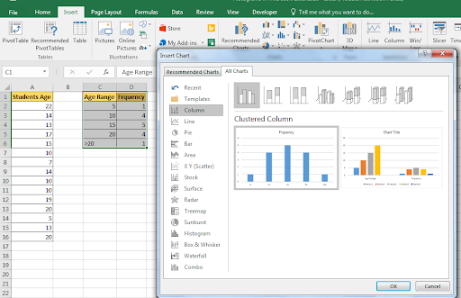
- Select data.
- Go to Insert Tab. Locate the chart section.
- Click on Recommended Charts.
- Click on All Charts.
- On the left Histogram. 4th from Bottom. There are two options. Histogram and Pareto. Select Histogram and click ok.
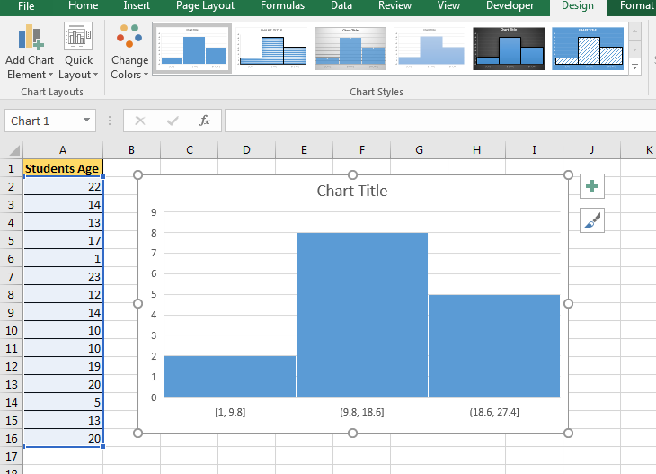
Now you have your, Histogram chart. It has predefined bins. You can customise to some extent. You can see it created 3 bins [1-9.8], (9.8-18.6], and (18.6, 27.4]. If you don want this then you can edit it.
To edit this histogram
- Right-click on bins and click Format Axis.
- You can now define your bin numbers or bin width
- There are several other options available to customize the Histogram in Excel.
I personally don’t prefer this chart. But its useful when i don’t have a bin range.
So we learned how to plot histogram in excel 2016. The histogram in Excel 2013 has the same procedure. Same case for older versions of Excel. Only the formatting options have changed.
Related Articles:
How to use the Waterfall Chart in Excel
4 Creative Target Vs Achievement Charts in Excel
How to use the Pareto Chart and Analysis In Microsoft Excel
How to do Regressions in Excel
Popular Articles:
50 Excel Shortcuts to Increase Your Productivity
How to use the VLOOKUP Function in Excel
How to use the COUNTIF function in Excel
How to use the SUMIF Function in Excel