Highlighting rows in excel - Word и Excel - помощь в работе с программами

Excel for Microsoft 365 Excel 2021 Excel 2019 Excel 2016 Excel 2013 Excel 2010 Excel 2007 More…Less

Unlike other Microsoft Office programs, such as Word, Excel does not provide a button that you can use to highlight all or individual portions of data in a cell.

However, you can mimic highlights on a cell in a worksheet by filling the cells with a highlighting color. For a fast way to mimic a highlight, you can create a custom cell style that you can apply to fill cells with a highlighting color. Then, after you apply that cell style to highlight cells, you can quickly copy the highlighting to other cells by using Format Painter.

If you want to make specific data in a cell stand out, you can display that data in a different font color or format.

Create a cell style to highlight cells

Click Home > New Cell Styles.
Notes:
- If you don’t see Cell Style, click the More button next to the cell style gallery.
In the Style name box, type an appropriate name for the new cell style.

Tip: For example, type Highlight.
Click Format.
In the Format Cells dialog box, on the Fill tab, select the color that you want to use for the highlight, and then click OK.
Click OK to close the Style dialog box.

The new style will be added under Custom in the cell styles box.
On the worksheet, select the cells or ranges of cells that you want to highlight. How to select cells?
On the Home tab, in the Styles group, click the new custom cell style you created.

Note: Custom cell styles are displayed at the top of the list of cell styles. If you see the cell styles box in the Styles group, and the new cell style is one of the first six cell styles on the list, you can click that cell style directly in the Styles group.

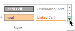
Use Format Painter to apply a highlight to other cells

Select a cell that is formatted with the highlight that you want to use.
On the Home tab, in the Clipboard group, double-click Format Painter , and then drag the mouse pointer across as many cells or ranges of cells that you want to highlight.
When you’re done, click Format Painter again or press ESC to turn it off.

Display specific data in a different font color or format

In a cell, select the data that you want to display in a different color or format.

How to select data in a cell

To select the contents of a cell	Do this
In the cell	Double-click the cell, and then drag across the contents of the cell that you want to select.
In the formula bar	Click the cell, and then drag across the contents of the cell that you want to select in the formula bar.
By using the keyboard	Press F2 to edit the cell, use the arrow keys to position the insertion point, and then press SHIFT+ARROW key to select the contents.

On the Home tab, in the Font group, do one of the following:
- To change the text color, click the arrow next to Font Color and then, under Theme Colors or Standard Colors, click the color that you want to use.
- To apply the most recently selected text color, click Font Color .
- To apply a color other than the available theme colors and standard colors, click More Colors, and then define the color that you want to use on the Standard tab or Custom tab of the Colors dialog box.
- To change the format, click Bold , Italic , or Underline .
  
  Keyboard shortcut You can also press CTRL+B, CTRL+I, or CTRL+U.

Need more help?

Want more options?

Explore subscription benefits, browse training courses, learn how to secure your device, and more.

Communities help you ask and answer questions, give feedback, and hear from experts with rich knowledge.

Источник

1
Open the spreadsheet you want to edit in Excel. You can usually do this by double-clicking the file on your PC.
- This method is suitable for all types of data. You’ll be able to edit your data as needed without affecting the formatting.
2
Select the cells you want to format. Click and drag the mouse so that all cells in the range you want to style are highlighted.^[1]
- To highlight every other row of the entire document, click the Select All button, which is the gray square button/cell at the top-left corner of the sheet.
Advertisement
3

Click the

icon next to «Conditional Formatting.« It’s on the Home tab in the toolbar that runs along the top of the screen. A menu will expand.
4

Click New Rule. This opens the “New Formatting Rule” dialog box.
5
Select Use a formula to determine which cells to format. You’ll find this option under “Select a Rule Type.”
- If you’re using Excel 2003, set “condition 1” to «Formula is.»
6
Enter the formula to highlight alternating rows. Type the following formula into the typing area:^[2]
- =MOD(ROW(),2)=0
7

Click Format. It’s a button on the dialog box.
8

Click the Fill tab. It’s at the top of the dialog box.
9

Select a pattern or color for the shaded rows and click OK. You’ll see a preview of the color below the formula.
10
Click OK. This highlights alternating rows in the spreadsheet with the color or pattern you selected.
- You can edit your formula or formatting by clicking the arrow next to Conditional Formatting (on the Home tab), selecting Manage Rules, and then selecting the rule.

1

Open the spreadsheet you want to edit in Excel. You can usually do this by double-clicking the file on your Mac.
2
Select the cells you want to format. Click and drag the mouse to select all the cells in the range you want to edit.
- If you want to highlight every other row in the entire document, press ⌘ Command+A on your keyboard. This will select all the cells in your spreadsheet.
3

Click the

icon next to «Conditional Formatting.« You can find this button on the Home toolbar at the top of your spreadsheet. It will expand your formatting options.
4

Click New Rule on the Conditional Formatting menu. This will open your formatting options in a new dialogue box, titled «New Formatting Rule.»
5

Select Classic next to Style. Click the Style drop-down in the pop-up window, and select Classic at the bottom of the menu.
6

Select Use a formula to determine which cells to format under Style. Click the drop-down below the Style option, and select the Use a formula option to customize your formatting with a formula.
7
Enter the formula to highlight alternating rows. Click the formula field in the New Formatting Rule window, and type the following formula: ^[3]
- =MOD(ROW(),2)=0
8
Click the drop-down next to Format with. This option is located below the formula field at the bottom. It will expand your formatting options on a drop-down.
- The formatting you select here will be applied to every other row in the selected area.
9
Select a formatting option on the «Format with» drop-down. You can click an option here, and preview it on the right-hand side of the pop-up window.
- If you want to manually create a new highlight format with different color, click the custom format… option at the bottom. It will open a new window, and allow you to manually select fonts, borders and colors to use.
10
Click OK. This will apply your custom formatting, and highlight every other row in the selected area on your spreadsheet.
- You can edit the rule at any time by clicking the arrow next to Conditional Formatting (on the Home tab), selecting Manage Rules, and then selecting the rule.

1
Open the spreadsheet you want to edit in Excel. You can usually do this by double-clicking the file on your PC or Mac.
- Use this method if you want to add your data to an browsable table in addition to highlighting every other row.
- You should only use this method only if you won’t need to edit the data in the table after applying the style.
2

Select the cells you want to add to the table. Click and drag the mouse so that all cells in the range you want to style are highlighted.^[4]
3

Click Format as Table. It’s on the Home tab on the toolbar that runs along the top of the app.^[5]
4

Select a table style. Scroll through the options in the Light, Medium, and Dark groups, then click the one you want to use.
5
Click OK. This applies the style to the selected data.
- You can edit the style of the table by selecting or deselecting preferences in the “Table Style Options” panel on the toolbar. If you don’t see this panel, click any cell in the table and it should appear.
- If you want to convert the table back to a regular range of cells so you can edit the data, click the table to bring up the table tools in the toolbar, click the Design tab, then click Convert to Range.

Ask a Question

200 characters left

Include your email address to get a message when this question is answered.

Submit

Thanks for submitting a tip for review!

wikiHow Video: How to Highlight Every Other Row in Excel

About This Article

Article SummaryX

1. Highlight the data you want to format.
2. Click the arrow next to «Conditional Formatting.»
3. Click New Rule.
4. Select Use a formula to determine which cells to format.
5. Enter this formula: =MOD(ROW(),2)=0
6. Click Format.
7. Select a color on the Fill tab.
8. Click OK and then OK again.

Did this summary help you?

Thanks to all authors for creating a page that has been read 228,525 times.

Is this article up to date?

Источник

Conditional Formatting generally checks the value in one cell and applies formatting over the other cells. A great application of conditional formatting is highlighting the entire row or multiple rows based on a cell value and condition provided in the formula.

It is very helpful because for a data set with tons of value in it becomes cumbersome to analyze just by reading the data. So, if we highlight a few rows based on some conditions, it becomes easier for the user to infer from the data set. For example, in a college, some students have been blacklisted due to some illegal activities. So, in the Excel record the administrator can highlight the rows where these students records are present.

In this article we are going to see how to highlight row(s) based on cell value(s) using a suitable real time example shown below :

Example : Consider a company’s employees data is present. The following table consists of data about the project(s) which has been assigned to employees, their ages and ID. An employee can work on multiple projects. The blank cell in project denotes that no project has been assigned to that employee.

Highlighting the Rows

1. On the basis of text match :

Aim : Highlight all the rows where Employee name is “Srishti”.

Steps :

1. Select the entire dataset from A3 to D14 in our case.

2. In the Home Tab select Conditional Formatting. A drop-down menu opens.

3. Select New Rule from the drop-down. The dialog box opens.

4. In the New Formatting Rule dialog box select “Use a Formula to determine which cells to format” in the Select a Rule Type option.

5. In the formula box, write the formula :

=$B2="Srishti"

$ is used to lock the column B, so that only the cell B is looked starting from Row 2

The formula will initially check if the name “Srishti” is present or not in the cell B2. Now, since cell B is locked and next time checking will be done from cell B3 and so on until the condition gets matched.

6. In the Preview field, select Format and then go to Fill and then select an appropriate color for highlighting and click OK

7. Now click OK and the rows will be highlighted.

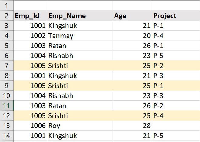
Highlighted Rows

2. Non-text matching based on number :

Aim : Highlight all the rows having age less than 25.

Approach :

Repeat the above steps as discussed and in the formula write :

=$C3<25

Highlighted Rows

3. On the basis of OR/AND condition :

OR, AND are used when we have multiple conditions. These are logical operators which work on True value.

AND : If all conditions are TRUE, AND returns TRUE.

OR : At least one of the conditions needs to be TRUE to return TRUE value.

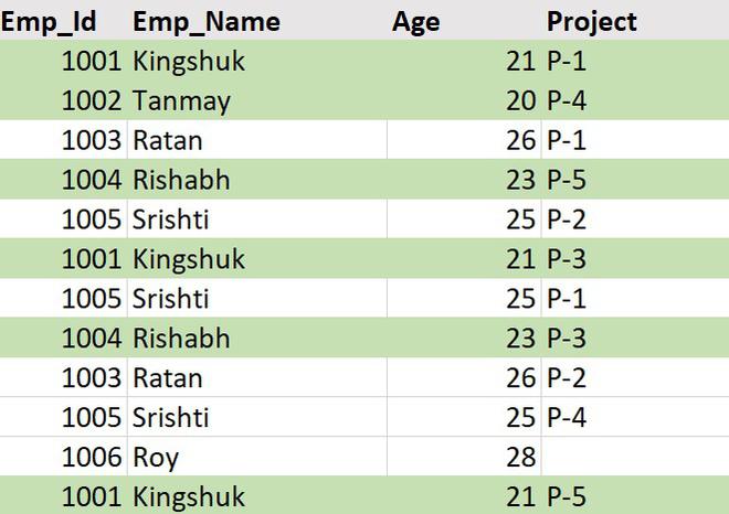
Aim : Highlight all the rows of employees who are either working on Project 1 or Project 4.

The project details are in column D. So, the formula will be :

=OR($D3="P-1",$D3="P-4")

Aim : Suppose employee Rishabh has completed the project P-3. The administrator is asked to highlight the row and keep a record of projects which are finished.

The name is in column B and the project details is in column D. The formula will be :

=AND($B3="Rishabh",$D3="P-3")

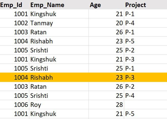
Highlighted Row

4. On the basis of any blank row :

Aim : Check if there is/are any blank row(s). If exist(s), then highlight it.

The project details is in column D. We will use the COUNTIF( ) function to check for the number of blank records. The formula will be :

=COUNTIF($A3:$D3,"")>0

"" : Denotes blank

The above formula checks all the columns one by one and sees if there is at least one blank row. If the formula value is greater than zero then highlighting will be done else COUNTIF will return FALSE value and no highlighting will be done.

5. On the basis of multiple conditions and each condition having different color :

Aim : Suppose the company wants to distinguish the employees based on their ages. The employees whose age is more than 25 are senior employees and whose age is more than 20 but less than or equal to 25 are junior developers or trainees. So, the administrator is asked to highlight these two categories with different colors.

Implementation :

In the Formula Field write the formula :

=$C3>25

This will highlight all the rows where age is more than 25.

Again in the Formula Field write the formula :

=$C3>20

This will highlight all the rows greater than 20. It will in fact change the color of the rows where age is greater than 25. Since, if a number is greater than 20 then definitely it is greater than 25. So, all the cells having age more than 20 will be highlighted to the same color.

This creates a problem as our goal is to make two separate groups. In order to resolve this we need to change the priority of highlighting the rows. The steps are :

Undo the previous steps using CTRL+Z.
Select the entire dataset.
Go to Conditional Formatting followed by Manage Rules.

In the Manage Rule dialog box :

The order of the condition needs to be changed. The condition at the top will have more priority than the lower one. So, we need to move the second condition to the top of the first one using the up icon after selecting the condition.

Now click on Apply and then OK.

It can be observed that the rows are now divided into two categories : The yellow color is for the senior level employees and the green color is for junior employees and trainees in the company on the basis of their ages.

Источник

Hi i know that «SHIFT + spacebar» ‘highlights’ an excel row. But what I want to do is actually to ‘highlight’ it such that the background is yellow. Is there a keyboard shortcut for that?

SeanC

3,6292 gold badges19 silver badges26 bronze badges

asked Sep 19, 2012 at 7:33

You can just click on the row number so that the entire row is selected.Now just go to the fill color option, choose your desired color, and the entire row will be highlighted.

jonsca

4,07715 gold badges34 silver badges46 bronze badges

answered Sep 19, 2012 at 7:53

i’m looking for a shortcut also. the only method I found so far is the F4 button. it mimics your last action.

So I would suggest:
highlight with color the row you want, and select another row you want to highlight with the same color and press F4.

answered May 9, 2017 at 17:35

You click the little paint bucket icon in the ribbon, in the Font section. There is a little arrow next to it which gives you an option to change the colour.

answered Sep 19, 2012 at 7:39

paradroidparadroid

22.5k10 gold badges72 silver badges113 bronze badges

If you press Alt on any Office program, small key-symbols appear on the ribbon tabs. If you press one of those keys, more symbols appear on that tab’s buttons. Those symbols denote the shortcuts for the buttons. So, each shortcut consists of three key presses after each other:

Alt
The tab’s shortcut key.
The button’s shortcut key.

answered Sep 20, 2012 at 6:57

The shortcut to select highlight in excel 2013 for windows is Alt H + H (hold down ALT and tap H twice). Probably works on other versions with the ribbon.

This works well for highlighting rows too, just use the shortcut to select a row in Excel — Shift + Space Bar, followed by the highlight shortcut (Alt + H + H)

answered Oct 25, 2017 at 9:37

Источник