
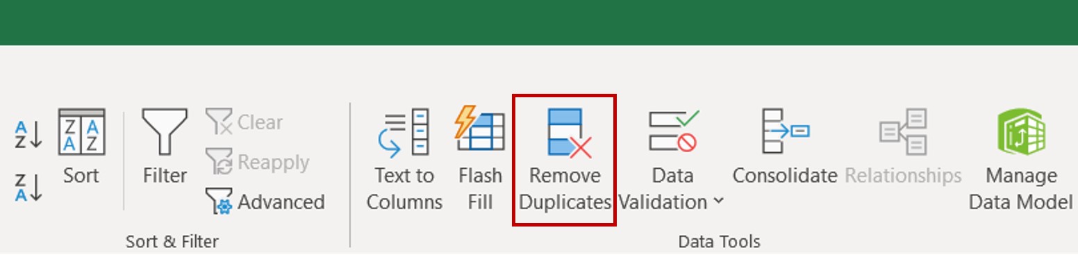
Find and remove duplicates
Excel for Microsoft 365 Excel 2021 Excel 2019 Excel 2016 Excel 2013 Excel 2010 Excel 2007 Excel Starter 2010 More…Less
Sometimes duplicate data is useful, sometimes it just makes it harder to understand your data. Use conditional formatting to find and highlight duplicate data. That way you can review the duplicates and decide if you want to remove them.
-
Select the cells you want to check for duplicates.
Note: Excel can’t highlight duplicates in the Values area of a PivotTable report.
-
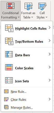
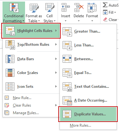
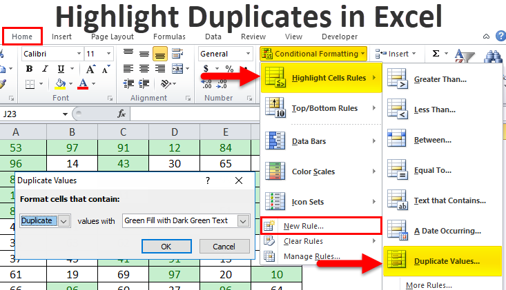
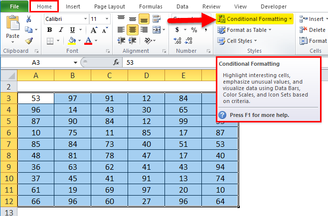
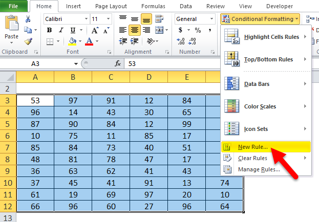
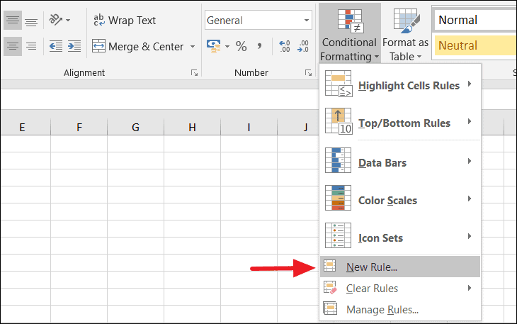
Click Home > Conditional Formatting > Highlight Cells Rules > Duplicate Values.

-
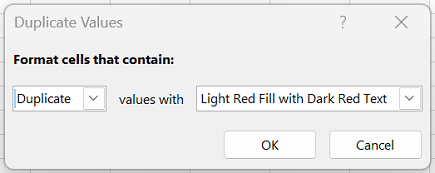
In the box next to values with, pick the formatting you want to apply to the duplicate values, and then click OK.
Remove duplicate values
When you use the Remove Duplicates feature, the duplicate data will be permanently deleted. Before you delete the duplicates, it’s a good idea to copy the original data to another worksheet so you don’t accidentally lose any information.
-
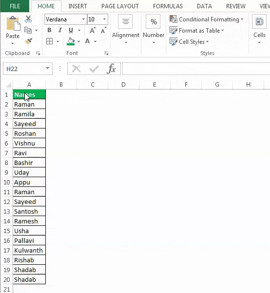
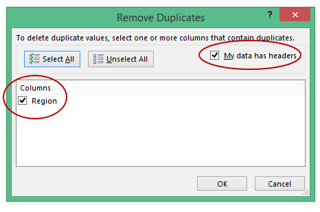
Select the range of cells that has duplicate values you want to remove.
-
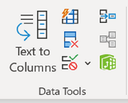
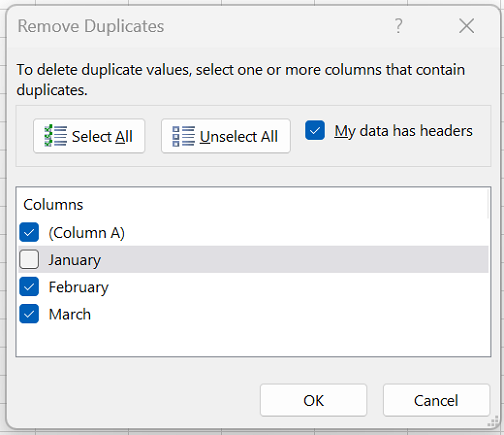
Click Data > Remove Duplicates, and then Under Columns, check or uncheck the columns where you want to remove the duplicates.
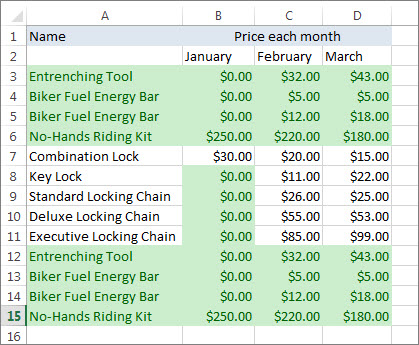
For example, in this worksheet, the January column has price information I want to keep.
So, I unchecked January in the Remove Duplicates box.
-
Click OK.
Note: The counts of duplicate and unique values given after removal may include empty cells, spaces, etc.
Need more help?

Need more help?
Want more options?
Explore subscription benefits, browse training courses, learn how to secure your device, and more.
Communities help you ask and answer questions, give feedback, and hear from experts with rich knowledge.
What is Highlight Duplicate Values in Excel?
A duplicate value occurs more than once in a dataset. It is often found while working with large databases in excel. It is essential to find and highlight the duplicate values in excel because the user may or may not want to retain them.
For example, Jennifer creates a list of expenditures incurred on fruits and vegetables for a particular month. Since the leftover amount varies from the actual in-hand balance, she examines the list again.
Jennifer notices that $18 spent on apples has been mistakenly entered twice. Hence, it is essential to identify duplicates in a series of data values. This helps deal with the duplicates accordingly.
The purpose of highlighting duplicates in excel is to make the data understandable and accurate. Moreover, it helps in differentiating the unique values from the duplicated ones.
Prior to deleting the duplicates permanently, it is recommended to keep a copy of the original data. This allows one to return to the source data, if required.
Table of contents
- What is Highlight Duplicate Values in Excel?
- How to Highlight Duplicate Values in Excel?
- Example #1–Highlight Current Duplicates in the Selected Excel Range
- Example #2–Highlight Future Duplicates in the Selected Range
- Example #3–Remove Duplicates From the Selected Range
- The Cautions Governing Duplicate Values
- Frequently Asked Questions
- Recommended Articles
- How to Highlight Duplicate Values in Excel?
How to Highlight Duplicate Values in Excel?
We can highlight the duplicate values in a single excel column as well as in an entire worksheet. The difference between the former and the latter is in the selection of cells. Hence, one must be careful while selecting cells in the first step.
Let us consider a few examples.
Example #1–Highlight Current Duplicates in the Selected Excel Range
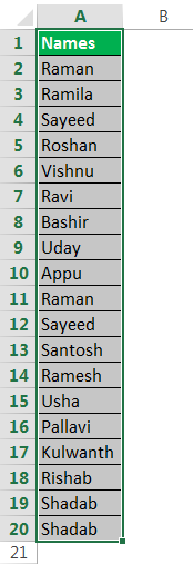
The following table shows the list of names of a few people. We want to find and highlight the current duplicates with the help of conditional formattingConditional formatting is a technique in Excel that allows us to format cells in a worksheet based on certain conditions. It can be found in the styles section of the Home tab.read more.
The steps to find and highlight the duplicates in excel by using conditional formatting are listed as follows:
- Select the data range that consists of the duplicate values.
Note: In this case, ensure that only the particular range containing duplicates is selected and not the entire worksheet.

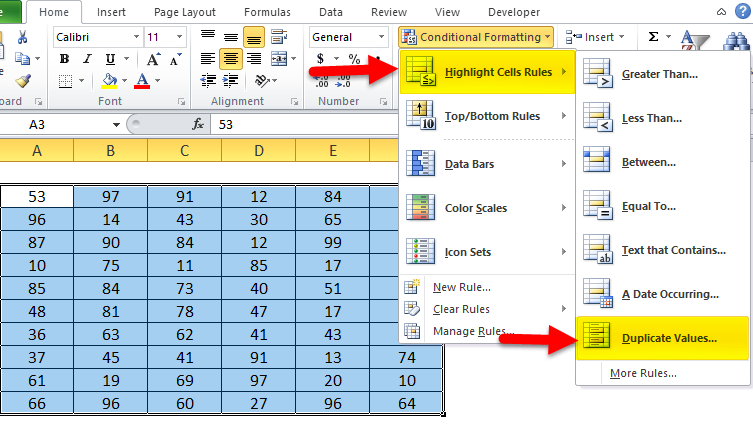
- Click the conditional formattingConditional formatting is a technique in Excel that allows us to format cells in a worksheet based on certain conditions. It can be found in the styles section of the Home tab.read more drop-down under the “styles” group of the Home tab. In “highlight cells rules,” select duplicate values, as shown in the following image.
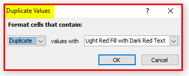
- The “duplicate values” dialog box opens, as shown in the following image. One can choose the required type of formattingFormatting is a useful feature in Excel that allows you to change the appearance of the data in a worksheet. Formatting can be done in a variety of ways. For example, we can use the styles and format tab on the home tab to change the font of a cell or a table.read more in the “values with” box.
It is possible to highlight either the cell, the text or both with different colors. One can also highlight the borders of the cells containing duplicates.

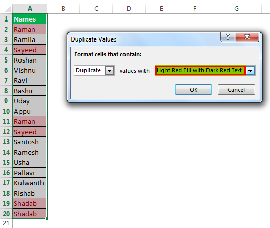
- Select “light red fill with dark red text” and click “Ok.” The values occurring more than once in the selected range (column A) are highlighted, as shown in the following image.
Note: The conditional formatting feature highlights the duplicate values including their first occurrence.


Example #2–Highlight Future Duplicates in the Selected Range
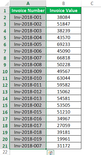
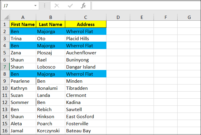
The succeeding table consists of the invoice numbers and the corresponding amounts. On a selected range, we want to perform both the following tasks:
- Highlight the current duplicate values
- Highlight the duplicate values to be entered in the future
Use the conditional formatting feature of Excel.
The steps to highlight the current and the future duplicate values by using conditional formatting are listed as follows:
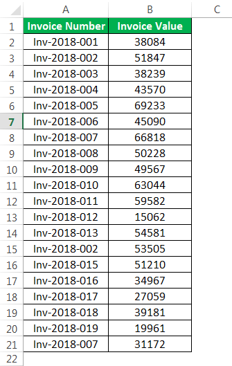
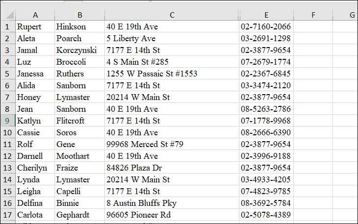
Step 1: Select the column “invoice number” (column A). With this selection, it will be possible to highlight the new duplicate value entered in the existing list (column A) in future.
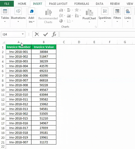
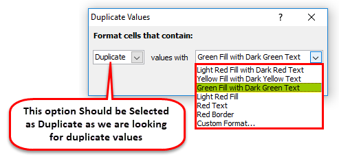
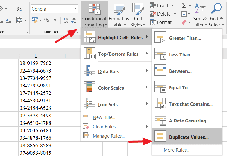
Step 2: In the Home tab, click the conditional formatting drop-down under the “styles” group. Select “duplicate values” from “highlight cells rules,” as shown in the following image.
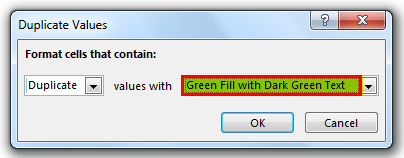
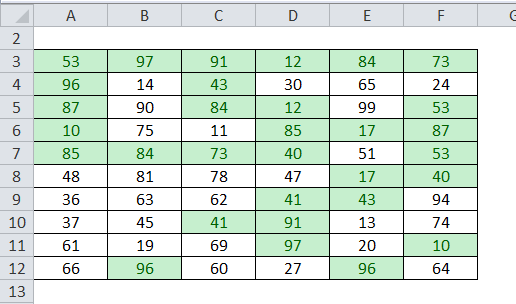
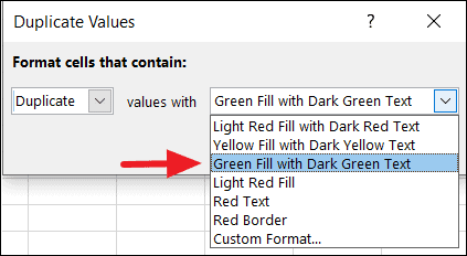
Step 3: Select the color in which the duplicate cell values are to be highlighted. We select “green fill with dark green text.” Click “Ok.”
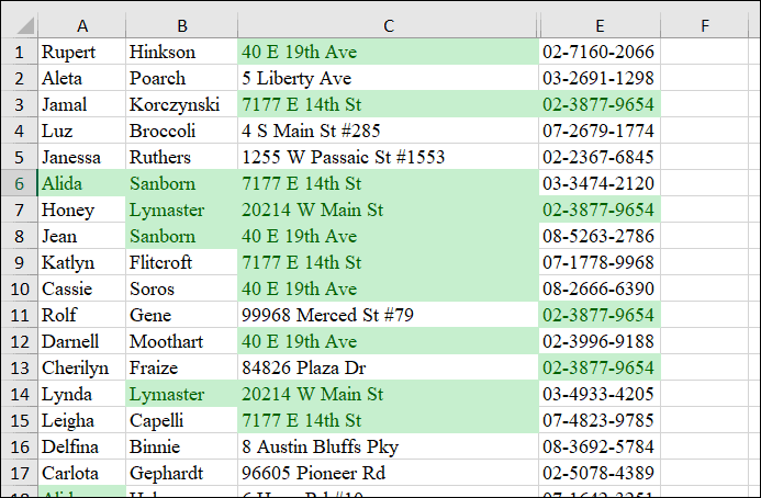
Step 4: Four duplicate values are highlighted in green. These are the ones that are occurring more than once.
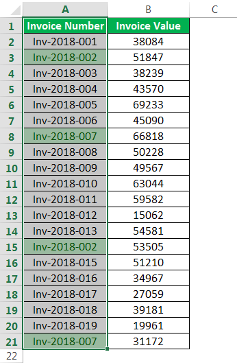
Step 5: Enter any of the duplicate invoice numbers in row 22 of column A. The new duplicate entry of column A is highlighted automatically, as shown in the succeeding image.
Note 1: Alternatively, select the entire worksheet (in step 1) and perform the steps 2 and 3. The results will be the same as those obtained in step 4.
Note 2: There is a difference between selecting a specific column and the worksheet. In the former, the duplicate value entered in a new cell of the same column will be highlighted. In contrast, if a worksheet is selected, the duplicate value entered in any cell of this worksheet will be highlighted.

Example #3–Remove Duplicates From the Selected Range
Working on the data of example #1, we want to remove the duplicates from the selected range.
The steps to remove duplicates from a selected range are listed as follows:
Step 1: Select the data range containing duplicates.
Step 2: Click “remove duplicates” from the “data tools” group of the Data tab.
Alternatively, press the shortcut keys “Alt+A+M” one by one.

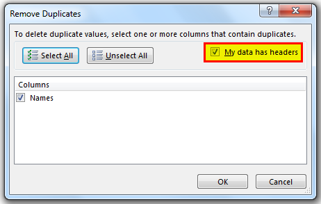
Step 3: The “remove duplicatesTo remove duplicates from the excel column, the user can adopt any of the three well-known methods: Using data tools group, Using the advanced filter in excel, Conditional formatting in excel.read more” dialog box appears, as shown in the following image. The box under “columns” shows the header of the selected column.
Select the checkbox “my data has headers.” Click “Ok.”
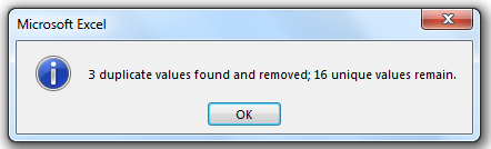
Step 4: The duplicate values are removed from the selected column (column A). A message appears stating the number of duplicates deleted and the number of unique values retained.
Click “Ok” to see the results.
Step 5: The column A now shows only the unique data values. Hence, the duplicate values have been removed.

The Cautions Governing Duplicate Values
The cautions to be observed while dealing with duplicates are listed as follows:
- Make sure to select the correct range in which duplicates are to be highlighted.
- Ensure that you select the “custom format” option in the “duplicate values” dialog box to choose the formatting style of the duplicate cells.
- Remember to select the correct column header while removing the duplicates.
Frequently Asked Questions
1. What does it mean to highlight duplicates and how is it done in Excel?
A duplicate value occurs more than once in a dataset. Duplicates are highlighted in order to make the data understandable. Moreover, highlighting allows the user to review every duplicate value and decide whether to retain or remove it.
The steps to find and highlight duplicates in excel are listed as follows:
a. Select the range in which duplicates are to be found and highlighted.
b. Click the “conditional formatting” drop-down from the Home tab of Excel. Select “duplicate values” from “highlight cells rules.”
c. The duplicate values” box opens. Select the required formatting from the various options available in the “values with” box. Click “Ok.”
The duplicates within the selected range are found and highlighted with the color selected in step c.
2. How to highlight duplicates in multiple columns of Excel?
Let us highlight duplicates in the following columns:
• Column A consists of rose, lily, sunflower, lily, and lotus in the range A1:A5.
• Column B consists of tulip, rose, orchid, lotus, and rose in the range B1:B5.
• Column C consists of sunflower, daffodil, marigold, tulip, and hibiscus in the range C1:C5.
The steps to highlight duplicates in the excel columns A, B, and C are listed as follows:
a. Select the range A1:C5.
b. Click the “conditional formatting” drop-down from the Home tab. Select “manage rules.”
c. The “conditional formatting rules manager” dialog box opens. Click “new rule.”
d. Under “select a rule type,” click “format only unique or duplicate values.” Under “format all,” select “duplicate.”
e. Click “format” and select the required color in the “fill” tab. Click “Ok.”
f. Click “Ok” again in the “new formatting rule” window.
g. The rule applied to the current selection appears in the “conditional formatting rules manager” dialog box. Click “Ok.”
All the flower names occurring more than once in the selected range (A1:C5) are highlighted. The unique flower names are orchid, daffodil, marigold, and hibiscus. The remaining flower names are duplicate values.
Note: The mentioned procedure highlights the duplicate values including their first occurrence.
3. How to highlight duplicates in multiple columns with an Excel formula?
The steps for highlighting duplicates in multiple columns with the COUNTIF formula are listed as follows:
a. Select the entire range in which duplicates are to be found.
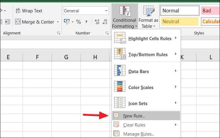
b. Click the “conditional formatting” drop-down from the Home tab. Select “new rule.”
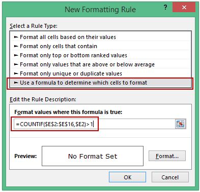
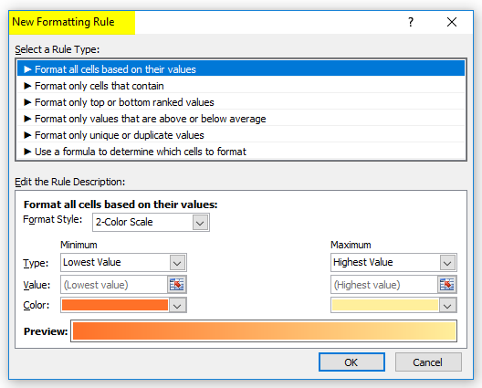
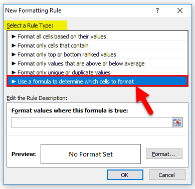
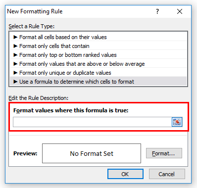
c. The “new formatting rule” window opens. Choose the option “use a formula to determine which cells to format” under “select a rule type.”
d. Under “edit the rule description,” enter the following formula.
“=COUNTIF(range,top_cell)>1”
The “range” is the selected range of step a. The “top_cell” is the first, leftmost cell of the current selection. For instance, if the “range” is A1:C5, the formula becomes “=COUNTIF($A$1:$C$5,A1)>1.”
e. Click “format” and select the desired color (in the “fill” tab) for highlighting duplicates. Click “Ok.”
f. Click “Ok” again in the “new formatting rule” window.
The duplicates in the selected range are highlighted.
Note: In the formula entered in step d, the “range” ($A$1:$C$5) is written using absolute references. The “top_cell” (A1) is written using relative reference.
Recommended Articles
This has been a guide to guide to Highlight Duplicates in Excel. Here we discuss how to find and highlight duplicate values in excel with step by step examples You may learn more about Excel from the following articles-
- Excel Borders
- Highlight Every Other Excel Row
- Removing Duplicates in Excel
- Advanced Filter in Excel
Duplicate Values | Triplicates | Duplicate Rows
This example teaches you how to find duplicate values (or triplicates) and how to find duplicate rows in Excel.
Duplicate Values
To find and highlight duplicate values in Excel, execute the following steps.
1. Select the range A1:C10.

2. On the Home tab, in the Styles group, click Conditional Formatting.

3. Click Highlight Cells Rules, Duplicate Values.

4. Select a formatting style and click OK.

Result. Excel highlights the duplicate names.

Note: select Unique from the first drop-down list to highlight the unique names.
Triplicates
By default, Excel highlights duplicates (Juliet, Delta), triplicates (Sierra), etc. (see previous image). Execute the following steps to highlight triplicates only.
1. First, clear the previous conditional formatting rule.
2. Select the range A1:C10.
3. On the Home tab, in the Styles group, click Conditional Formatting.
4. Click New Rule.

5. Select ‘Use a formula to determine which cells to format’.
6. Enter the formula =COUNTIF($A$1:$C$10,A1)=3
7. Select a formatting style and click OK.

Result. Excel highlights the triplicate names.

Explanation: =COUNTIF($A$1:$C$10,A1) counts the number of names in the range A1:C10 that are equal to the name in cell A1. If COUNTIF($A$1:$C$10,A1) = 3, Excel formats cell A1. Always write the formula for the upper-left cell in the selected range (A1:C10). Excel automatically copies the formula to the other cells. Thus, cell A2 contains the formula =COUNTIF($A$1:$C$10,A2)=3, cell A3 =COUNTIF($A$1:$C$10,A3)=3, etc. Notice how we created an absolute reference ($A$1:$C$10) to fix this reference.
Note: you can use any formula you like. For example, use this formula =COUNTIF($A$1:$C$10,A1)>3 to highlight names that occur more than 3 times.
Duplicate Rows
To find and highlight duplicate rows in Excel, use COUNTIFS (with the letter S at the end) instead of COUNTIF.
1. Select the range A1:C10.

2. On the Home tab, in the Styles group, click Conditional Formatting.
3. Click New Rule.
4. Select ‘Use a formula to determine which cells to format’.
5. Enter the formula =COUNTIFS(Animals,$A1,Continents,$B1,Countries,$C1)>1
6. Select a formatting style and click OK.

Note: the named range Animals refers to the range A1:A10, the named range Continents refers to the range B1:B10 and the named range Countries refers to the range C1:C10. =COUNTIFS(Animals,$A1,Continents,$B1,Countries,$C1) counts the number of rows based on multiple criteria (Leopard, Africa, Zambia).
Result. Excel highlights the duplicate rows.

Explanation: if COUNTIFS(Animals,$A1,Continents,$B1,Countries,$C1) > 1, in other words, if there are multiple (Leopard, Africa, Zambia) rows, Excel formats cell A1. Always write the formula for the upper-left cell in the selected range (A1:C10). Excel automatically copies the formula to the other cells. We fixed the reference to each column by placing a $ symbol in front of the column letter ($A1, $B1 and $C1). As a result, cell A1, B1 and C1 contain the same formula, cell A2, B2 and C2 contain the formula =COUNTIFS(Animals,$A2,Continents,$B2,Countries,$C2)>1, etc.
7. Finally, you can use the Remove Duplicates tool in Excel to quickly remove duplicate rows. On the Data tab, in the Data Tools group, click Remove Duplicates.

In the example below, Excel removes all identical rows (blue) except for the first identical row found (yellow).


Note: visit our page about removing duplicates to learn more about this great Excel tool.

A duplicate value is a value that shows up more than once in a spreadsheet. These pop up all the time when working with datasets, and they can be tedious to sort through if you don’t know the quick ways to find them. Learn how to highlight duplicates in Excel to make the process take less than a minute!
You can even customize your settings to include only the second or third time the data appears, or highlight only specific types of duplicates. There are several ways to get the job done – we’ll use the same table in each example to keep things simple.
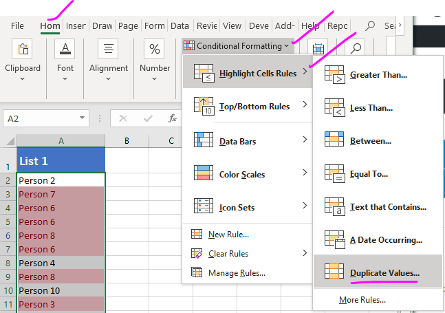
1. Highlight duplicates in a range of cells
One easy way to highlight duplicates in Excel is to use conditional formatting. Here’s how to do it:
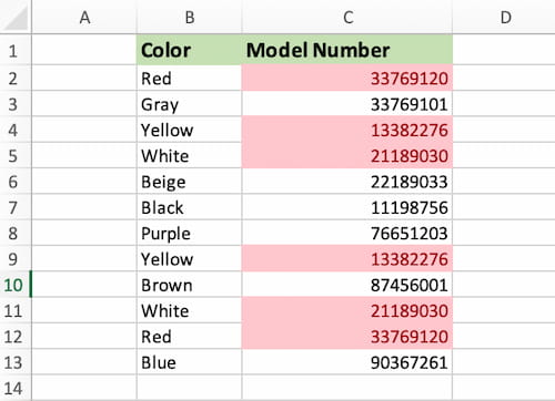
- Enter your values and select the range where you want to find the duplicates. In this example, the range is C2:C13.
Note: You can download this sample file to save some time instead of typing in all the values manually:
- Navigate over to the Home Ribbon item and select Conditional Formatting.
- Select Highlight Cells Rules and choose to highlight duplicate values. You can use several colors to highlight the cell, the text, or both.
- The final result will look like this:
If you want to continue highlighting duplicates in your Excel spreadsheet as the list grows, just select column C and follow the same steps!
2. Highlight All Duplicate Values Except One
Let’s say you need to delete all duplicates from a spreadsheet but want to keep all unique values. If it has a lot of duplicates, it would still require you to manually sift through all the highlights to figure out which ones to get rid of.
By highlighting all duplicate values in Excel except for one, you’ll be able to easily see which ones can be kept and which ones can be eliminated.
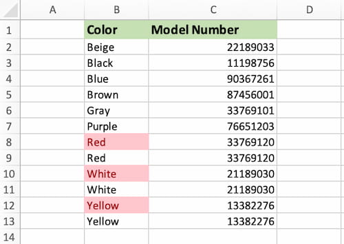
- Start by using Sort & Filter to order column B alphabetically. This just makes it easier to compare the values.
- Select column B.
- Select Conditional Formatting and Highlight Cells Rules.
- From the drop-down menu, choose Use a formula to determine which cells to format.
- Insert the following formula: =COUNTIF($B$2:$B2,$B2)>1
- Choose your highlight color and click OK.
And that’s it!
The COUNTIF function is used to count the number of cells that meet a certain criteria. In this case, the criteria is that the number of times a value is referenced is greater than 1 (seen as >1 in the above formula).
You can use nearly the same formula to highlight data that only appears a second time:
=COUNTIF($B$2:$B2,$B2)=2
=COUNTIF($B$2:$B2,$B2)=3 can be used to highlight data that appears a third time, and so on.
3. Check multiple columns for duplicates
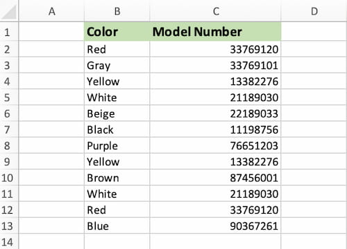
If you have a table with two columns or more and want to check for duplicates in the rows, the first two methods won’t work.
Our example table consists of two columns. So, Excel has to take both the Color and Model Number into consideration. We’ll also create a new column that merges the data.
- In cell D2, enter the formula =CONCAT(B2,C2). This column will contain the merged data.
- Use autofill to finish filling in the rest of the cells from D2:D13.
- Select all cells from B2:D13.
- Select Conditional Formatting and Highlight Cells Rules.
- From the drop-down menu, choose Use a formula to determine which cells to format. Choose a highlight color if you’d like.
- Enter the formula =COUNTIF($D$1:$D$13,$D1)>1 and select OK.
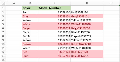
The final result will look like that!
4. Highlight Consecutive Duplicate Values Only
Maybe you have a worksheet that has a few duplicates sprinkled in, but you only want to highlight the ones that are right next to each other in your dataset. There’s an easy way to do that, too!
- As usual, first select your data. That will be B2:B13 in this case.
- Select Conditional Formatting and Highlight Cells Rules.
- From the drop-down menu, choose Use a formula to determine which cells to format.
- Enter the formula =OR(B2=B1,B2=B3)
- Select the formatting style you want and select OK.

Now, if your duplicate values aren’t consecutive, you won’t see any highlights. Head over to Sort & Filter, sort them alphabetically, and then you’ll see all the highlights pop up.
If you try adding a non-consecutive duplicate – like a new row with Red up top – you’ll see that that one isn’t highlighted as it’s not beside the others.
There are more ways to highlight Duplicates in Excel, but these methods are simple enough for everyday use and usually take less than a minute once you’ve got a little practice.
Do you have any other interesting ways to highlight duplicates in Excel? Let us know in the comments!
-
Excel
Guide to Understanding How to Highlight Duplicate Values in Excel
How to Highlight Duplicate Values in Excel
The following tutorial demonstrates the process of how to highlight duplicate values in Excel using the built-in conditional formatting feature.
This automated process can make sorting through and understanding a data set far more efficient.

How to Highlight Duplicate Values in Excel (Step-by-Step)
The quickest and most convenient method of identifying and highlighting duplicates in a data set is to utilize the conditional formatting feature in Excel.
Conditional formatting provides the ability to highlight duplicate entries, after which the user can either remove the duplicates or keep them as-is.
Duplicate values can often be the result of a system or error arising from manual entry, which in most cases would be subsequently removed.
On the other hand, the duplicate entries could be a normal occurrence (and thus might not need to be removed). For instance, a company might be wanting to identify recurring customers that have placed multiple orders in the past.
One side benefit of utilizing conditional formatting in Excel is that not only are duplicate values in the current range highlighted, but the conditional formatting can continuously check for duplicates as new entries roll-in, assuming the rule is set properly.
The process of highlighting the duplicate values in a selected range of data can be broken into four steps:
- Step 1 → Open the “Home” Tab
- Step 2 → Click on “Conditional Formatting” (Styles Group)
- Step 3 → Select “Highlight Cells Rules”
- Step 4 → Click on Duplicate Values…
Highlighting Duplicate Values with Conditional Formatting
The “Conditional Formatting” selection can be found on the Home tab in Excel, within the Styles group.

Within “Conditional Formatting”, the next step is to open the “Highlight Cell Rules” group, which displays a variety of rules that could be applied.
Near the bottom of the list, the “Duplicate Values…” selection is the one that we want to select, which should open the formatting style box in which duplicate entries will appear.
Upon clicking on “Duplicate Values…”, the following box should appear. You can either proceed with the default formatting setting (i.e. “Light Red Fill with Dark Red Text”) or customize the style.

If applicable to the task at hand, once the duplicate entries are highlighted, the “Remove Duplicates” option can then be selected in the “Data” tab (and “Data Tools” group”).
Highlight Duplicate Values Keyboard Shortcut
The following keyboard shortcut can be used to make the process above even more efficient.
Highlight Duplicate Values Shortcut = ALT → H → L → H → D
Note that each key should be pressed separately, not simultaneously.
Highlighting Duplicate Values with Excel COUNTIF Function
An alternative method to highlighting duplicate values is to create a formula-based rule.
By clicking on “New Rule”, rather than “Duplicate Values…”, the option to create a new formatting rule appears.
Selecting “Use a formula to determine which cells to format” shows the option to enter a custom formula in the “Format values where this formula is true”.
The formula used to highlight the duplicate values is as follows.
=COUNTIF(range, criteria)>1
- “range” → The selected range of cells in which the rule will find and highlight duplicates. In order for the conditional formatting to function correctly, the range must be anchored, i.e. an absolute reference (F4).
- “criteria” → The active cell can be any cell reference in the range. Unlike the range, the active cell should NOT be an absolute reference, as the formula is automatically copied across all cells in the chosen range.
If you want to highlight only the duplicates that appear more than two times, the “>1” can be replaced with “>2” – or if you want to highlight only values with an exact given number of duplicates, simply switch the “>” with “=”.
In comparison to the prior method, setting a custom rule tends to be more practical for more complicated tasks beyond highlighting simple duplicates.
For instance, the formula can be adjusted to count cells that meet a partial criterion, such as all cells that end in a specified string of text or digits.

Highlight Duplicate Values Calculator – Excel Model Template
We’ll now get started with our Excel tutorial. To access the spreadsheet used in our modeling exercise, fill out the form below.
Part 1. How to Highlight Duplicate Values Using Conditional Formatting
Suppose you’re reviewing the end-of-month invoices due to be paid out in the month of November 2022.
The task here is to confirm that there are no duplicates in the following data set before payments are issued.
| Date | Invoice No. |
|---|---|
| 11/30/2022 | AR1D456-000X |
| 11/30/2022 | KD3S782-000X |
| 11/30/2022 | VB2Q920-000X |
| 11/30/2022 | AJ2T464-000X |
| 11/30/2022 | BP1G218-000X |
| 11/30/2022 | MI6B325-000X |
| 11/30/2022 | KE9Q460-000X |
| 11/30/2022 | ED5P631-000X |
| 11/30/2022 | AU9Z127-000X |
| 11/30/2022 | TD4N457-000X |
| 11/30/2022 | OB1J264-000X |
| 11/30/2022 | GL7M134-000X |
| 11/30/2022 | FA6W348-000X |
| 11/30/2022 | AD2E626-000X |
| 11/30/2022 | GW1U951-000X |
| 11/30/2022 | TR7M524-000X |
| 11/30/2022 | PE7J125-000X |
| 11/30/2022 | OB1J264-000X |
| 11/30/2022 | ZD1B982-000X |
| 11/30/2022 | AQ3Z327-000X |
After selecting our range of invoice data and clicking the shortcut to highlight duplicates, we can see there is one duplicate right away, i.e. the cells formatted in red fill and red font.
Invoice number “OB1J264-000X” was mistakenly entered twice, so one of the entries must be removed to avoid mistakenly paying the recipient twice.

Part 2. How to Find Duplicate Values Using COUNTIF Function
In the next section of our Excel tutorial, we’ll perform the same task, but with the COUNTIF function.
The following formula would be entered into the rule box to highlight the duplicate values.
=COUNTIF($C$5:$C$24,C5)>1
Either approach works, as confirmed by how invoice number “OB1J264-000X” is highlighted here like before.

Turbo-charge your time in Excel
Used at top investment banks, Wall Street Prep’s Excel Crash Course will turn you into an advanced Power User and set you apart from your peers.
Learn More
Watch Video – How to Find and Remove Duplicates in Excel
With a lot of data…comes a lot of duplicate data.
Duplicates in Excel can cause a lot of troubles. Whether you import data from a database, get it from a colleague, or collate it yourself, duplicates data can always creep in. And if the data you are working with is huge, then it becomes really difficult to find and remove these duplicates in Excel.

In this tutorial, I’ll show you how to find and remove duplicates in Excel.
CONTENTS:
- FIND and HIGHLIGHT Duplicates in Excel.
- Find and Highlight Duplicates in a Single Column.
- Find and Highlight Duplicates in Multiple Columns.
- Find and Highlight Duplicate Rows.
- REMOVE Duplicates in Excel.
- Remove Duplicates from a Single Column.
- Remove Duplicates from Multiple Columns.
- Remove Duplicate Rows.
Find and Highlight Duplicates in Excel
Duplicates in Excel can come in many forms. You can have it in a single column or multiple columns. There may also be a duplication of an entire row.
Finding and Highlight Duplicates in a Single Column in Excel
Conditional Formatting makes it simple to highlight duplicates in Excel.
Here is how to do it:
- Select the data in which you want to highlight the duplicates.

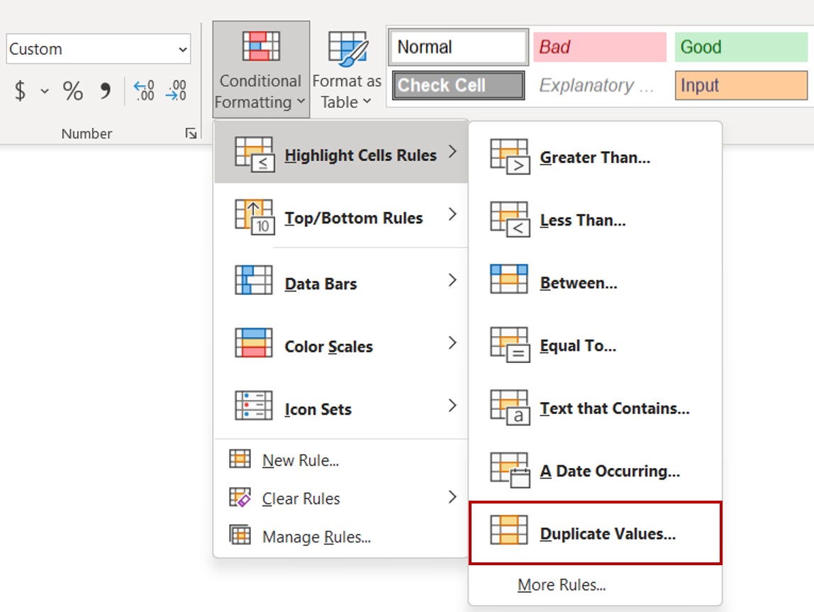
- Go to Home –> Conditional Formatting –> Highlight Cell Rules –> Duplicate Values.
- In the Duplicate Values dialog box, select Duplicate in the drop down on the left, and specify the format in which you want to highlight the duplicate values. You can choose from the ready-made format options (in the drop down on the right), or specify your own format.

- This will highlight all the values that have duplicates.

Quick Tip: Remember to check for leading or trailing spaces. For example, “John” and “John ” are considered different as the latter has an extra space character in it. A good idea would be to use the TRIM function to clean your data.
Finding and Highlight Duplicates in Multiple Columns in Excel
If you have data that spans multiple columns and you need to look for duplicates in it, the process is exactly the same as above.
Here is how to do it:
- Select the data.
- Go to Home –> Conditional Formatting –> Highlight Cell Rules –> Duplicate Values.
- In the Duplicate Values dialog box, select Duplicate in the drop down on the left, and specify the format in which you want to highlight the duplicate values.
- This will highlight all the cells that have duplicates value in the selected data set.

Finding and Highlighting Duplicate Rows in Excel
Finding duplicate data and finding duplicate rows of data are 2 different things. Have a look:
 Finding duplicate rows is a bit more complex than finding duplicate cells.
Here are the steps:
- In an adjacent column, use the following formula:
=A2&B2&C2&D2
Drag this down for all the rows. This formula combines all the cell values as a single string. (You can also use the CONCATENATE function to combine text strings)
 By doing this, we have created a single string for each row. If there are duplicate rows in this dataset, then these strings would be exactly the same for it.
Now that we have the combined strings for each row, we can use conditional formatting to highlight duplicate strings. A highlighted string implies that the row has a duplicate.
Here are the steps to highlight duplicate strings:
- Select the range that has the combined strings (E2:E16 in this example).
- Go to Home –> Conditional Formatting –> Highlight Cell Rules –> Duplicate Values.
- In the Duplicate Values dialog box, make sure Duplicate is selected and then specify the color in which you want to highlight the duplicate values.
This would highlight the duplicate values in column E.
 In the above approach, we have highlighted only the strings that we created.
But what if you want to highlight all the duplicate rows (instead of highlighting cells in one single column)?
Here are the steps to highlight duplicate rows:
- In an adjacent column, use the following formula:
=A2&B2&C2&D2
Drag this down for all the rows. This formula combines all the cell values as a single string.
- Select the data A2:D16.
- With the data selected, go to Home –> Conditional Formatting –> New Rule.

- In the ‘New Formatting Rule’ dialog box, click on ‘Use a formula to determine which cells to format’.
- In the field below, use the following COUNTIF function:
=COUNTIF($E$2:$E$16,$E2)>1
- Select the format and click OK.
This formula would highlight all the rows that have a duplicate.

Remove Duplicates in Excel
In the above section, we learned how to find and highlight duplicates in excel. In this section, I will show you how to get rid of these duplicates.
Remove Duplicates from a Single Column in Excel
If you have the data in a single column and you want to remove all the duplicates, here are the steps:
- Select the data.
- Go to Data –> Data Tools –> Remove Duplicates.

- In the Remove Duplicates dialog box:
- If your data has headers, make sure the ‘My data has headers’ option is checked.
- Make sure the column is selected (in this case there is only one column).

- Click OK.
This would remove all the duplicate values from the column, and you would have only the unique values.
CAUTION: This alters your data set by removing duplicates. Make sure you have a back-up of the original data set. If you want to extract the unique values at some other location, copy this dataset to that location and then use the above-mentioned steps. Alternatively, you can also use Advanced Filter to extract unique values to some other location.
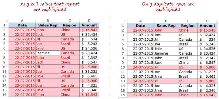
Remove Duplicates from Multiple Columns in Excel
Suppose you have the data as shown below:

In the above data, row #2 and #16 have the exact same data for Sales Rep, Region, and Amount, but different dates (same is the case with row #10 and #13). This could be an entry error where the same entry has been recorded twice with different dates.
To delete the duplicate row in this case:
- Select the data.
- Go to Data –> Data Tools –> Remove Duplicates.
- In the Remove Duplicates dialog box:
- If your data has headers, make sure the ‘My data has headers’ option is checked.
- Select all the columns except the Date column.

- Click OK.
This would remove the 2 duplicate entries.
NOTE: This keeps the first occurrence and removes all the remaining duplicate occurrences.
Remove Duplicate Rows in Excel
To delete duplicate rows, here are the steps:
- Select the entire data.
- Go to Data –> Data Tools –> Remove Duplicates.
- In the Remove Duplicates dialog box:
- If your data has headers, make sure the ‘My data has headers’ option is checked.
- Select all the columns.

- Click OK.
Use the above-mentioned techniques to clean your data and get rid of duplicates.
You May Also Like the Following Excel Tutorials:
- 10 Ways to Clean Data in Excel Spreadsheets.
- Remove Leading and Trailing Spaces in Excel.
- 24 Daily Excel Issues and their Quick Fixes.
- How to Find Merged Cells in Excel.
Highlight Duplicates (Table of Contents)
- Highlight Duplicates in Excel
- How to Highlight Duplicate Values in Excel?
- Conditional Formatting- Duplicate Values Rule
- Conditional Formatting – Using Excel Function or Custom Formula (COUNTIF)
Highlight Duplicates in Excel
We can highlight the duplicate values in the selected dataset, whether it is a column or row of a table, from Highlight Cells Rule, which is available in Conditional Formatting under the Home menu tab. To highlight the duplicates, select the data from where we need to highlight the duplicates, then select the Duplicate Values option, which is there under Conditional Formatting. From the box of Duplicate Values, choose Duplicate with the type of color formatting we want. Mostly Red text is selected by default to highlight duplicates.
There are various ways to find duplicate values in excel. They are:
- Conditional Formatting – Using Duplicate Values Rule
- Conditional Formatting – Using Excel Function or Custom Formula (COUNTIF)
How to Highlight Duplicate Values in Excel?
Highlighting Duplicate Values in Excel is very simple and easy. Let’s understand the working of finding and highlighting duplicate values in excel by using two methods.
You can download this Highlight Duplicates Excel Template here – Highlight Duplicates Excel Template
Conditional Formatting – Duplicate Values Rule
Here we will find the duplicate values in excel using the conditional formatting feature and will highlight those values. Let’s take an example to understand this process.
Example #1
We have given the below dataset.

For highlighting the duplicate values in the above dataset, follow below steps:
- Select the entire dataset.
- Go to the HOME tab.
- Click on the Conditional Formatting option under the Styles section, as shown in the below screenshot.

- It will open a drop-down list of formatting options, as shown below.
- Click on Highlight Cells Rules here, and it will again display a list of rules here. Choose the Duplicate Values option here.
- It will open a dialog box of Duplicate Values, as shown in the below screenshot.
- Select the color from the color palette for highlighting the cells.
- It will highlight all the duplicate values in the given data set. The result is shown below.
With the highlighted duplicate values, we can take action accordingly.
In the upper section, we highlighted the cells with conditional formatting inbuilt feature. We can also do this method by using an Excel function.
Conditional Formatting – Using Excel Function or Custom Formula (COUNTIF)
We will use here COUNTIF function. Let’s take an example to understand this method.
Example #2
Let’s again take the same dataset values for finding the duplicate values in excel.
For highlighting the duplicate values here, we will use the COUNTIF function here that returns TRUE if a value appears more than once in the list.
The COUNTIF function, we will use like shown below:
=COUNTIF(Cell range, Starting cell address)>1
Follow the below steps to do this.
- Select the whole dataset.
- Go to the HOME tab and click on the Conditional Formatting option.
- It will open a drop-down list of formatting options, as shown below.

- Click on the New Rule option here. Refer to the below screenshot.
- It will open a dialog box for creating a new custom rule here, as we can see below.
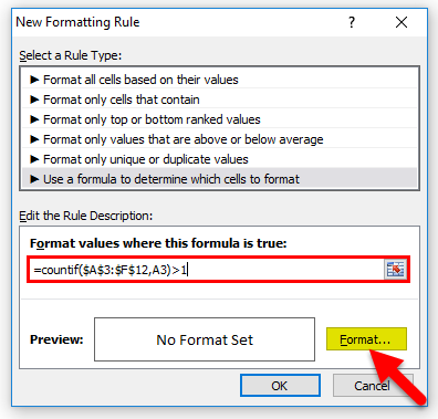
- Select the last option, “Use a formula determining which cells to format”, under the Select a Rule Type section.
- It will display a formula window, as shown below.
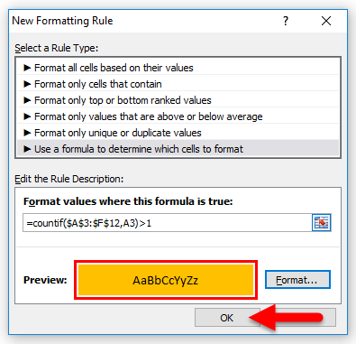
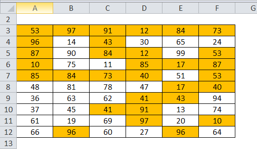
- Enter the formula as =countif($A$3:$F$12,A3)>1 then click on the Format tab.
- Choose the Fill color from the color palette for highlighting the cells, and then click on OK.
- This will highlight all the cells having duplicate values in the dataset. The result is shown below:
Things to Remember about Excel Highlight Duplicate Values
- Finding and highlighting the duplicate values in excel often comes into use while managing attendance sheets, address directories, or other related documents.
- After highlighting duplicate values, if you are deleting those records, be extra cautious about impacting your entire dataset.
Recommended Articles
This has been a guide to Highlight Duplicates in Excel. Here we discuss how to highlight duplicate values in excel by using two methods: practical examples and a downloadable excel template. You can also go through our other suggested articles –
- Goal Seek in Excel
- Tables in Excel
- Excel Combo Box
- Scrollbar in Excel
When you are working with large quantities of data, it’s easy to lose track of data and see them appear multiple times in the table. Some duplicates are placed intentionally while others are mistakes. Whatever the cases, you may want to have these duplicates automatically highlighted to you.
Finding duplicate cells in a small spreadsheet is easy but when dealing with large, complex datasets, it can be quite difficult to do it manually. Fortunately, there are built-in tools in Excel that lets you highlight duplicates values. In this tutorial, we are going to show you how to highlight duplicate data with the conditional formatting feature in Excel.
Highlight Duplicates with Conditional Formatting in Excel. Generally, you may want to find duplicates in Excel, because more than often duplicates are there by mistake and should be deleted or duplicates are important for analysis and should be highlighted in Excel.
There are two methods to find duplicate values with conditional formatting in Excel. They are:
- Highlight duplicates using the Duplicate Value rule
- Highlight duplicates using Excel custom formula (COUNTIF and COUNTIFS)
Highlight Duplicates Using Duplicate Value Rule
Let’s assume we have this data set:
First, select the range of cells that contains duplicate values. Then go to the ‘Home’ tab, click ‘Conditional Formatting’ in the Styles section of the ribbon. In the drop-down, move your cursor over the first option for ‘Highlight Cell Rules’ and it will again display a list of rules in a pop-out box. Choose the ‘Duplicate Values’ option here.
Once you click on Duplicate Values, the Duplicate Values dialogue box will appear. Here you can select the formatting type for the duplicate values. You can select from colors to only fill the cells, only for the font, as a border, or a custom format if you prefer. Then click ‘OK’ to close the dialog box.
Here, we are selecting ‘Green Fill with Dark Green Text’ for our example.
Once you select the formatting type, it will highlight all the duplicate values in the selected range as shown below.
Highlight Duplicates Using COUNTIF Formula
Another method to highlight duplicates values is to use conditional formatting with simple COUNTIF formula in a single column or across multiple columns.
Select the data range where you want to highlight the duplicates. Then on the ‘Home’ tab and click on the ‘Conditional Formatting’ option. In the drop-down, click on the ‘New Rule’ option.
This will open up a New Formatting Rule dialog box.
In the New Formatting Rule dialog box, select the ‘Use a formula to determine which cells to format’ option under the Select a Rule Type list box, then enter the following COUNTIF formula to count duplicates.
=COUNTIF($A$1:$C$11,A1)>1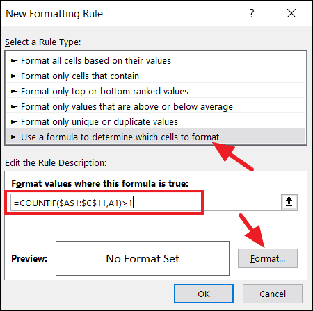
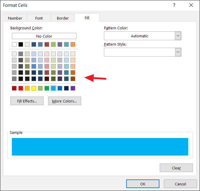
Then, click the ‘Format’ button to go to the Format Cells dialog box. In the Format Cells dialog box, you can choose the Fill color from the color palette for highlighting the cells and then click ‘OK’. Here we’re choosing blue fill color to format the duplicates.
Then, click ‘OK’ again to close the dialog box. The formula will highlight all the cell values that appear more than once.
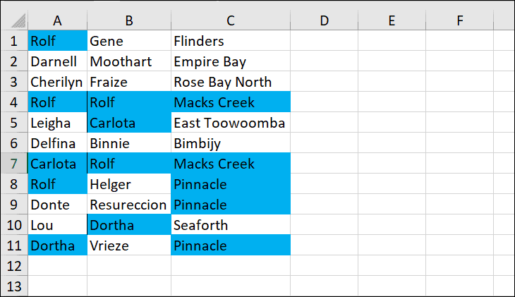
Always enter the formula for the upper-left cell in the selected range (A1:C11). Excel automatically copies the formula to the other cells.
You can also define rules however you want. For example, If you want to find values that appear only two times in a table, then enter this formula instead (In the New Formatting Rule dialog box):
=COUNTIF($A$1:$C$11,A1)=2The result:
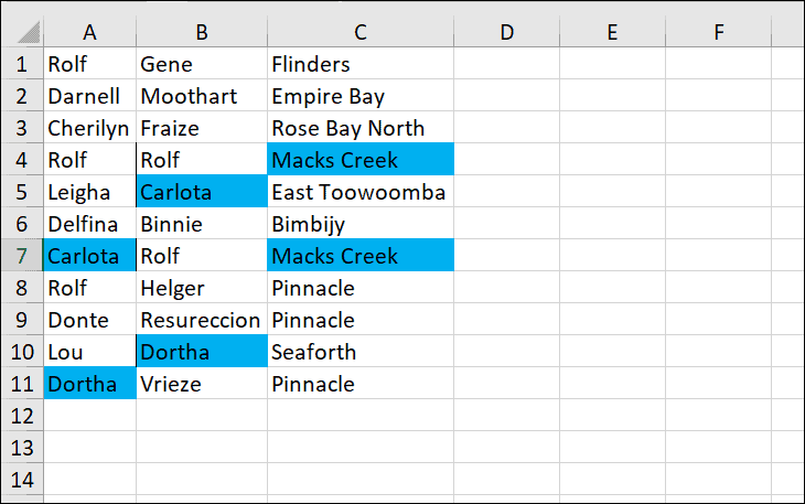
Sometimes you may want to see only the duplicates and filter out unique values. To do this, select the range, go to the Home tab, click the ‘Sort & Filter’ option at the top right corner of excel and select the ‘Filter’ option.
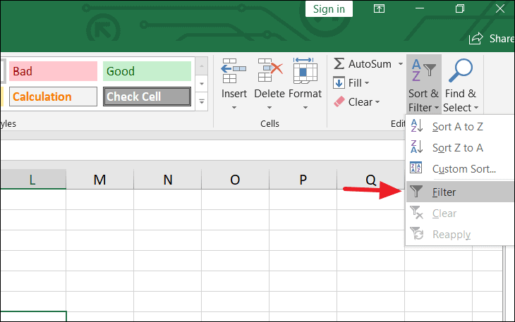
The first cell of every column will then show a drop-down menu where you can define the filter criterion. Click on the drop-down in the first cell of the column and select ‘Filter by Color’. Then choose the blue color.
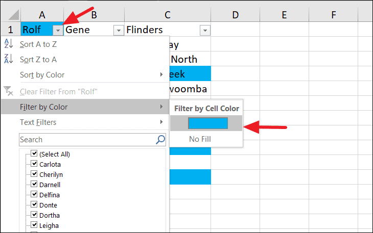
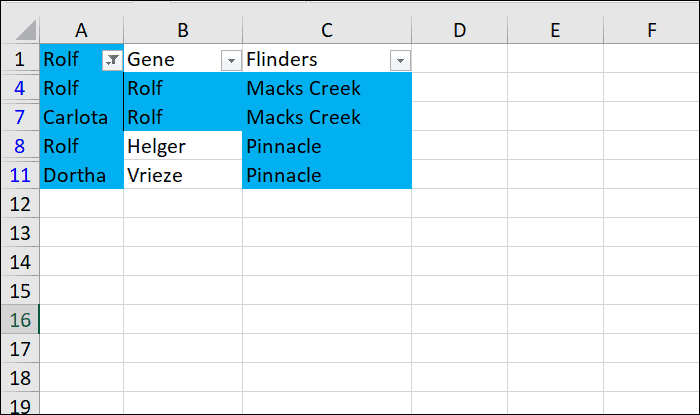
Now, you’ll see only the highlighted cells and you can do whatever you want with them.
Find and Highlight Duplicate Rows in Excel using COUNTIFS Formula
If you want to find and highlight duplicate rows in Excel, use COUNTIFS instead of COUNTIF.
Select the range, go to the ‘Home’ tab and click ‘Conditional Formatting in the Styles group. In the drop-down, click on the ‘New Rule’ option.
In the New Formatting Rule dialog box, select the ‘Use a formula to determine which cells to format’ option under the Select a Rule Type list box, then enter the below COUNTIFS formula:
=COUNTIFS($A$1:$A$20,$A1,$B$1:$B$20,$B1,$C$1:$C$20,$C1)>1In the above formula, the range A1:A20 refers to column A, B1:B20 refers to column B and C1:C20 refers to column C. The formula counts the number of rows based on multiple criteria (A1, B2, and C1).
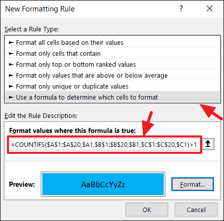
Then, click ‘Format’ button to select a formatting style and click ‘OK’.
Now, Excel highlights only the duplicate rows as shown below.
That’s it.
![]()
Find Duplicates in Excel

It is very easy to find duplicates in Excel. We can use built in tools (Conditional Formats, Filters) or formula (COUNTIF or VLOOKUP) to find duplicates in Excel Columns or Rows. Let us see the best and easy methods to find duplicate values in Excel.
Find duplicates Using Conditional Formatting
We can easily identify the duplicates using Conditional Formatting Tools in Excel. We can select the range and highlight the duplicate values with color. Following are the different methods to find duplicate entries in excel and strikethrough the duplicates using Conditional Formatting.
Highlighting duplicate values in Excel
We can highlight the duplicate values in the Excel with specific color. We can change the fill color and font color for the duplicate values. Please follow the below steps to identify the duplicates.
- Select the required range of cell to find duplicates
- Go to ‘Home’ Tab in the Ribbon Menu
- Click on the ‘Conditional Formatting’ command
- Go to ‘Highlight Cells Rules’ and Click on ‘Duplicate Values…’
- And Choose the formatting Options from the drop down list and Click on ‘OK’
Now you can see that all the duplicate values are highlighted as shown in the screen-shot.
Strike through duplicate values in Excel
We can strike through the duplicate values in the Excel. It is very helpful to strike out all duplicate entries in a range of cells. We can use the conditional formatting command in Excel to strike through the duplicate Cells.

- Select the required range of cell to strike through the duplicates
- Go to ‘Home’ Tab in the Ribbon
- Click on the ‘Conditional Formatting’ command
- Go to ‘Highlight Cells Rules’ and Click on ‘Duplicate Values…’
- And Choose the Custom Format from formatting Options from the drop down list
- Select the Strikethrough option from Font effects and Click on ‘OK’
Now you can see that all the duplicate values are stroked out as shown in the screen-shot.
Formula for checking duplicates
We can create formula using COUNTIF or VLOOKUP Functions to check the duplicates in Excel. Following is the step by explanation for finding duplicate values using Excel Formula.
Finding Duplicates using COUNTIF Formula
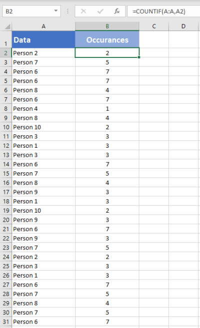
We can use COUNTIF Formula in Excel Cells to identify duplicates in Excel. COUNTIF formula helps to find duplicates in One Column, returns the number of occurrences of a given value. We can identify the duplicates if the Count is greater than 1. We can create new column to mark the duplicates using Excel COUNTIF Formula.
You can see that we have enter the COUNTIF formula in Range B2 to check the total occurrences of A1 value in the entire Column A:A.This will return the frequency of each Cell value of Column A in Column B.
We can identify the duplicate Cells based on the value in the Column B. If the values is greater than 1, we confirm that the values contains duplicate entries in the specified range or column.
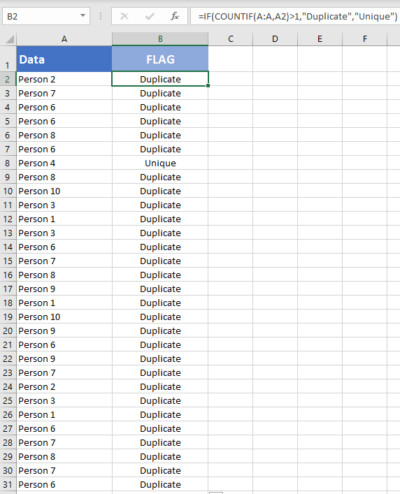
Mark Duplicates and Unique Entries using Formula
We can enhance the above formula to mark all duplicates in a Column. The following formula will return ‘Duplicate’ if the cell value contains duplicate values, otherwise returns ‘Unique’.
=IF(COUNTIF(A:A,A2)>1,"Duplicate","Unique")
Formula will return ‘Duplicate’ in the Column B if the value repeats (count >1).
It will return ‘Unique’ in the Column B if the count is 1.
Find duplicate values in excel using VLookup
We can use VLOOKUP formula to compare two columns (or lists) and find the duplicate values. Vlookup helps to find duplicates in Two Column and duplicate rows based on Multiple Columns. Following are steps to find duplicates using VLOOKUP function.
We have two lists in the Excel List 1 in Column A and List 2 in Column B. Let us find the duplicate values in the List 2 which are part of List 1.
=VLOOKUP(B2,$A$2:$A$15,1,FALSE)
VLOOKUP Formula will check for the Cell B2 value in the specified Range (A2:A5) and Returns the value if found, it will return #NA if it is not found in List 1. We can confirm if the the value is duplicated in List 1 and 2 if it returns the Value, it will be unique if it returns #NA.

How to find duplicate values in Excel using VlookUp?
You can use Excel formula to find the duplicate values in Excel by using vlookup formula as described below. You can use the Excel VlookUp to identify the duplicates in Excel.
=IF(ISNA(VLOOKUP(B2,$A$2:$A$15,1,FALSE)),"Unique","Duplicate")
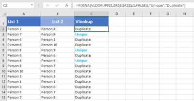
We can enhance this formula to identify the duplicates and unique values in the Column 2. We can use the Excel IF and ISNA Formulas along with VLOOKUP to return the required Labels.
You can use this method to compare with other worksheets and find duplicate values in Different Excel Sheets.
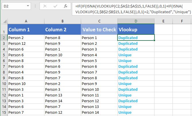
How to find duplicate values in two columns in excel using VlookUp?
Follow the below steps to find the duplicate values in two columns in excel using VlookUp. We generally need this to compare two columns and check if a value is existing in two columns.
=IF(IF(ISNA(VLOOKUP(C2,$A$2:$A$15,1,FALSE)),0,1)
+IF(ISNA(VLOOKUP(C2,$B$2:$B$15,1,FALSE)),0,1)=2,"Duplicated","Unique")
Here, we have Two Target Columns A and B , we check if the items in Column C are duplicated or not.
If you wants to compare two columns and check for values are repeated in both the columns or not, you can use this formula.
Share This Story, Choose Your Platform!
2 Comments
-
Guru
August 12, 2019 at 7:45 pm — ReplyThanks for very useful instructions to check duplicates in Excel.
-
Tom
August 12, 2019 at 7:48 pm — ReplyThis is very clear and simple! Thanks a lot for providing clear help to identify the duplicates in Excel.
© Copyright 2012 – 2020 | Excelx.com | All Rights Reserved
Page load link