
Watch Video – Highlight Rows based on Cell Values in Excel
In case you prefer reading written instruction instead, below is the tutorial.
Conditional Formatting allows you to format a cell (or a range of cells) based on the value in it.
But sometimes, instead of just getting the cell highlighted, you may want to highlight the entire row (or column) based on the value in one cell.
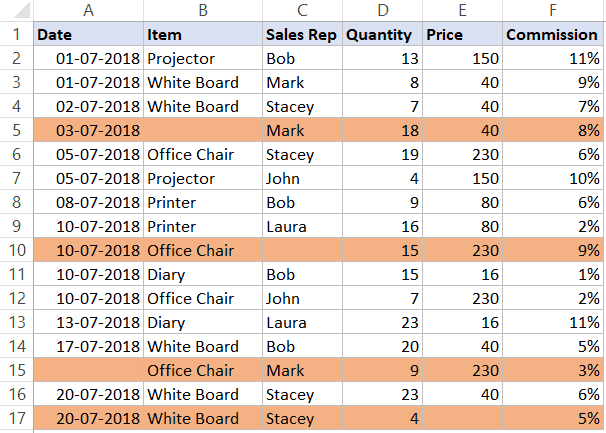
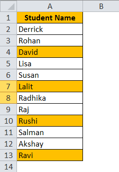
To give you an example, below I have a dataset where I have highlighted all the rows where the name of the Sales Rep is Bob.

In this tutorial, I will show you how to highlight rows based on a cell value using conditional formatting using different criteria.
Click here to download the Example file and follow along.
Highlight Rows Based on a Text Criteria
Suppose you have a dataset as shown below and you want to highlight all the records where the Sales Rep name is Bob.
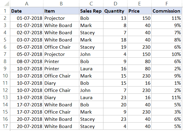
Here are the steps to do this:
- Select the entire dataset (A2:F17 in this example).
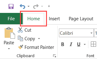
- Click the Home tab.

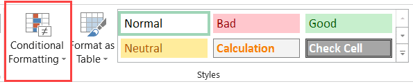
- In the Styles group, click on Conditional Formatting.

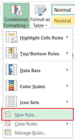
- Click on ‘New Rules’.

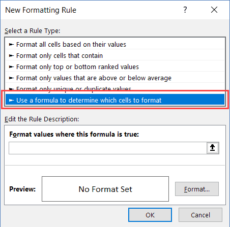
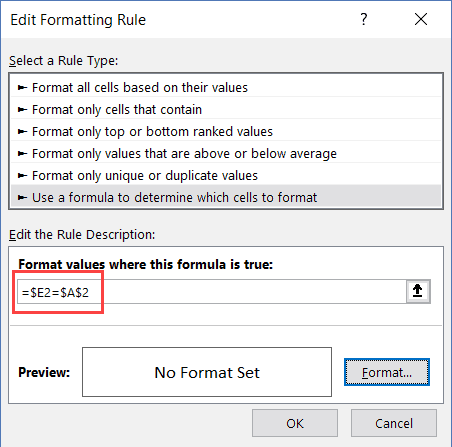
- In the ‘New Formatting Rule’ dialog box, click on ‘Use a formula to determine which cells to format’.

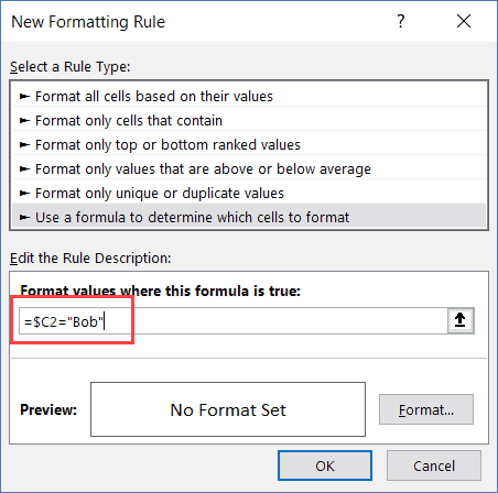
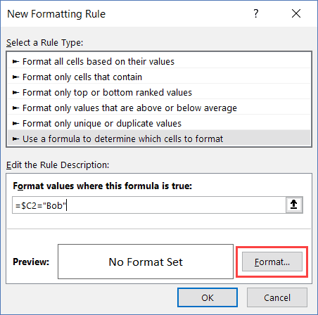
- In the formula field, enter the following formula: =$C2=”Bob”

- Click the ‘Format’ button.
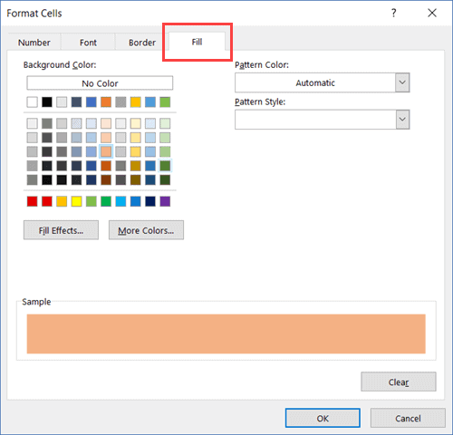
- In the dialog box that opens, set the color in which you want the row to get highlighted.

- Click OK.
This will highlight all the rows where the name of the Sales Rep is ‘Bob’.
Click here to download the Example file and follow along.
How does it Work?
Conditional Formatting checks each cell for the condition we have specified, which is =$C2=”Bob”
So when it’s analyzing each cell in row A2, it will check whether the cell C2 has the name Bob or not. If it does, that cell gets highlighted, else it doesn’t.
Note that the trick here is to use a dollar sign ($) before the column alphabet ($C1). By doing this, we have locked the column to always be C. So even when cell A2 is being checked for the formula, it will check C2, and when A3 is checked for the condition, it will check C3.
This allows us to highlight the entire row by conditional formatting.
Related: Absolute, Relative, and Mixed references in Excel.
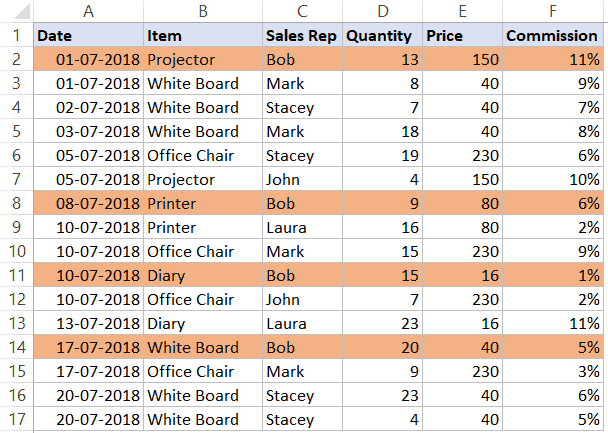
Highlight Rows Based on a Number Criteria
In the above example, we saw how to check for a name and highlight the entire row.
We can use the same method to also check for numeric values and highlight rows based on a condition.
Suppose I have the same data (as shown below), and I want to highlight all the rows where the quantity is more than 15.
Here are the steps to do this:
- Select the entire dataset (A2:F17 in this example).
- Click the Home tab.
- In the Styles group, click on Conditional Formatting.
- Click on ‘New Rules’.
- In the ‘New Formatting Rule’ dialog box, click on ‘Use a formula to determine which cells to format’.
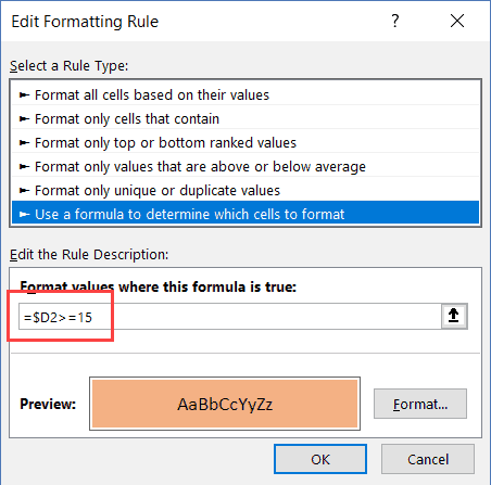
- In the formula field, enter the following formula: =$D2>=15
- Click the ‘Format’ button. In the dialog box that opens, set the color in which you want the row to get highlighted.
- Click OK.
This will highlight all the rows where the quantity is more than or equal to 15.
Similarly, we can also use this to have criteria for the date as well.
For example, if you want to highlight all the rows where the date is after 10 July 2018, you can use the below date formula:
=$A2>DATE(2018,7,10)
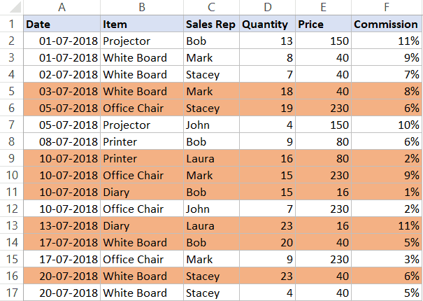
Highlight Rows Based on a Multiple Criteria (AND/OR)
You can also use multiple criteria to highlight rows using conditional formatting.
For example, if you want to highlight all the rows where the Sales Rep name is ‘Bob’ and the quantity is more than 10, you can do that using the following steps:
- Select the entire dataset (A2:F17 in this example).
- Click the Home tab.
- In the Styles group, click on Conditional Formatting.
- Click on ‘New Rules’.
- In the ‘New Formatting Rule’ dialog box, click on ‘Use a formula to determine which cells to format’.
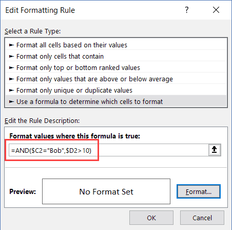
- In the formula field, enter the following formula: =AND($C2=”Bob”,$D2>10)
- Click the ‘Format’ button. In the dialog box that opens, set the color in which you want the row to get highlighted.
- Click OK.
In this example, only those rows get highlighted where both the conditions are met (this is done using the AND formula).
Similarly, you can also use the OR condition. For example, if you want to highlight rows where either the sales rep is Bob or the quantity is more than 15, you can use the below formula:
=OR($C2="Bob",$D2>15)
Click here to download the Example file and follow along.
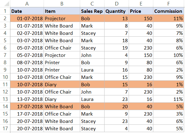
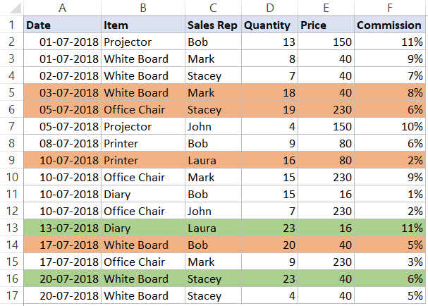
Highlight Rows in Different Color Based on Multiple Conditions
Sometimes, you may want to highlight rows in a color based on the condition.
For example, you may want to highlight all the rows where the quantity is more than 20 in green and where the quantity is more than 15 (but less than 20) in orange.
To do this, you need to create two conditional formatting rules and set the priority.
Here are the steps to do this:
- Select the entire dataset (A2:F17 in this example).
- Click the Home tab.
- In the Styles group, click on Conditional Formatting.
- Click on ‘New Rules’.
- In the ‘New Formatting Rule’ dialog box, click on ‘Use a formula to determine which cells to format’.
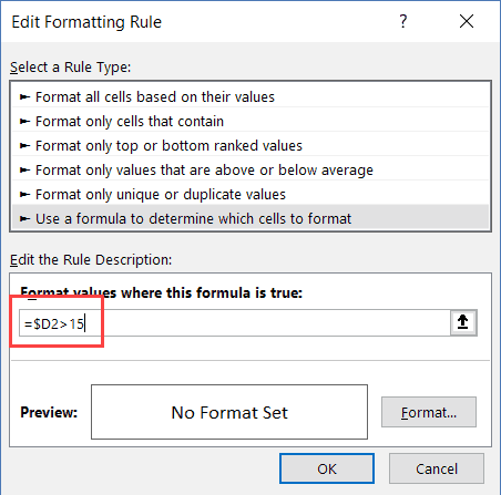
- In the formula field, enter the following formula: =$D2>15
- Click the ‘Format’ button. In the dialog box that opens, set the color to Orange.
- Click OK.
- In the ‘Conditional Formatting Rules Manager’ dialog box, click on ‘New Rule’.

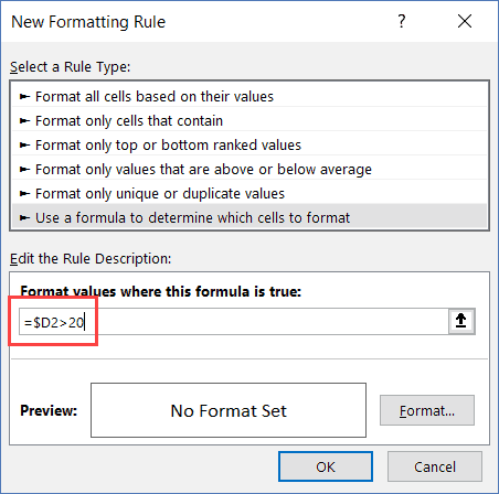
- In the ‘New Formatting Rule’ dialog box, click on ‘Use a formula to determine which cells to format’.
- In the formula field, enter the following formula: =$D2>20
- Click the ‘Format’ button. In the dialog box that opens, set the color to Green.
- Click OK.
- Click Apply (or OK).
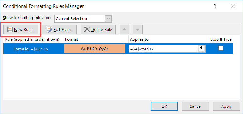
The above steps would make all the rows with quantity more than 20 in green and those with more than 15 (but less than equal to 20 in orange).
Understanding the Order of Rules:
When using multiple conditions, it important to make sure the order of the conditions is correct.
In the above example, the Green color condition is above the Orange color condition.
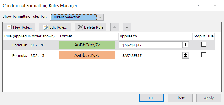
If it’s the other way round, all the rows would be colored in orange only.
Why?
Because a row where quantity is more than 20 (say 23) satisfies both our conditions (=$D2>15 and =$D2>20). And since Orange condition is at the top, it gets preference.
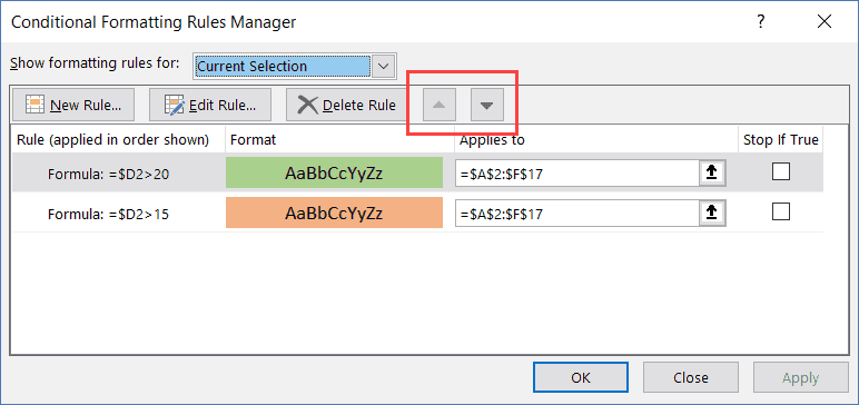
You can change the order of the conditions by using the Move Up/Down buttons.
Click here to download the Example file and follow along.
Highlight Rows Where Any Cell is Blank
If you want to highlight all rows where any of the cells in it is blank, you need to check for each cell using conditional formatting.
Here are the steps to do this:
- Select the entire dataset (A2:F17 in this example).
- Click the Home tab.
- In the Styles group, click on Conditional Formatting.
- Click on ‘New Rules’.
- In the ‘New Formatting Rule’ dialog box, click on ‘Use a formula to determine which cells to format’.
- In the formula field, enter the following formula: =COUNTIF($A2:$F2,””)>0
- Click the ‘Format’ button. In the dialog box that opens, set the color to Orange.
- Click OK.
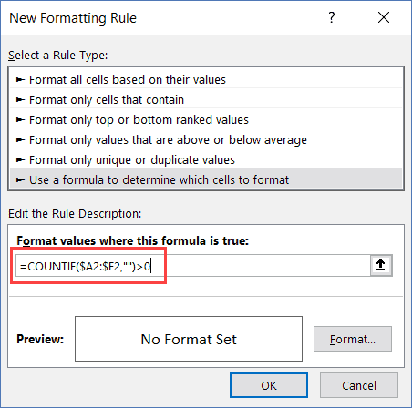
The above formula counts the number of blank cells. If the result is more than 0, it means there are blank cells in that row.
If any of the cells are empty, it highlights the entire row.
Related: Read this tutorial if you only want to highlight the blank cells.
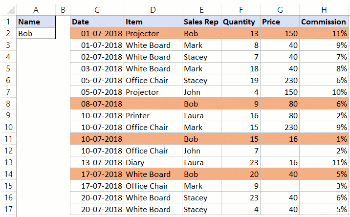
Highlight Rows Based on Drop Down Selection
In the examples covered so far, all the conditions were specified with the conditional formatting dialog box.
In this part of the tutorial, I will show you how to make it dynamic (so that you can enter the condition within a cell in Excel and it will automatically highlight the rows based on it).
Below is an example, where I select a name from the drop-down, and all the rows with that name get highlighted:
Here are the steps to create this:
- Create a drop-down list in cell A2. Here I have used the names of the sales rep to create the drop down list. Here is a detailed guide on how to create a drop-down list in Excel.
- Select the entire dataset (C2:H17 in this example).
- Click the Home tab.
- In the Styles group, click on Conditional Formatting.
- Click on ‘New Rules’.
- In the ‘New Formatting Rule’ dialog box, click on ‘Use a formula to determine which cells to format’.
- In the formula field, enter the following formula: =$E2=$A$2
- Click the ‘Format’ button. In the dialog box that opens, set the color to Orange.
- Click OK.
Now when you select any name from the drop-down, it will automatically highlight the rows where the name is the same that you have selected from the drop-down.
Interested in learning more on how to search and highlight in Excel? Check the below videos.
You May Also Like the Following Excel Tutorials:
- Dynamic Excel Filter – Extracts Data as you Type.
- Create a drop-down list with a search suggestion.
- How to Insert and Use a Checkbox in Excel.
- Select Visible Cells in Excel.
- Highlight Active Row/Column in a Data Range.
- Delete rows based on cell value in Excel
- How to Delete Every Other Row in Excel
- Apply Conditional Formatting Based on Another Column in Excel
Learn how to highlight rows in Excel with Conditional Formatting in this tutorial. We have detailed methods on highlighting rows according to text or numbers, multiple conditions, and blank cells all using Conditional Formatting. Also learn a really cool trick to highlight rows based on the value entered in a separate cell.
Conditional Formatting is an Excel feature that applies specified formatting to cells that meet the supplied criteria. Also, Conditional Formatting is dynamic; it adapts to added, deleted, and edited data. So everything you learn below will be applied to your data dynamically.
You often need values highlighted in datasets, some as a red flag and some as a green flag because they satisfy certain criteria. Since these values are the particulars of a product or person, it would help to have the full row highlighted so you don’t have to eye the highlighted cell first and then see what product or person it is about. A little explanation on how this works before we get down to the methods.
Let’s get highlighting!

Highlighting Entire Row Vs Highlighting a Cell
If you were to directly head to Highlight Cell Rules in Conditional Formatting, you would be highlighting individual cells. Let’s show you an example and explain how highlighting the row instead of just the cell works. Take this dataset as an example:

We have a list of granola bars and want to search for bars that contain eggs as an allergen. Instead of just highlighting the allergen in column C, we want the whole product highlighted which means we want to highlight the full row. Using Conditional Formatting, the rule we will set will be with this formula:
=$C3="Eggs"
Only the column is locked in reference with a dollar sign, not the row. So the formula goes row by row checking the cells starting from row 3 as mentioned in the formula. While the formula searches row by row, it checks only column C as we have entered column C as an absolute reference. When the formula finds «Eggs» in column C, it highlights the whole row. It also helps to select the entire dataset instead of just the column to have the whole rows highlighted.
Highlight Rows Based on a Text Criterion
Setting a new rule in Excel’s Conditional Formatting feature can help us highlight rows based on a text criterion. You may have a dense dataset of products and you need to find and highlight a product based on its name or some other textual quality. That is all too easy with Conditional Formatting.
Using our example, we want to find the granola bars containing the allergen eggs. We will use Conditional Formatting with a new rule to find the text «Eggs» in column C and highlight the rows. These are the steps to highlight rows based on a text criterion:
- Select the whole dataset, except the headers.

- In the Home tab’s Styles group, select the Conditional Formatting button to open its menu.
- Select New Rule… from the menu to open the New Formatting Rule window.

- Select the last rule type «Use a formula to determine which cells to format«.
- In the field provided for the formula, enter the formula:
=$C3="Eggs"
C3 is the first cell from the column containing the word you are searching for, preceded by a dollar sign $.
«Eggs» is the word you are looking for, enclosed in double-quotes.
Note that the dollar sign is used before column C to lock the search for the word only in column C.

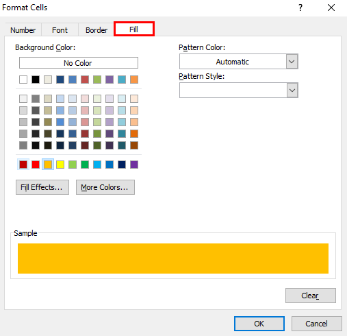
- Click on the Format… button to open the Format Cells window and then go to the Fill tab to select a color for highlighting the rows.

- Click the OK button on both windows to close them. The rows with the word «Eggs» in column C will be highlighted:

Highlight Rows Based on a Number Criterion
Using the same steps and concept as above, we can easily highlight rows based on a number criterion. Pretty much everything is the same as done earlier with a change in the formula and of course, a change in the column.
You could be looking to highlight clothing of a certain size or price, or quantities that need restocking. Extending our case example, we are aiming to highlight granola bars close to their expiry. We will show you the steps for this since formulating around a date is different than doing it for any regular number (we have a small formula example at the end of this section for simple numbers).
Below are the steps for highlighting rows based on a number criterion:
- Select all the cells in the dataset. Leave the headers out.
- Go to the Home tab > Styles group > Conditional Formatting button > New Rules… option. This leads to the New Formatting Rule window.
- In the Select a Rule Type: section, select Use a formula to determine which cells to format.
- In the Format values where this formula is true: field, enter the formula:
=$E3<DATE(2025,7,1)
E3 is the first cell from the column where the date is to be searched, a dollar sign to lock the column.
The date is entered in the format (yyyy,m,d) as required by the DATE function.
*See note below on formulas for other numbers.

- Now set the color fill for highlighting the rows by clicking on the Format…
- This redirects us to the Format Cells window.
- Go to the Fill tab and choose the color for highlighting.
- Click on the OK button on the Format Cells window and then on the New Formatting Rule

The rows with dates before 1-7-2025 in column E will be highlighted in the chosen color:

Note: Our example was based on highlighting rows falling before a certain date. If you are forming a rule based on other numeric figures such as price, quantities, etc., the formula would be quite simple. E.g. for finding granola bar prices above $1.6 in column D, the formula would be:
=$D3>1.6
Highlight Rows in Different Colors Based on Multiple Conditions
With Conditional Formatting, we will show you how to highlight rows in different colors based on multiple conditions by adding 2 rules using the Conditional Formatting Rules Manager. Each rule will have its own color and criterion.
The first criterion we will add is to search column D for values greater than 1.6. The rows containing these values will be highlighted in blue. The second rule is to highlight the rows with values greater than 1.8 in green. Now let’s see the steps for highlighting rows in different colors based on multiple conditions:
- Select the range including the dataset, excluding the headers.
- In the Home tab’s Style group, select Conditional Formatting and then select the Manage Rules… options to access the Conditional Formatting Rules Manager.

- In the Manager, select the New Rule… This will lead to the New Formatting Rule window.

- These are the 3 things you need to do in the New Formatting Rule window:
- Select the last option in the Select a Rule Type. Enter your formula in the provided field. Here’s the one we entered:
=$D3>1.6
- We are using this formula to find the values greater than 1.6 in column D, starting from the first row in the dataset which is row 3.
- Set the color for highlighting the rows that this formula applies to by clicking on the Format button then selecting the color in the Fill

- Click on the OK command button when done. You will be redirected back to the Conditional Formatting Rules Manager.
- Select the New Rule… button again to add the second rule.

- Follow the same three steps as with the first rule. Choose the last option from Select a Rule Type.
- Add your second formula. This is what we added:
=$D3>1.3
- Now we want to highlight the rows with values greater than 1.3 in column D. The first point of search is cell D3.
- Select the Format button and then the Fill tab to pick the color for highlighting the rows for the second rule.

- Click on OK. Now you will be back to the Rules Manager with both the rules added.

- Use the arrow buttons to rearrange the order of the rules. Explanation below*

- Select the OK command button.
The rows relevant to the two rules will be highlighted in the respective colors:

Note: The rule at the top gets priority and is applied before the second rule. For our case, we needed to have the first rule at the top. Had we left =$D3>1.3 at the top, all the values fulfilling the other rule =$D3>1.6 would also be greater than 1.3. That way, no row would be highlighted in blue since they have already fulfilled the criteria for the first rule.
Therefore, the rule at the top needs to be =$D3>1.6 so that the values greater than 1.6 are highlighted first and then the rest are left to be highlighted if they are greater than 1.3.
Highlight Rows Where any Cell is Blank
You may have heard of highlighting blank cells with Conditional Formatting but now we’ll show you how to highlight the whole row if any one cell in that row is blank, from any column. Not different from what we’ve seen in the methods above; we create a new rule and use a formula and color for highlighting the rows with blank cells. These are the steps to do this:
- Leaving out the headers, select the dataset.
- Go to the Home tab > Styles group > Conditional Formatting button > New Rule…
- In the New Formatting Rule window make these changes:
- Select Use a formula to determine which cells to format from the Select a Rule Type:
- Add the formula:
=COUNTBLANK($B3:$E3)>0
The COUNTBLANK function counts the number of empty cells in the range. The range included is all the columns of the dataset with the first row of the dataset. The COUNTBLANK function will count the number of blank cells in a row. If the result is greater than zero, that row will be highlighted.
- Select the color for highlighting the rows with blank cells using the Format

- Then click on OK.
The row containing a blank cell in any column will be highlighted:

Highlight Rows Based on the Value Entered in a Separate Cell
Jumping back to our first method, where we wanted to highlight the granola bars containing eggs, these were the results:
Now if you wanted to wipe out these results and highlight the rows with a dairy allergen, you would edit the formula and swap «Eggs» for «Dairy», right? How about you enter whichever allergen you want in a separate cell and it magically highlights the relevant rows?
The quick cap on that is to highlight a separate cell in the color being used for highlighting, yellow in our case. Label it for ease. Then edit the Conditional Formatting Rule from the Manager and include the separate cell in the formula instead of the value «Eggs». Then enter any allergen from column C and the rows containing the allergen will be highlighted!
Now here are the detailed steps to highlight rows based on the value entered in a separate cell:
- Use the Fill Color button to highlight a separate cell in the same color being used in the dataset.
- Also label the separate cell as we have labeled it as Allergen below:

- To open the Conditional Formatting Rules Manager, go to the Home tab > Styles group > Conditional Formatting menu > Manage Rules…

- Select the rule and click on the Edit Rule…

You will see an Edit Formatting Rule window with the current formula.

- Edit the formula: remove the value «Eggs» and replace it with the cell reference of the separate cell by clicking on it.
- The marching-ants line will appear when you click on the cell.

- Click on the OK button on both windows. Now enter a different allergen in the cell H2 and find its row highlighted:

The color fill of the separated cell doesn’t have an impact on the highlighting in the dataset but it’s used more like a key code to show what the rows with the supplied value will be highlighted in.
And that’s how we use Conditional Formatting to highlight not just cells but entire rows in Excel based on different conditions. You just need to know the formula you are working with and you’ll be good. See you with more formulas and methods that you can work well with!

Highlight Rows in Excel (Table of Contents)
- Highlight Every Other Row in Excel
- How to Highlight Every Other Row in Excel?
Highlight Every Other Row in Excel
Highlighting every other row in excel is done by the use of Conditional Formatting. This improves the readability for a user and also helps in distinguishing the different rows from other data values. Select a new rule from the Conditional Formatting list, which is under the Home menu tab, and there we can use the MOD function along with ROW to reach every second row. And then choose the color by which we want to highlight every other row in which we get the applied rule.
How to Highlight Every Other Row in Excel?
You can download this Highlight Row Excel Template here – Highlight Row Excel Template
There are various methods of highlighting or shading every other row of your data in excel.
Method 1 – Using Excel Table
This is the easiest and quickest way to highlight every other row in excel. In this method, the default ‘excel table’ option is used.
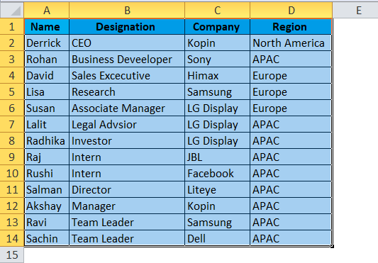
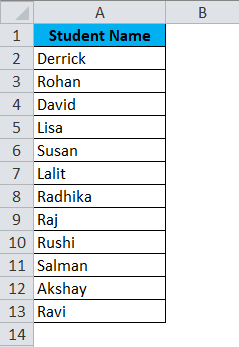
Consider the below example, where any random data is entered in the excel sheet.
The steps to highlight every other row in excel by using an excel table are as follows:
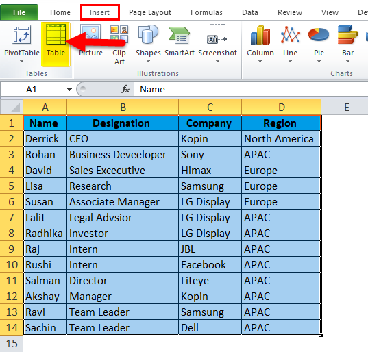
Step 1: Select the entire data entered in the excel sheet.
Step 2: From the ‘Insert’ tab, select the option ‘Table’, or else you can also press ‘Ctrl +T’, which is a shortcut to create a table.
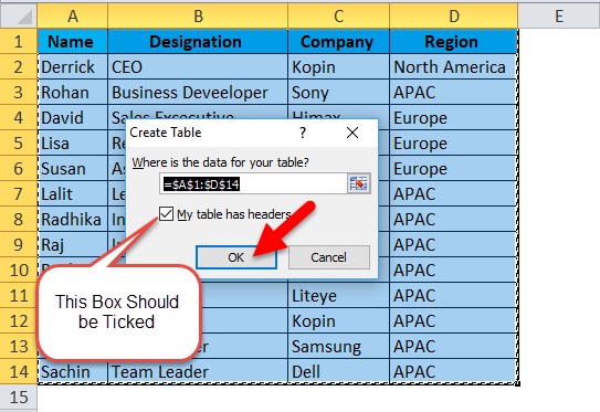
Step 3: After selecting the table option or creating the table, you will get the ‘Create Table’ dialog. In that dialog box, clicks on ‘OK’.
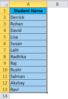
This will create a table like this.
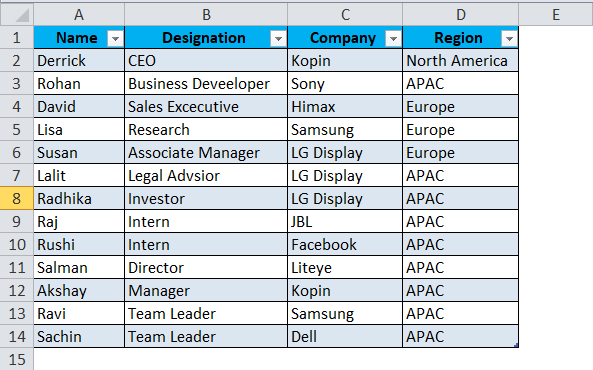
The above figure shows how every other row is highlighted.
If you want your data to look or appear in a different style or format, select the ‘Table Styles’ option from the ‘Design’ tab, as shown in the below figure.
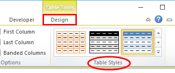
The below figure shows how modification could be done to your table by clicking the design tab, selecting the ‘Table Styles’ option, and selecting your preferred style. (Design->Table Styles)
Method 2 – Using Conditional Formatting
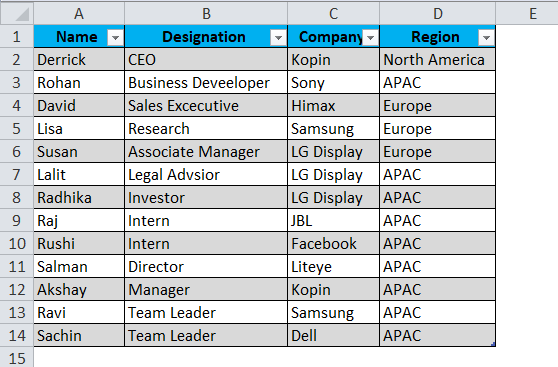
This method is useful when we want to highlight every Nth row in the spreadsheet. Consider the below example as shown in the figure.
In this example, if a teacher needs to highlight every 3rd student and group them in one group. The steps to highlight every other row in excel using conditional formatting are as follows:
Step 1: Select the data which needs to be highlighted.
Step 2: Click on ‘Home Tab’, and then click on the ‘Conditional Formatting’ icon. After clicking on conditional formatting, select the ‘New Rule’ option from the drop-down.
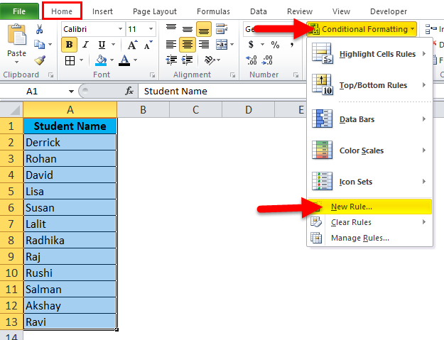
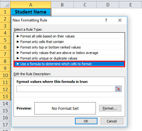
Step 3: After selecting the new rule, a dialog box will appear, from which you need to select ‘Use a formula to determine which cells to format’.
Step 4: Under the ‘Edit the Rule Description’ section, enter the formula in the empty box. Formula is ‘=MOD(ROW(),3)=1’.
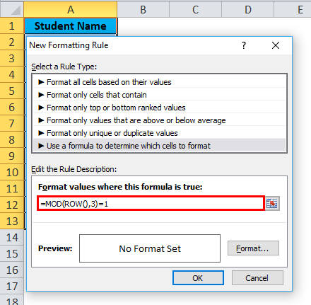
Understanding the Formula
The MOD formula returns the remainder when the ROW number is divided by 3. The formula evaluates each cell and checks if it meets the criteria. So, for example, it will check cell A3. Where the ROW number is 3, the ROW function will return 3, so the MOD function would calculate =MOD(3,3) which returns 0. But, however, this hasn’t met our designed or specified criteria. Hence, it moves to the next ROW.
Now, the cell is A4, where the ROW number is 4, and the ROW function will return 4. SO, the MOD function will calculate =MOD(4,3), and the function returns 1. This meets our specified criteria, and therefore, it highlights the entire ROW.
This formula can be customized according to your requirements. For example, consider the below modifications:
- For highlighting every 2nd ROW starting from the 1st ROW, the formula would be ‘=MOD(ROW(),2)=0’.
- To highlight every 2nd or 3rd COLUMN, the formula would be ‘MOD(COLUMN(),2)=0’ and ‘MOD(COLUMN(),3)=0’ respectively.
Step 5: After that, click on the ‘Format’ button.
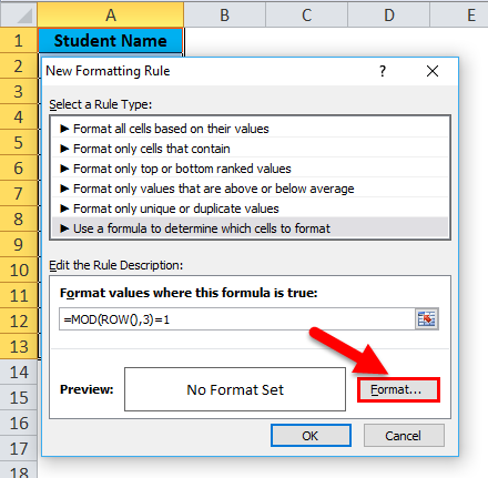
Step 6: After that, another dialog box will appear. From that, click on the ‘Fill’ tab and select any color you like.
Step 7: Click OK. This will highlight every 3rd row of our data in Excel.
Advantages
In the case of using conditional formatting, if you add new rows within range, the highlighting or shading of the alternate ROW would be done automatically.
Disadvantages
For a new user, it becomes difficult to understand the conditional formatting by using the formula for it.
Things to Remember about Highlight Every other Row in Excel
- In case you are using the excel table method or standard formatting option, and if you need to enter a new ROW within range, the shading for alternate ROW would not be done automatically. You need to do it manually.
- The MOD function can be used for ROW’s and COLUMN’s as well. You need to modify the formula accordingly.
- The color of the ROW’s cannot be changed if conditional formatting is done. You need to do follow the steps from first again.
- If a user needs to highlight both even and odd groups of ROW’s, then the user needs to create 2 conditional formattings.
- Use light colors for highlighting if the data needs to be printed.
- For Excel 2003 and below, the conditional formatting is done by first clicking on the ‘Format Menu’ and then ‘Conditional Formatting.
Recommended Articles
This has been a guide to Highlight Every Other Rows in Excel. Here we discuss how to highlight every other rows in excel using an excel table and conditional formatting along with practical examples and a downloadable excel template. You can also go through our other suggested articles –
- Add Rows in Excel Shortcut
- Autofit Row Height in Excel
- Shade Alternate Rows in Excel
- ROWS Function in Excel
Explanation
When you use a formula to apply conditional formatting, the formula is evaluated relative to the active cell in the selection at the time the rule is created. In this case, the address of the active cell (B5) is used for the row (5) and entered as a mixed address, with column D locked and the row left relative. When the rule is evaluated for each of the 40 cells in B5:E12, the row will change, but the column will not.
Effectively, this causes the rule to ignore values in columns B, C, and E and only test values in column D. When the value in column D for in a given row is «Bob», the rule will return TRUE for all cells in that row and formatting will be applied to the entire row.
Using other cells as inputs
Note that you don’t have to hard-code any values that might change into the rule. Instead you can use another cell as an «input» cell to hold the value so that you can easily change it later. For example, in this case, you could put «Bob» into cell D2 and then rewrite the formula like so:
=$D5=$D$2
You can then change D2 to any priority you like, and the conditional formatting rule will respond instantly. Just make sure you use an absolute address to keep the input cell address from changing.
Named ranges for a cleaner syntax
Another way to lock references is is to use named ranges, since named ranges are automatically absolute. For example, if you name D2 «owner», you can rewrite the formula with a cleaner syntax as follows:
=$D5=owner
This makes the formula easier to read and understand.
Excel for Microsoft 365 Excel 2021 Excel 2019 Excel 2016 Excel 2013 Excel 2010 Excel 2007 More…Less
Unlike other Microsoft Office programs, such as Word, Excel does not provide a button that you can use to highlight all or individual portions of data in a cell.
However, you can mimic highlights on a cell in a worksheet by filling the cells with a highlighting color. For a fast way to mimic a highlight, you can create a custom cell style that you can apply to fill cells with a highlighting color. Then, after you apply that cell style to highlight cells, you can quickly copy the highlighting to other cells by using Format Painter.
If you want to make specific data in a cell stand out, you can display that data in a different font color or format.
Create a cell style to highlight cells
-
Click Home > New Cell Styles.
Notes:
-
If you don’t see Cell Style, click the More
 button next to the cell style gallery.
 -
-
-
In the Style name box, type an appropriate name for the new cell style.
Tip: For example, type Highlight.
-
Click Format.
-
In the Format Cells dialog box, on the Fill tab, select the color that you want to use for the highlight, and then click OK.
-
Click OK to close the Style dialog box.
The new style will be added under Custom in the cell styles box.
-
On the worksheet, select the cells or ranges of cells that you want to highlight. How to select cells?
-
On the Home tab, in the Styles group, click the new custom cell style you created.
Note: Custom cell styles are displayed at the top of the list of cell styles. If you see the cell styles box in the Styles group, and the new cell style is one of the first six cell styles on the list, you can click that cell style directly in the Styles group.
 button next to the cell style gallery.
Use Format Painter to apply a highlight to other cells
-
Select a cell that is formatted with the highlight that you want to use.
-
On the Home tab, in the Clipboard group, double-click Format Painter
, and then drag the mouse pointer across as many cells or ranges of cells that you want to highlight. -
When you’re done, click Format Painter again or press ESC to turn it off.
 , and then drag the mouse pointer across as many cells or ranges of cells that you want to highlight.
Display specific data in a different font color or format
-
In a cell, select the data that you want to display in a different color or format.
How to select data in a cell
To select the contents of a cell
Do this
In the cell
Double-click the cell, and then drag across the contents of the cell that you want to select.
In the formula bar
Click the cell, and then drag across the contents of the cell that you want to select in the formula bar.
By using the keyboard
Press F2 to edit the cell, use the arrow keys to position the insertion point, and then press SHIFT+ARROW key to select the contents.
-
On the Home tab, in the Font group, do one of the following:
-
To change the text color, click the arrow next to Font Color
and then, under Theme Colors or Standard Colors, click the color that you want to use. -
To apply the most recently selected text color, click Font Color
. -
To apply a color other than the available theme colors and standard colors, click More Colors, and then define the color that you want to use on the Standard tab or Custom tab of the Colors dialog box.
-
To change the format, click Bold
, Italic , or Underline .Keyboard shortcut You can also press CTRL+B, CTRL+I, or CTRL+U.
-

 and then, under Theme Colors or Standard Colors, click the color that you want to use.
 , Italic
  , or Underline
  .
.Need more help?
Want more options?
Explore subscription benefits, browse training courses, learn how to secure your device, and more.
Communities help you ask and answer questions, give feedback, and hear from experts with rich knowledge.