Highlight all cells in excel

Unlike other Microsoft Office programs, such as Word, Excel does not provide a button that you can use to highlight all or individual portions of data in a cell.

However, you can mimic highlights on a cell in a worksheet by filling the cells with a highlighting color. For a fast way to mimic a highlight, you can create a custom cell style that you can apply to fill cells with a highlighting color. Then, after you apply that cell style to highlight cells, you can quickly copy the highlighting to other cells by using Format Painter.

If you want to make specific data in a cell stand out, you can display that data in a different font color or format.

Create a cell style to highlight cells

1. Click Home > New Cell Styles.

   Notes: 

   • If you don’t see Cell Style, click the More button next to the cell style gallery.

   • 

2. In the Style name box, type an appropriate name for the new cell style.

   Tip: For example, type Highlight.

3. Click Format.

4. In the Format Cells dialog box, on the Fill tab, select the color that you want to use for the highlight, and then click OK.

5. Click OK to close the Style dialog box.

   The new style will be added under Custom in the cell styles box.

6. On the worksheet, select the cells or ranges of cells that you want to highlight. How to select cells?

7. On the Home tab, in the Styles group, click the new custom cell style you created.

   Note: Custom cell styles are displayed at the top of the list of cell styles. If you see the cell styles box in the Styles group, and the new cell style is one of the first six cell styles on the list, you can click that cell style directly in the Styles group.

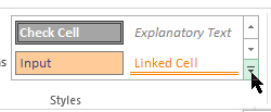
Use Format Painter to apply a highlight to other cells

1. Select a cell that is formatted with the highlight that you want to use.

2. On the Home tab, in the Clipboard group, double-click Format Painter , and then drag the mouse pointer across as many cells or ranges of cells that you want to highlight.

3. When you’re done, click Format Painter again or press ESC to turn it off.

Display specific data in a different font color or format

1. In a cell, select the data that you want to display in a different color or format.

   How to select data in a cell

   To select the contents of a cell	Do this
   In the cell	Double-click the cell, and then drag across the contents of the cell that you want to select.
   In the formula bar	Click the cell, and then drag across the contents of the cell that you want to select in the formula bar.
   By using the keyboard	Press F2 to edit the cell, use the arrow keys to position the insertion point, and then press SHIFT+ARROW key to select the contents.

2. On the Home tab, in the Font group, do one of the following:

   • To change the text color, click the arrow next to Font Color  and then, under Theme Colors or Standard Colors, click the color that you want to use.

   • To apply the most recently selected text color, click Font Color .

   • To apply a color other than the available theme colors and standard colors, click More Colors, and then define the color that you want to use on the Standard tab or Custom tab of the Colors dialog box.

   • To change the format, click Bold , Italic , or Underline .

     Keyboard shortcut  You can also press CTRL+B, CTRL+I, or CTRL+U.

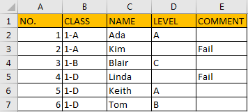
Suppose we have a table with some blank cells, if we want to highlight all non-blank cells how can we do? Though we can press ctrl and pick each non-blank cell one by one, this way is very bothersome. We need a convenient way to highlight all non-blank cells immediately. Actually, we can implement this via excel Conditional Formatting function, we can edit a new rule to filter all non-blank cells and then highlight them. We can also implement this via Go To Special function by checking on proper options. If you are familiar with VBA macro, you can also edit VBA code. This article will show you these three methods details step by step. Please read this article below and pick one of them to help you to solve your problem.

Precondition:

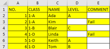
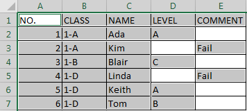
Prepare a table with some cells are blank.

We can highlight all non-blank cells via below two methods.

Method 1: Highlight All Non-Blank Cells by Conditional Formatting

---

Step 1: Select the table displayed in above screenshot.

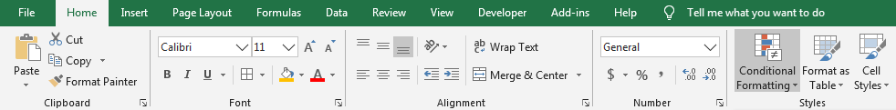
Step 2: Click Home in ribbon, click Conditional Formatting in Styles group.

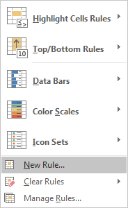
Step 3: Click the arrow on Conditional Formatting icon, select New Rule.

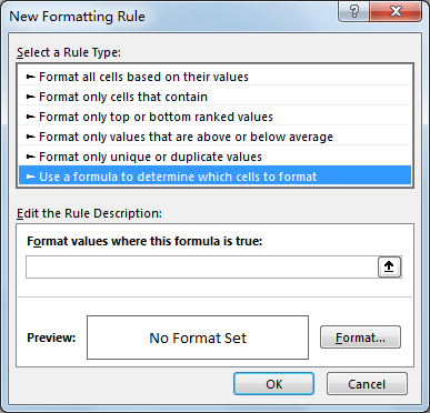
Step 4: In ‘New Formatting Rule’ dialog ‘Select a Rule Type’ pane, select ‘Use a formula to determine which cells to format’ option.

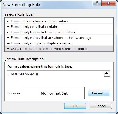
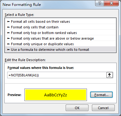
Step 5: Enter formula =NOT(ISBLANK(A1)) into ‘Format values where this formula is true.’.

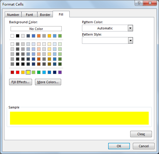
Step 6: Click Format button in Edit the Rule Description pane. On Format Cells, click Fill tab, select background color, then click OK to quit current dialog.

Step 7: In Preview field, you can see that cell is highlighted with yellow. Click OK to quit editing.

Verify that all non-blank cells are highlighted properly.

Method 2: Highlight All Non-Blank Cells by Go To Special

---

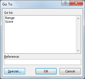
Step 1: Select the table, click F5 to load Go To dialog. Click Special button.

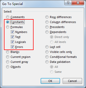
Step 2: On Go To Special dialog, check on Constants, then Numbers, Text, Logicals and Errors are activated by default. Click OK.

Step 3: After step#2, all non-blank cells are selected.

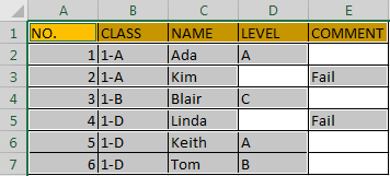
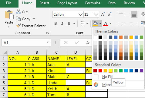
In Home ribbon, click Fill Color arrow in Font group. Select color, then non-blank cells are filled with this color.

Method 3: Highlight All Non-Blank Cells by VBA Code

---

Step 1: On current visible worksheet, right click on sheet name tab to load Sheet management menu. Select View Code, Microsoft Visual Basic for Applications window pops up.

Or you can enter Microsoft Visual Basic for Applications window via Developer->Visual Basic. You can also press Alt + F11 keys simultaneously to open it.

Step 2: In Microsoft Visual Basic for Applications window, enter below code:

Sub HighlightAllNonBlankCells()
    
    Dim myRange As Range
    Dim myCell As Range
    Dim nonEmptyCells As Range
    Set myRange = Application.ActiveSheet.UsedRange
    
    For Each myCell In myRange
        If Not (myCell.Value = "") Then
           If nonEmptyCells Is Nothing Then
              Set nonEmptyCells = myCell
           Else
              Set nonEmptyCells = Application.Union(nonEmptyCells, myCell)
           End If
        End If
    Next
    
    If Not (nonEmptyCells Is Nothing) Then
       nonEmptyCells.Select
    End If
    
End Sub

Step 3: Save code, quit Microsoft Visual Basic for Applications.

Step 4: Click Developer->Macros to run Macro.

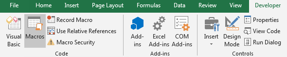
Step 5: Select ‘HighlightAllNonBlankCells’ and click Run.

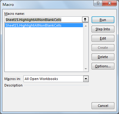
Verify that all non-blank cells are selected. Then you can follow step#3 in method#2 to fill highlight color.

Colorize your data for maximum impact

Updated on November 11, 2021

What to Know

• To highlight: Select a cell or group of cells > Home > Cell Styles, and select the color to use as the highlight.
• To highlight text: Select the text > Font Color and choose a color.
• To create a highlight style: Home > Cell Styles > New Cell Style. Enter a name, select Format > Fill, choose color > OK.

This article explains how to highlight in Excel. Additional instructions cover how to create a customized highlight style. Instructions apply to Excel 2019, 2016, and Excel for Microsoft 365.

Why Highlight?

Choosing to highlight cells in Excel can be a great way to make sure data or words stand out or increase readability within a file with a lot of information. You can select both cells and text as a highlight in Excel, and you can also customize the colors to suit your needs. Here’s how to highlight in Excel.

How to Highlight Cells in Excel

Spreadsheet cells are the boxes that contain text within a Microsoft Excel document, though many are also completely empty. Both empty and filled Excel cells can be customized in a variety of different ways, including being given a colored highlight.

1. Open the Microsoft Excel document on your device.

2. Select a cell you want to highlight.

   To select a group of cells in Excel, select one, press Shift, then select another. Alternatively, you can select individual cells that are separate from each other by holding down Ctrl while you select them.

3. From the top menu, select Home, followed by Cell Styles.

4. A menu with a variety of cell color options pops up. Hover your mouse cursor over each color to see a live preview of the cell color change in the Excel file.

5. When you find a highlight color that you like, select it to apply the change.

   If you change your mind, press Ctrl+Z to undo the cell highlight.

6. Repeat for any other cells that you want to apply a highlight to.

   To select all of the cells in a column or row, select the numbers on the side of the document or the letters at the top.

How to Highlight Text in Excel

If you just want to highlight text in Excel instead of the entire cell, you can do that too. Here’s how to highlight in Excel when you just want to change the color of the words in the cell.

1. Open your Microsoft Excel document.

2. Double-click the cell containing text you want to format.

3. Press the left mouse button and drag it across the words you want to colorize to highlight them. A small menu appears.

4. Select the Font Color icon in the small menu to use the default color option or select the arrow next to it to choose a custom color.

   You can also use this menu to apply bold or italics style options as you would in Microsoft Word and other text editor programs.

5. Select a text color from the pop-up color palette.

6. The color is applied to the selected text. Select elsewhere in the Excel document to deselect the cell.

How to Create a Microsoft Excel Highlight Style

There are a lot of default cell style options in Microsoft Excel. However, if you don’t like any of the available choices, you can create your own personal style.

1. Open a Microsoft Excel document.

2. Select Home, followed by Cell Styles.

3. Select New Cell Style.

4. Enter a name for the new cell style and then select Format.

5. Select Fill in the Format Cells window.

6. Choose a fill color from the palette. Choose the Alignment, Font or Border tabs to make other changes to the new style and then select OK to save it.

   You should now see your custom cell style at the top of the Cell Styles menu. 

Thanks for letting us know!

Get the Latest Tech News Delivered Every Day

Subscribe

Whenever you are auditing an Excel worksheet and need to know where all the formulas are located, a great way is to highlight the formula cells in a distinctive color.  This is how it is done:

STEP 1: Select all the cells in your Excel worksheet by clicking on the top left hand corner of your worksheet.

STEP 2: Press the CTRL+G shortcut which will open up the Go To dialogue box and select the Special button.

STEP 3: Select the Formula radio button and press OK.

STEP 4: This will highlight all the formulas in your Excel worksheet and you can use the Fill Color to color in the formula cells.

And now all your cells containing formulas are now highlighted!

You can practice this cool trick by downloading this workbook:

How to Highlight All Formula Cells in Excel

About The Author

Watch Video – Search and Highlight Data Using Conditional Formatting

If you work with large datasets, there can be a need to create a search functionality that allows you to quickly highlight cells/rows for the searched term.

While there is no direct way to do this in Excel, you can create search functionality using Conditional Formatting.

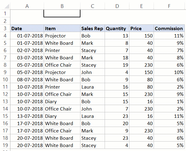
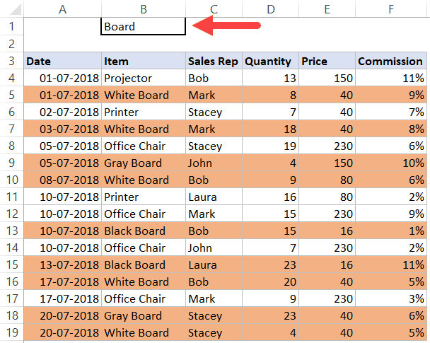
For example, suppose you have a dataset as shown below (in the image). It has columns for Product Name, Sales Rep, and Country.

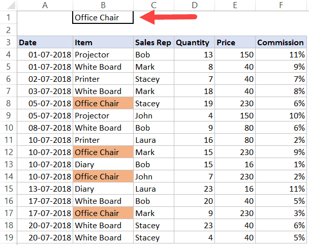
Now you can use conditional formatting to search for a keyword (by entering it in cell C2) and highlight all the cells that have that keyword.

Something as shown below (where I enter the item name in cell B2 and press Enter, the entire row gets highlighted):

In this tutorial, I will show you how to create this search and highlight functionality in Excel.

Later in the tutorial, we will go a bit advanced and see how to make it dynamic (so that it highlights while you’re typing in the search box).

Click here to download the example file and follow along.

Search and Highlight Matching Cells

In this section. I will show you how to search and highlight only the matching cells in a dataset.

Something as shown below:

Here are the steps to search and highlight all the cells that have the matching text:

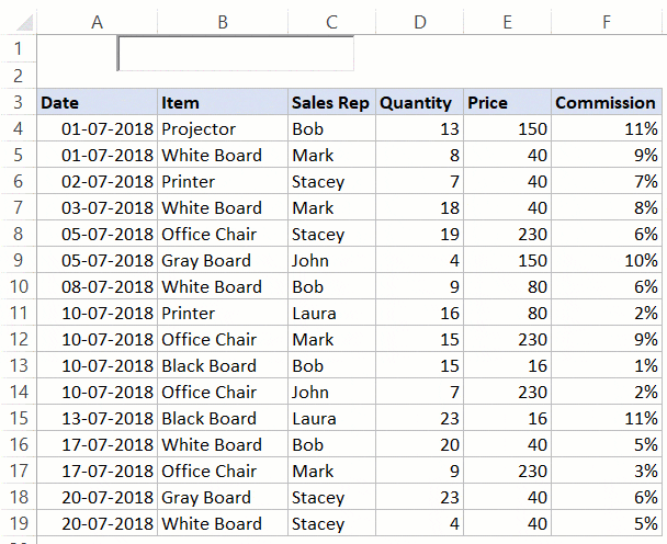
1. Select the dataset on which you want to apply Conditional Formatting (A4:F19 in this example).
2. Click the Home tab.
3. In the Styles group, click on Conditional Formatting.
4. In the drop-down options, click on New Rule.
   
5. In the ‘New Formatting Rule’ dialog box, click on the option ‘Use a formula to determine which cells to format’.
6. Enter the following formula: =A4=$B$1
7. Click on ‘Format..’ button.
8. Specify the formatting (to highlight cells that match the searched keyword).
9. Click OK.

Now type anything in cell B1 and press enter. It will highlight the matching cells in the dataset that contain the keyword in B1.

How does this work?

Conditional Formatting gets applied whenever the formula specified in it returns TRUE.

In the above example, we check each cell using the formula =A4=$B$1

Conditional Formatting checks each cell and verifies it the content in the cell is the same as that in cell B1. If it’s the same, the formula returns TRUE and the cell gets highlighted. If it isn’t the same, the formula returns FALSE and nothing happens.

Click here to download the example file and follow along.

Search and Highlight Rows with Matching Data

If you want to highlight the entire row instead of just the matching cells, you can do that by tweaking the formula a little.

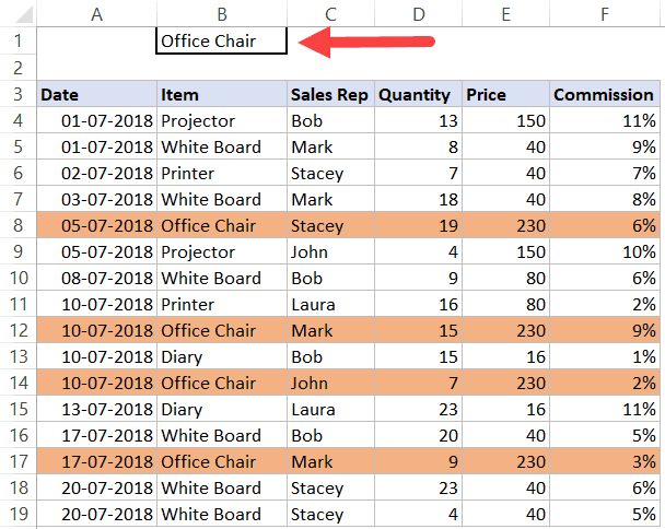
Below is an example where the entire row gets highlighted if the product type matches the one in cell B1.

Here are the steps to search and highlight the entire row:

1. Select the dataset on which you want to apply Conditional Formatting (A4:F19 in this example).
2. Click the Home tab.
3. In the Styles group, click on Conditional Formatting.
4. In the drop-down options, click on New Rule.
   
5. In the ‘New Formatting Rule’ dialog box, click on the option ‘Use a formula to determine which cells to format’.
6. Enter the following formula: =$B4=$B$1
7. Click on ‘Format..’ button.
8. Specify the formatting (to highlight cells that match the searched keyword).
9. Click OK.

The above steps would search for the specified item in the dataset, and if it finds the matching item, it will highlight the entire row.

Note that this will only check for the item column. If you enter a Sales Rep name here, it will not work. If you want it to work for Sales Rep name, you need to change the formula to =$C4=$B$1

Note: The reason it highlights the entire row and not just the matching cell is that we have used a $ sign before the column reference ($B4). Now when conditional formatting analyzes cells in a row, it checks whether the value in column B of that row is equal to the value in cell B1. So even when it’s analyzing A4 or B4 or C4 and so on, it’s checking for B4 value only (as we have locked column B by using the dollar sign).

You can read more about absolute, relative and mixed references here.

Search and Highlight Rows (based on Partial Match)

In some cases, you may want to highlight rows based on a partial match.

For example, if you have items such as White Board, Green Board, and Gray Board, and you want to highlight all these based on the word Board, then you can do this using the SEARCH function.

Something as shown below:

Here are the steps to do this:

1. Select the dataset on which you want to apply Conditional Formatting (A4:F19 in this example).
2. Click the Home tab.
3. In the Styles group, click on Conditional Formatting.
4. In the drop-down options, click on New Rule.
   
5. In the ‘New Formatting Rule’ dialog box, click on the option ‘Use a formula to determine which cells to format’.
6. Enter the following formula: =AND($B$1<>””,ISNUMBER(SEARCH($B$1,$B4)))
7. Click on ‘Format..’ button.
8. Specify the formatting (to highlight cells that match the searched keyword).
9. Click OK.

How does this work?

• SEARCH function looks for the search string/keyword in all the cells in a row. It returns an error if the search keyword is not found, and returns a number if it finds a match.
• ISNUMBER function converts the error into FALSE and the numeric values into TRUE.
• AND function checks for an additional condition – that cell C2 should not be empty.

So now, whenever you type a keyword in cell B1 and press Enter, it highlights all the rows that have the cells that contain that keyword.

Bonus Tip: If you want to make the search case sensitive, use the FIND Function instead of SEARCH.

Click here to download the example file and follow along.

Dynamic Search and Highlight Functionality (Highlights as you type)

Using the same Conditional Formatting tricks covered above, you can also take it a step further and make it dynamic.

For example, you can create a search bar where the matching data gets highlighted as you’re typing in the search bar.

Something as shown below:

This can be done using ActiveX controls and can be a good functionality to use when creating reports or dashboards.

Below is a video where I show how to create this:

Did you find this tutorial useful? Let me know your thoughts in the comments section.

You May Also Like the Following Excel Tutorials:

• Dynamic Excel Filter – Extracts Data as you Type.
• Create a drop-down list with search suggestion.
• Creating a Heat Map in Excel.
• Highlight Rows Based on a Cell Value in Excel.
• Highlight the Active Row and Column in a Data Range in Excel.
• How to Highlight Blank Cells in Excel.