Highest lowest in excel - Word и Excel - помощь в работе с программами

Excel for Microsoft 365 Excel 2021 Excel 2019 Excel 2016 Excel 2013 Excel 2010 Excel 2007 More…Less

Let’s say you want to find out who has the the smallest error rate in a production run at a factory or the largest salary in your department. There are several ways to calculate the smallest or largest number in a range.

If the cells are in a contiguous row or column

Select a cell below or to the right of the numbers for which you want to find the smallest number.
On the Home tab, in the Editing group, click the arrow next to AutoSum , click Min (calculates the smallest) or Max (calculates the largest), and then press ENTER.

If the cells are not in a contiguous row or column

To do this task, use the MIN, MAX, SMALL, or LARGE functions.

Example

Copy the following data to a blank worksheet.


1
2
3
4
5
6
7

A
Data
10
7
9
27
0
4
Formula	Description (Result)
=MIN(A2:A7)	Smallest number in the range (0)
=MAX(A2:A7)	Largest number in the range (27)
=SMALL(A2:A7, 2)	Second smallest number in the range (4)
=LARGE(A2:A7,3)	Third largest number in the range (9)

Need more help?

You can always ask an expert in the Excel Tech Community or get support in the Answers community.

Find the top 10 values in an Excel range without sorting

Select the range in column B containing Sales data for each person named in column A.
Click in the Name box in the Formatting toolbar and enter SalesData.
Enter the following formula in a cell outside the named range (for example, D2):
Press [Ctrl][Shift][Enter]

How do I rank by criteria in Excel?

Rank in Excel Using Multiple Criteria

Go to cell D2 and select it with your mouse.
Apply the formula =RANK. EQ($B2,$B$2:$B$8)+COUNTIFS($B$2:$B$8,$B2,$C$2:$C$8,”>”&$C2) to cell D2.
Press Enter.
Drag the formula to the cells below.

How do you rank content?

Here are the ten steps to rank for a keyword in Google.

Step 1: Lay the Groundwork.
Step 2: Do Your Initial Keyword Research.
Step 3: Check Out the Competition.
Step 4: Consider Intent.
Step 5: Conceptualize the Content.
Step 6: Execute.
Step 7: Optimize for Your Keyword.
Step 8: Publish.

How do I find my rank?

Therefore, to find the rank of a matrix, we simply transform the matrix to its row echelon form and count the number of non-zero rows. Consider matrix A and its row echelon matrix, A_ref.

How do you get top 5 in Excel?

Using an Array Formula to Display Top Five Values

Select cells E3 to E7. This set of cells will hold the top five client balances.
In the formula bar, enter the following formula: =LARGE(C3:C17,{1;2;3;4;5}
Then press Ctrl+Shift+Enter.
The top five balances will be displayed.

How do you find 5 highest values in Excel?

Select cell B2, copy and paste formula =LARGE(A$2:A$16,ROWS(B$2:B2)) into the formula bar, then press the Enter key. See screenshot: 2. Select cell B2, drag the fill handle down to cell B6, then the five highest values are showing.

How do you get top 3 in Excel?

Use the =LARGE(array,k) function to return the largest, second-largest, third-largest and kth largest values from a range. To set up the formulas, first build a helper column with the numbers 1, 2 and 3, as shown in K6:K8 in Figure 3.

What is easy to rank keywords?

In addition to looking at the paid difficulty number, you’ll want to find keywords that have a low SEO difficulty score. When a keyword meets those 2 requirements it means it is easy to rank and people find it valuable enough to buy ads on the keyword.

What is the fastest way to rank a keyword?

Here are 7 strategies to help you get lucky with your ranking quickly:

Use the less popular version of a keyword.
Use many keyword modifiers.
Mix up your on page optimization.
Go deeper than the competition is going.
Move away from the commercial keywords.
Buy traffic.

How do I increase my keyword ranking?

How to Improve Your Keyword Rankings in Google

Measure Your Rankings.
Target the Right Keywords.
Fix Technical Issues.
Focus on the User Experience.
Optimize for Users & Search Engines.
Create Eye-Catching & Engaging Titles.
Stay on Top of Algorithm Updates.
Provide Answers to the Questions People Are Asking.

How do you copy a rank in Excel?

If you want to rank range numbers uniquely in ascending order, please do as follows. 1. Select cell B2, copy and paste formula =RANK(A2,$A$2:$A$11,1)+COUNTIF($A$2:A2,A2)-1 into the Formula Bar, then press the Enter key. Then the first ranking number is displayed in cell B2.

What is rank of a determinant?

The “rank” of a matrix , R K ( ) , is the number of rows or columns, , of the largest × square submatrix of for which the determinant is nonzero.

What is the rank of a 3×3 matrix?

As you can see that the determinants of 3 x 3 sub matrices are not equal to zero, therefore we can say that the matrix has the rank of 3.

How do I find the lowest value in a range in Excel?

Calculate the smallest or largest number in a range

Select a cell below or to the right of the numbers for which you want to find the smallest number.
On the Home tab, in the Editing group, click the arrow next to AutoSum. , click Min (calculates the smallest) or Max (calculates the largest), and then press ENTER.

How do I find Top 5 names in Excel?

1. Finding the Top 5 Values & Names without Duplicates

1.1 Getting Top 5 Values by Using LARGE & ROWS Functions Together.
1.2 Pulling Out the Top 5 Names by Combining INDEX & MATCH Functions.
1.3 Extracting the Top 5 Names by Using XLOOKUP Function.
1.4 Finding the Top 5 Names & Values under Multiple Criteria.

Источник

If you want to find the position of a cell in the defined list of cells, you should use Excel RANK lowest to highest function. This function allows you to determine the position of a certain number in number arrays. In this tutorial, you will see how to rank chosen cell, how to get unique or average rank and how to rank number based on multiple conditions. All of these are useful functions in daily Excel usage.

Using the RANK Function in Excel

There are several ways to use rank figures in Excel and combine other function with the RANK function.

Basic RANK Function
EQ Function
AVG Function
Rank based on multiple conditions

Basic RANK Function

If you need to rank the position of the certain cell in the selected array of number cells, you should use the RANK function. It returns the position of the chosen number in the list of cells. The syntax of the function looks like:

=NUMBER(Number, Ref, [order])

The number is the cell for which we want to find the position in a list. Ref is the list of numbers (cells) in which we are determining the position of the chosen cell. The order is a non-mandatory parameter of the function and allows us to decide if we want to get a position from ascending or descending sorted list. If we put “0”, that means descending, and “1” means ascending. If this parameter is omitted, the default value is “0” – descending order. Let’s now look at one example of basic usage of RANK function:

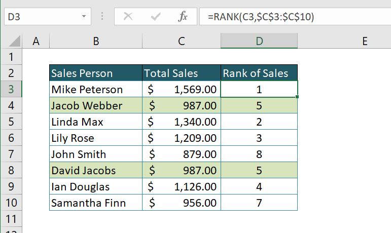
=RANK(C3,$C$3:$C$10)

In this example, we want to find the position of Salesperson based on his/her sales volume. Our number will be cell C3 and Ref (list of numbers) C3:C10 (Be sure to put “$” or press F4 button in this range, because the function will be copied to all rows). In this case, we omitted the Order parameter, which means that we want a descending order. The result is rank number one for the first cell (C3) – which is the greatest sale in this list.

EQ Function

In previous example all values of sales in our list were different, so we returned unique ranks for all rows. It can often happen that we have two or more identical numbers in the list. In this case, the RANK function will assign the same rank to all the same numbers. If we want to have unique ranks for all cells in the list, we need to use functions RANK.EQ in combination with COUNTIF function. RANK.EQ has the same syntax as the RANK function, but in case of same numbers in a list, it will assign the unique rank to all of them. First, we will look at the result of the RANK function with two of the same values in the list:

As you can see, cells C4 and C8 have identical values ($987.00), and they both got ranked 5. Next number in ranking, cell 10 has ranking 7, so rank 6 is skipped. Here is the example of using functions RANK.EQ and COUNTIF to get unique ranks:

=RANK.EQ(C3,$C$3:$C$10)+COUNTIF($C$3:C3,C3)-1

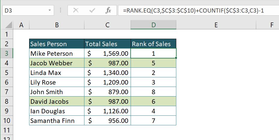
We are omitting the barrier of rank function by using COUNTIF function. Easily explained, whenever ranking value appears once, the COUNTIF function result is zero, and the formula is equal to RANK.EQ function.

For same ranking values, COUNTIF function adds zero for first multiplied value in the range. For the second same value in the range, the COUNTIF function will give you a result in 1, adding 1 on the RANK.EQ function result.

RANK.AVG Function

You can also use the RANK.AVG function, for ranking values in certain cell ranges. The only difference from the RANK/RANK.EQ functions are the treatment of equal values in a range. For the same values in the range, this function will give you the average value of the range.

Let’s look in the example below to make the situation more clear:

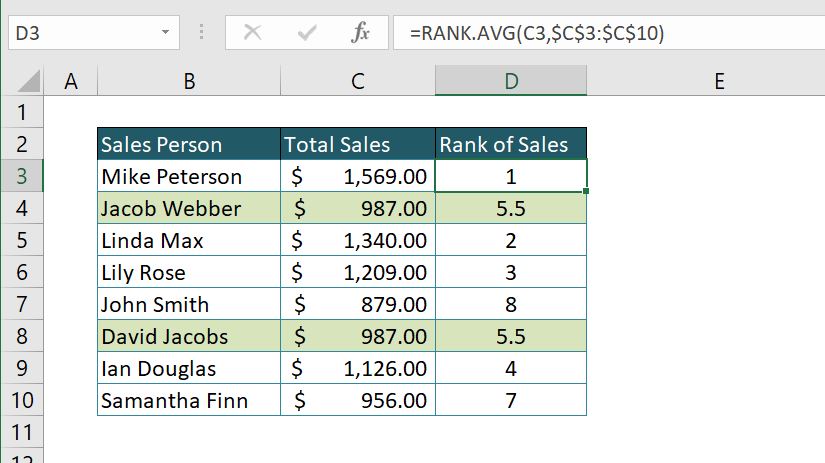
As we can see, the ranking result for the same values is 5.5, an average of 5 and 6 ranking position. In the background, a formula is assigning 5 to the first equal value, and 6 to the second, calculating average of these two numbers.

Rank based on multiple conditions

If you want to rank your data based on two or more conditions (columns), you can do it using the combination of RANK.EQ and SUMIFS function. In this way, if the values of the first column are equal, a function will look at the second column and rank based on these values. Here is the example of this case:

=RANK.EQ($C3,$C$3:$C$10)+COUNTIFS($C$3:$C$10,$C3,$D$3:$D$10,">"&$D3)

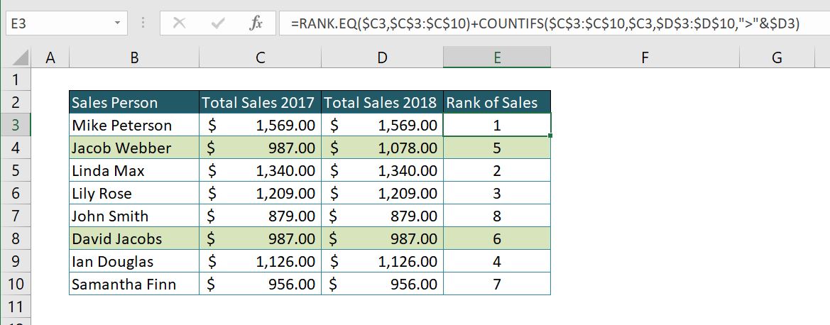
In this example, we want ranking first for Total sales in 2017, and if there are two same amounts, we want to rank based on Total sales 2018 values. Similarly to unique rank, function COUNTIFS will look at columns C and D this time, and return 1 if there is one greater value in Column D (Total values 2018). In our example, we have Jacob Webber and David Jacobs who have the same sales in 2017 ($987), but in 2018 Jacob has $1,078 and is ranked better than David who has $987.

Still need some help with Excel formatting or have other questions about Excel? Connect with a live Excel expert here for some 1 on 1 help. Your first session is always free.

Источник

As shown in the example above, to rank numbers from highest to lowest, use one of the Excel ranking formulas with the order argument set to 0 or omitted (the default). To sort a number against other numbers in ascending order, enter 1 or another non-zero value in the optional third argument. To find the position of a cell in the defined cell list, you should use the Excel RANK from lowest to highest value function. You can use this function to determine the position of a specific number in number fields.

In this tutorial, you’ll learn how to rank a selected cell, how to get a unique or average rank, and how to rank the count based on multiple conditions. All of these are useful functions in daily Excel use. If you use a zero as the order setting, or if you don’t use the third argument, the rank is set in descending order. If the order is a non-zero value, Microsoft Excel arranges the number as if the reference were a list sorted in ascending order.

The EXCEL RANK function returns the rank of a numeric value when it is compared to a list of other numeric values. After you calculate the decimal tie amounts, you can add the RANK results to the tiebreak results to obtain the final ranking. There are several ways to use rank numbers in Excel and combine other functions with the RANK function. Easy to explain, once the rank value is displayed, the result of the COUNTIF function is zero and the formula corresponds to RANK.

The EXCEL RANK function assigns a rank to a numeric value when it is compared to a list of other numeric values. Instead of using the RANK function to compare a number against a whole list of numbers, you may need to place a value within a specific subset of numbers. The tie break formula uses COUNTIF and RANK functions wrapped with an IF function to check whether a decimal tie value should be added to the original rank. If you need to order the position of a specific cell in the selected array of number cells, you should use the RANK function.

If you want to rank your data based on two or more conditions (columns), you can do so by combining RANK. If you give the RANK function a number and a list of numbers, the rank of that number appears in the list in either ascending or descending order. The EQ has the same syntax as the RANK function, but in the case of the same numbers in a list, they are all assigned the unique rank.

Malo Treille

Wannabe pop culture expert. Avid burrito trailblazer. Amateur zombie trailblazer. Avid social media nerd. Professional music advocate. Incurable tv fanatic.

Источник

If the cells are in a contiguous row or column

If the cells are not in a contiguous row or column

Example

Need more help?

See Also

Need more help?

Want more options?

Find out the highest or lowest value in a selection with formulas

To get the largest or smallest number in a range:

To get the largest 3 or smallest 3 numbers in a range:

Find and highlight the highest or lowest value in a selection with Conditional Formatting

Select all of the highest or lowest value in a selection with a powerful feature

Select the highest or lowest value in each row or column with a powerful feature

More relative largest or smallest value articles:

The Best Office Productivity Tools

Kutools for Excel Solves Most of Your Problems, and Increases Your Productivity by 80%

Office Tab Brings Tabbed interface to Office, and Make Your Work Much Easier

How do you numerically rank in Excel?

How do I sort by rank in Excel?

How do I rank up top 10 in Excel?

How do I rank by criteria in Excel?

How do you rank content?

How do I find my rank?

How do you get top 5 in Excel?

How do you find 5 highest values in Excel?

How do you get top 3 in Excel?

What is easy to rank keywords?

What is the fastest way to rank a keyword?

How do I increase my keyword ranking?

How do you copy a rank in Excel?

What is rank of a determinant?

What is the rank of a 3×3 matrix?

How do I find the lowest value in a range in Excel?

How do I find Top 5 names in Excel?

Using the RANK Function in Excel

Basic RANK Function

EQ Function

RANK.AVG Function

Rank based on multiple conditions

Malo Treille