|
Function |
Description |
|---|---|
|
AVEDEV function |
Returns the average of the absolute deviations of data points from their mean |
|
AVERAGE function |
Returns the average of its arguments |
|
AVERAGEA function |
Returns the average of its arguments, including numbers, text, and logical values |
|
AVERAGEIF function |
Returns the average (arithmetic mean) of all the cells in a range that meet a given criteria |
|
AVERAGEIFS function |
Returns the average (arithmetic mean) of all cells that meet multiple criteria |
|
BETA.DIST function |
Returns the beta cumulative distribution function |
|
BETA.INV function |
Returns the inverse of the cumulative distribution function for a specified beta distribution |
|
BINOM.DIST function |
Returns the individual term binomial distribution probability |
|
BINOM.DIST.RANGE function |
Returns the probability of a trial result using a binomial distribution |
|
BINOM.INV function |
Returns the smallest value for which the cumulative binomial distribution is less than or equal to a criterion value |
|
CHISQ.DIST function |
Returns the cumulative beta probability density function |
|
CHISQ.DIST.RT function |
Returns the one-tailed probability of the chi-squared distribution |
|
CHISQ.INV function |
Returns the cumulative beta probability density function |
|
CHISQ.INV.RT function |
Returns the inverse of the one-tailed probability of the chi-squared distribution |
|
CHISQ.TEST function |
Returns the test for independence |
|
CONFIDENCE.NORM function |
Returns the confidence interval for a population mean |
|
CONFIDENCE.T function |
Returns the confidence interval for a population mean, using a Student’s t distribution |
|
CORREL function |
Returns the correlation coefficient between two data sets |
|
COUNT function |
Counts how many numbers are in the list of arguments |
|
COUNTA function |
Counts how many values are in the list of arguments |
|
COUNTBLANK function |
Counts the number of blank cells within a range |
|
COUNTIF function |
Counts the number of cells within a range that meet the given criteria |
|
COUNTIFS function |
Counts the number of cells within a range that meet multiple criteria |
|
COVARIANCE.P function |
Returns covariance, the average of the products of paired deviations |
|
COVARIANCE.S function |
Returns the sample covariance, the average of the products deviations for each data point pair in two data sets |
|
DEVSQ function |
Returns the sum of squares of deviations |
|
EXPON.DIST function |
Returns the exponential distribution |
|
F.DIST function |
Returns the F probability distribution |
|
F.DIST.RT function |
Returns the F probability distribution |
|
F.INV function |
Returns the inverse of the F probability distribution |
|
F.INV.RT function |
Returns the inverse of the F probability distribution |
|
F.TEST function |
Returns the result of an F-test |
|
FISHER function |
Returns the Fisher transformation |
|
FISHERINV function |
Returns the inverse of the Fisher transformation |
|
FORECAST function |
Returns a value along a linear trend Note: In Excel 2016, this function is replaced with FORECAST.LINEAR as part of the new Forecasting functions, but it’s still available for compatibility with earlier versions. |
|
FORECAST.ETS function |
Returns a future value based on existing (historical) values by using the AAA version of the Exponential Smoothing (ETS) algorithm |
|
FORECAST.ETS.CONFINT function |
Returns a confidence interval for the forecast value at the specified target date |
|
FORECAST.ETS.SEASONALITY function |
Returns the length of the repetitive pattern Excel detects for the specified time series |
|
FORECAST.ETS.STAT function |
Returns a statistical value as a result of time series forecasting |
|
FORECAST.LINEAR function |
Returns a future value based on existing values |
|
FREQUENCY function |
Returns a frequency distribution as a vertical array |
|
GAMMA function |
Returns the Gamma function value |
|
GAMMA.DIST function |
Returns the gamma distribution |
|
GAMMA.INV function |
Returns the inverse of the gamma cumulative distribution |
|
GAMMALN function |
Returns the natural logarithm of the gamma function, Γ(x) |
|
GAMMALN.PRECISE function |
Returns the natural logarithm of the gamma function, Γ(x) |
|
GAUSS function |
Returns 0.5 less than the standard normal cumulative distribution |
|
GEOMEAN function |
Returns the geometric mean |
|
GROWTH function |
Returns values along an exponential trend |
|
HARMEAN function |
Returns the harmonic mean |
|
HYPGEOM.DIST function |
Returns the hypergeometric distribution |
|
INTERCEPT function |
Returns the intercept of the linear regression line |
|
KURT function |
Returns the kurtosis of a data set |
|
LARGE function |
Returns the k-th largest value in a data set |
|
LINEST function |
Returns the parameters of a linear trend |
|
LOGEST function |
Returns the parameters of an exponential trend |
|
LOGNORM.DIST function |
Returns the cumulative lognormal distribution |
|
LOGNORM.INV function |
Returns the inverse of the lognormal cumulative distribution |
|
MAX function |
Returns the maximum value in a list of arguments |
|
MAXA function |
Returns the maximum value in a list of arguments, including numbers, text, and logical values |
|
MAXIFS function |
Returns the maximum value among cells specified by a given set of conditions or criteria |
|
MEDIAN function |
Returns the median of the given numbers |
|
MIN function |
Returns the minimum value in a list of arguments |
|
MINA function |
Returns the smallest value in a list of arguments, including numbers, text, and logical values |
|
MINIFS function |
Returns the minimum value among cells specified by a given set of conditions or criteria. |
|
MODE.MULT function |
Returns a vertical array of the most frequently occurring, or repetitive values in an array or range of data |
|
MODE.SNGL function |
Returns the most common value in a data set |
|
NEGBINOM.DIST function |
Returns the negative binomial distribution |
|
NORM.DIST function |
Returns the normal cumulative distribution |
|
NORM.INV function |
Returns the inverse of the normal cumulative distribution |
|
NORM.S.DIST function |
Returns the standard normal cumulative distribution |
|
NORM.S.INV function |
Returns the inverse of the standard normal cumulative distribution |
|
PEARSON function |
Returns the Pearson product moment correlation coefficient |
|
PERCENTILE.EXC function |
Returns the k-th percentile of values in a range, where k is in the range 0..1, exclusive |
|
PERCENTILE.INC function |
Returns the k-th percentile of values in a range |
|
PERCENTRANK.EXC function |
Returns the rank of a value in a data set as a percentage (0..1, exclusive) of the data set |
|
PERCENTRANK.INC function |
Returns the percentage rank of a value in a data set |
|
PERMUT function |
Returns the number of permutations for a given number of objects |
|
PERMUTATIONA function |
Returns the number of permutations for a given number of objects (with repetitions) that can be selected from the total objects |
|
PHI function |
Returns the value of the density function for a standard normal distribution |
|
POISSON.DIST function |
Returns the Poisson distribution |
|
PROB function |
Returns the probability that values in a range are between two limits |
|
QUARTILE.EXC function |
Returns the quartile of the data set, based on percentile values from 0..1, exclusive |
|
QUARTILE.INC function |
Returns the quartile of a data set |
|
RANK.AVG function |
Returns the rank of a number in a list of numbers |
|
RANK.EQ function |
Returns the rank of a number in a list of numbers |
|
RSQ function |
Returns the square of the Pearson product moment correlation coefficient |
|
SKEW function |
Returns the skewness of a distribution |
|
SKEW.P function |
Returns the skewness of a distribution based on a population: a characterization of the degree of asymmetry of a distribution around its mean |
|
SLOPE function |
Returns the slope of the linear regression line |
|
SMALL function |
Returns the k-th smallest value in a data set |
|
STANDARDIZE function |
Returns a normalized value |
|
STDEV.P function |
Calculates standard deviation based on the entire population |
|
STDEV.S function |
Estimates standard deviation based on a sample |
|
STDEVA function |
Estimates standard deviation based on a sample, including numbers, text, and logical values |
|
STDEVPA function |
Calculates standard deviation based on the entire population, including numbers, text, and logical values |
|
STEYX function |
Returns the standard error of the predicted y-value for each x in the regression |
|
T.DIST function |
Returns the Percentage Points (probability) for the Student t-distribution |
|
T.DIST.2T function |
Returns the Percentage Points (probability) for the Student t-distribution |
|
T.DIST.RT function |
Returns the Student’s t-distribution |
|
T.INV function |
Returns the t-value of the Student’s t-distribution as a function of the probability and the degrees of freedom |
|
T.INV.2T function |
Returns the inverse of the Student’s t-distribution |
|
T.TEST function |
Returns the probability associated with a Student’s t-test |
|
TREND function |
Returns values along a linear trend |
|
TRIMMEAN function |
Returns the mean of the interior of a data set |
|
VAR.P function |
Calculates variance based on the entire population |
|
VAR.S function |
Estimates variance based on a sample |
|
VARA function |
Estimates variance based on a sample, including numbers, text, and logical values |
|
VARPA function |
Calculates variance based on the entire population, including numbers, text, and logical values |
|
WEIBULL.DIST function |
Returns the Weibull distribution |
|
Z.TEST function |
Returns the one-tailed probability-value of a z-test |
Below is a brief overview of about 100 important Excel functions you should know, with links to detailed examples. We also have a large list of example formulas, a more complete list of Excel functions, and video training. If you are new to Excel formulas, see this introduction.
Note: Excel now includes Dynamic Array formulas, which offer important new functions.
Date and Time Functions
Excel provides many functions to work with dates and times.
NOW and TODAY
You can get the current date with the TODAY function and the current date and time with the NOW Function. Technically, the NOW function returns the current date and time, but you can format as time only, as seen below:
TODAY() // returns current date
NOW() // returns current time
Note: these are volatile functions and will recalculate with every worksheet change. If you want a static value, use date and time shortcuts.
DAY, MONTH, YEAR, and DATE
You can use the DAY, MONTH, and YEAR functions to disassemble any date into its raw components, and the DATE function to put things back together again.
=DAY("14-Nov-2018") // returns 14
=MONTH("14-Nov-2018") // returns 11
=YEAR("14-Nov-2018") // returns 2018
=DATE(2018,11,14) // returns 14-Nov-2018
HOUR, MINUTE, SECOND, and TIME
Excel provides a set of parallel functions for times. You can use the HOUR, MINUTE, and SECOND functions to extract pieces of a time, and you can assemble a TIME from individual components with the TIME function.
=HOUR("10:30") // returns 10
=MINUTE("10:30") // returns 30
=SECOND("10:30") // returns 0
=TIME(10,30,0) // returns 10:30
DATEDIF and YEARFRAC
You can use the DATEDIF function to get time between dates in years, months, or days. DATEDIF can also be configured to get total time in «normalized» denominations, i.e. «2 years and 6 months and 27 days».
Use YEARFRAC to get fractional years:
=YEARFRAC("14-Nov-2018","10-Jun-2021") // returns 2.57
EDATE and EOMONTH
A common task with dates is to shift a date forward (or backward) by a given number of months. You can use the EDATE and EOMONTH functions for this. EDATE moves by month and retains the day. EOMONTH works the same way, but always returns the last day of the month.
EDATE(date,6) // 6 months forward
EOMONTH(date,6) // 6 months forward (end of month)
WORKDAY and NETWORKDAYS
To figure out a date n working days in the future, you can use the WORKDAY function. To calculate the number of workdays between two dates, you can use NETWORKDAYS.
WORKDAY(start,n,holidays) // date n workdays in future
Video: How to calculate due dates with WORKDAY
NETWORKDAYS(start,end,holidays) // number of workdays between dates
Note: Both functions automatically skip weekends (Saturday and Sunday) and will also skip holidays, if provided. If you need more flexibility on what days are considered weekends, see the WORKDAY.INTL function and NETWORKDAYS.INTL function.
WEEKDAY and WEEKNUM
To figure out the day of week from a date, Excel provides the WEEKDAY function. WEEKDAY returns a number between 1-7 that indicates Sunday, Monday, Tuesday, etc. Use the WEEKNUM function to get the week number in a given year.
=WEEKDAY(date) // returns a number 1-7
=WEEKNUM(date) // returns week number in year
Engineering
CONVERT
Most Engineering functions are pretty technical…you’ll find a lot of functions for complex numbers in this section. However, the CONVERT function is quite useful for everyday unit conversions. You can use CONVERT to change units for distance, weight, temperature, and much more.
=CONVERT(72,"F","C") // returns 22.2
Information Functions
ISBLANK, ISERROR, ISNUMBER, and ISFORMULA
Excel provides many functions for checking the value in a cell, including ISNUMBER, ISTEXT, ISLOGICAL, ISBLANK, ISERROR, and ISFORMULA These functions are sometimes called the «IS» functions, and they all return TRUE or FALSE based on a cell’s contents.
Excel also has ISODD and ISEVEN functions that will test a number to see if it’s even or odd.
By the way, the green fill in the screenshot above is applied automatically with a conditional formatting formula.
Logical Functions
Excel’s logical functions are a key building block of many advanced formulas. Logical functions return the boolean values TRUE or FALSE. If you need a primer on logical formulas, this video goes through many examples.
AND, OR and NOT
The core of Excel’s logical functions are the AND function, the OR function, and the NOT function. In the screen below, each of these function is used to run a simple test on the values in column B:
=AND(B5>3,B5<9)
=OR(B5=3,B5=9)
=NOT(B5=2)
- Video: How to build logical formulas
- Guide: 50 examples of formula criteria
IFERROR and IFNA
The IFERROR function and IFNA function can be used as a simple way to trap and handle errors. In the screen below, VLOOKUP is used to retrieve cost from a menu item. Column F contains just a VLOOKUP function, with no error handling. Column G shows how to use IFNA with VLOOKUP to display a custom message when an unrecognized item is entered.
=VLOOKUP(E5,menu,2,0) // no error trapping
=IFNA(VLOOKUP(E5,menu,2,0),"Not found") // catch errors
Whereas IFNA only catches an #N/A error, the IFERROR function will catch any formula error.
IF and IFS functions
The IF function is one of the most used functions in Excel. In the screen below, IF checks test scores and assigns «pass» or «fail»:
Multiple IF functions can be nested together to perform more complex logical tests.
New in Excel 2019 and Excel 365, the IFS function can run multiple logical tests without nesting IFs.
=IFS(C5<60,"F",C5<70,"D",C5<80,"C",C5<90,"B",C5>=90,"A")
Lookup and Reference Functions
VLOOKUP and HLOOKUP
Excel offers a number of functions to lookup and retrieve data. Most famous of all is VLOOKUP:
=VLOOKUP(C5,$F$5:$G$7,2,TRUE)
More: 23 things to know about VLOOKUP.
HLOOKUP works like VLOOKUP, but expects data arranged horizontally:
=HLOOKUP(C5,$G$4:$I$5,2,TRUE)
INDEX and MATCH
For more complicated lookups, INDEX and MATCH offers more flexibility and power:
=INDEX(C5:E12,MATCH(H4,B5:B12,0),MATCH(H5,C4:E4,0))
Both the INDEX function and the MATCH function are powerhouse functions that turn up in all kinds of formulas.
More: How to use INDEX and MATCH
LOOKUP
The LOOKUP function has default behaviors that make it useful when solving certain problems. LOOKUP assumes values are sorted in ascending order and always performs an approximate match. When LOOKUP can’t find a match, it will match the next smallest value. In the example below we are using LOOKUP to find the last entry in a column:
ROW and COLUMN
You can use the ROW function and COLUMN function to find row and column numbers on a worksheet. Notice both ROW and COLUMN return values for the current cell if no reference is supplied:
The row function also shows up often in advanced formulas that process data with relative row numbers.
ROWS and COLUMNS
The ROWS function and COLUMNS function provide a count of rows in a reference. In the screen below, we are counting rows and columns in an Excel Table named «Table1».
Note ROWS returns a count of data rows in a table, excluding the header row. By the way, here are 23 things to know about Excel Tables.
HYPERLINK
You can use the HYPERLINK function to construct a link with a formula. Note HYPERLINK lets you build both external links and internal links:
=HYPERLINK(C5,B5)
GETPIVOTDATA
The GETPIVOTDATA function is useful for retrieving information from existing pivot tables.
=GETPIVOTDATA("Sales",$B$4,"Region",I6,"Product",I7)
CHOOSE
The CHOOSE function is handy any time you need to make a choice based on a number:
=CHOOSE(2,"red","blue","green") // returns "blue"
Video: How to use the CHOOSE function
TRANSPOSE
The TRANSPOSE function gives you an easy way to transpose vertical data to horizontal, and vice versa.
{=TRANSPOSE(B4:C9)}
Note: TRANSPOSE is a formula and is, therefore, dynamic. If you just need to do a one-time transpose operation, use Paste Special instead.
OFFSET
The OFFSET function is useful for all kinds of dynamic ranges. From a starting location, it lets you specify row and column offsets, and also the final row and column size. The result is a range that can respond dynamically to changing conditions and inputs. You can feed this range to other functions, as in the screen below, where OFFSET builds a range that is fed to the SUM function:
=SUM(OFFSET(B4,1,I4,4,1)) // sum of Q3
INDIRECT
The INDIRECT function allows you to build references as text. This concept is a bit tricky to understand at first, but it can be useful in many situations. Below, we are using INDIRECT to get values from cell A1 in 5 different worksheets. Each reference is dynamic. If a sheet name changes, the reference will update.
=INDIRECT(B5&"!A1") // =Sheet1!A1
The INDIRECT function is also used to «lock» references so they won’t change, when rows or columns are added or deleted. For more details, see linked examples at the bottom of the INDIRECT function page.
Caution: both OFFSET and INDIRECT are volatile functions and can slow down large or complicated spreadsheets.
STATISTICAL Functions
COUNT and COUNTA
You can count numbers with the COUNT function and non-empty cells with COUNTA. You can count blank cells with COUNTBLANK, but in the screen below we are counting blank cells with COUNTIF, which is more generally useful.
=COUNT(B5:F5) // count numbers
=COUNTA(B5:F5) // count numbers and text
=COUNTIF(B5:F5,"") // count blanks
COUNTIF and COUNTIFS
For conditional counts, the COUNTIF function can apply one criteria. The COUNTIFS function can apply multiple criteria at the same time:
=COUNTIF(C5:C12,"red") // count red
=COUNTIF(F5:F12,">50") // count total > 50
=COUNTIFS(C5:C12,"red",D5:D12,"TX") // red and tx
=COUNTIFS(C5:C12,"blue",F5:F12,">50") // blue > 50
Video: How to use the COUNTIF function
SUM, SUMIF, SUMIFS
To sum everything, use the SUM function. To sum conditionally, use SUMIF or SUMIFS. Following the same pattern as the counting functions, the SUMIF function can apply only one criteria while the SUMIFS function can apply multiple criteria.
=SUM(F5:F12) // everything
=SUMIF(C5:C12,"red",F5:F12) // red only
=SUMIF(F5:F12,">50") // over 50
=SUMIFS(F5:F12,C5:C12,"red",D5:D12,"tx") // red & tx
=SUMIFS(F5:F12,C5:C12,"blue",F5:F12,">50") // blue & >50
Video: How to use the SUMIF function
AVERAGE, AVERAGEIF, and AVERAGEIFS
Following the same pattern, you can calculate an average with AVERAGE, AVERAGEIF, and AVERAGEIFS.
=AVERAGE(F5:F12) // all
=AVERAGEIF(C5:C12,"red",F5:F12) // red only
=AVERAGEIFS(F5:F12,C5:C12,"red",D5:D12,"tx") // red and tx
MIN, MAX, LARGE, SMALL
You can find largest and smallest values with MAX and MIN, and nth largest and smallest values with LARGE and SMALL. In the screen below, data is the named range C5:C13, used in all formulas.
=MAX(data) // largest
=MIN(data) // smallest
=LARGE(data,1) // 1st largest
=LARGE(data,2) // 2nd largest
=LARGE(data,3) // 3rd largest
=SMALL(data,1) // 1st smallest
=SMALL(data,2) // 2nd smallest
=SMALL(data,3) // 3rd smallest
Video: How to find the nth smallest or largest value
MINIFS, MAXIFS
The MINIFS and MAXIFS. These functions let you find minimum and maximum values with conditions:
=MAXIFS(D5:D15,C5:C15,"female") // highest female
=MAXIFS(D5:D15,C5:C15,"male") // highest male
=MINIFS(D5:D15,C5:C15,"female") // lowest female
=MINIFS(D5:D15,C5:C15,"male") // lowest male
Note: MINIFS and MAXIFS are new in Excel via Office 365 and Excel 2019.
MODE
The MODE function returns the most commonly occurring number in a range:
=MODE(B5:G5) // returns 1
RANK
To rank values largest to smallest, or smallest to largest, use the RANK function:
Video: How to rank values with the RANK function
MATH Functions
ABS
To change negative values to positive use the ABS function.
=ABS(-134.50) // returns 134.50
RAND and RANDBETWEEN
Both the RAND function and RANDBETWEEN function can generate random numbers on the fly. RAND creates long decimal numbers between zero and 1. RANDBETWEEN generates random integers between two given numbers.
=RAND() // between zero and 1
=RANDBETWEEN(1,100) // between 1 and 100
ROUND, ROUNDUP, ROUNDDOWN, INT
To round values up or down, use the ROUND function. To force rounding up to a given number of digits, use ROUNDUP. To force rounding down, use ROUNDDOWN. To discard the decimal part of a number altogether, use the INT function.
=ROUND(11.777,1) // returns 11.8
=ROUNDUP(11.777) // returns 11.8
=ROUNDDOWN(11.777,1) // returns 11.7
=INT(11.777) // returns 11
MROUND, CEILING, FLOOR
To round values to the nearest multiple use the MROUND function. The FLOOR function and CEILING function also round to a given multiple. FLOOR forces rounding down, and CEILING forces rounding up.
=MROUND(13.85,.25) // returns 13.75
=CEILING(13.85,.25) // returns 14
=FLOOR(13.85,.25) // returns 13.75
MOD
The MOD function returns the remainder after division. This sounds boring and geeky, but MOD turns up in all kinds of formulas, especially formulas that need to do something «every nth time». In the screen below, you can see how MOD returns zero every third number when the divisor is 3:
SUMPRODUCT
The SUMPRODUCT function is a powerful and versatile tool when dealing with all kinds of data. You can use SUMPRODUCT to easily count and sum based on criteria, and you can use it in elegant ways that just don’t work with COUNTIFS and SUMIFS. In the screen below, we are using SUMPRODUCT to count and sum orders in March. See the SUMPRODUCT page for details and links to many examples.
=SUMPRODUCT(--(MONTH(B5:B12)=3)) // count March
=SUMPRODUCT(--(MONTH(B5:B12)=3),C5:C12) // sum March
SUBTOTAL
The SUBTOTAL function is an «aggregate function» that can perform a number of operations on a set of data. All told, SUBTOTAL can perform 11 operations, including SUM, AVERAGE, COUNT, MAX, MIN, etc. (see this page for the full list). The key feature of SUBTOTAL is that it will ignore rows that have been «filtered out» of an Excel Table, and, optionally, rows that have been manually hidden. In the screen below, SUBTOTAL is used to count and sum only the 7 visible rows in the table:
=SUBTOTAL(3,B5:B14) // returns 7
=SUBTOTAL(9,F5:F14) // returns 9.54
AGGREGATE
Like SUBTOTAL, the AGGREGATE function can also run a number of aggregate operations on a set of data and can optionally ignore hidden rows. The key differences are that AGGREGATE can run more operations (19 total) and can also ignore errors.
In the screen below, AGGREGATE is used to perform MIN, MAX, LARGE and SMALL operations while ignoring errors. Normally, the error in cell B9 would prevent these functions from returning a result. See this page for a full list of operations AGGREGATE can perform.
=AGGREGATE(4,6,values) // MAX ignore errors, returns 100
=AGGREGATE(5,6,values) // MIN ignore errors, returns 75
TEXT Functions
LEFT, RIGHT, MID
To extract characters from the left, right, or middle of text, use LEFT, RIGHT, and MID functions:
=LEFT("ABC-1234-RED",3) // returns "ABC"
=MID("ABC-1234-RED",5,4) // returns "1234"
=RIGHT("ABC-1234-RED",3) // returns "RED"
LEN
The LEN function will return the length of a text string. LEN shows up in a lot of formulas that count words or characters.
FIND, SEARCH
To look for specific text in a cell, use the FIND function or SEARCH function. These functions return the numeric position of matching text, but SEARCH allows wildcards and FIND is case-sensitive. Both functions will throw an error when text is not found, so wrap in the ISNUMBER function to return TRUE or FALSE (example here).
=FIND("Better the devil you know","devil") // returns 12
=SEARCH("This is not my beautiful wife","bea*") // returns 12
REPLACE, SUBSTITUTE
To replace text by position, use the REPLACE function. To replace text by matching, use the SUBSTITUTE function. In the first example, REPLACE removes the two asterisks (**) by replacing the first two characters with an empty string («»). In the second example, SUBSTITUTE removes all hash characters (#) by replacing «#» with «».
=REPLACE("**Red",1,2,"") // returns "Red"
=SUBSTITUTE("##Red##","#","") // returns "Red"
CODE, CHAR
To figure out the numeric code for a character, use the CODE function. To translate the numeric code back to a character, use the CHAR function. In the example below, CODE translates each character in column B to its corresponding code. In column F, CHAR translates the code back to a character.
=CODE("a") // returns 97
=CHAR(97) // returns "a"
Video: How to use the CODE and CHAR functions
TRIM, CLEAN
To get rid of extra space in text, use the TRIM function. To remove line breaks and other non-printing characters, use CLEAN.
=TRIM(A1) // remove extra space
=CLEAN(A1) // remove line breaks
Video: How to clean text with TRIM and CLEAN
CONCAT, TEXTJOIN, CONCATENATE
New in Excel via Office 365 are CONCAT and TEXTJOIN. The CONCAT function lets you concatenate (join) multiple values, including a range of values without a delimiter. The TEXTJOIN function does the same thing, but allows you to specify a delimiter and can also ignore empty values.
=TEXTJOIN(",",TRUE,B4:H4) // returns "red,blue,green,pink,black"
=CONCAT(B7:H7) // returns "8675309"
Excel also provides the CONCATENATE function, but it doesn’t offer special features. I wouldn’t bother with it and would instead concatenate directly with the ampersand (&) character in a formula.
EXACT
The EXACT function allows you to compare two text strings in a case-sensitive manner.
UPPER, LOWER, PROPER
To change the case of text, use the UPPER, LOWER, and PROPER function
=UPPER("Sue BROWN") // returns "SUE BROWN"
=LOWER("Sue BROWN") // returns "sue brown"
=PROPER("Sue BROWN") // returns "Sue Brown"
Video: How to change case with formulas
TEXT
Last but definitely not least is the TEXT function. The text function lets you apply number formatting to numbers (including dates, times, etc.) as text. This is especially useful when you need to embed a formatted number in a message, like «Sale ends on [date]».
=TEXT(B5,"$#,##0.00")
=TEXT(B6,"000000")
="Save "&TEXT(B7,"0%")
="Sale ends "&TEXT(B8,"mmm d")
More: Detailed examples of custom number formatting.
Dynamic Array functions
Dynamic arrays are new in Excel 365, and are a major upgrade to Excel’s formula engine. As part of the dynamic array update, Excel includes new functions which directly leverage dynamic arrays to solve problems that are traditionally hard to solve with conventional formulas. If you are using Excel 365, make sure you are aware of these new functions:
| Function | Purpose |
|---|---|
| FILTER | Filter data and return matching records |
| RANDARRAY | Generate array of random numbers |
| SEQUENCE | Generate array of sequential numbers |
| SORT | Sort range by column |
| SORTBY | Sort range by another range or array |
| UNIQUE | Extract unique values from a list or range |
| XLOOKUP | Modern replacement for VLOOKUP |
| XMATCH | Modern replacement for the MATCH function |
Video: New dynamic array functions in Excel (about 3 minutes).
Quick navigation
ABS, AGGREGATE, AND, AVERAGE, AVERAGEIF, AVERAGEIFS, CEILING, CHAR, CHOOSE, CLEAN, CODE, COLUMN, COLUMNS, CONCAT, CONCATENATE, CONVERT, COUNT, COUNTA, COUNTBLANK, COUNTIF, COUNTIFS, DATE, DATEDIF, DAY, EDATE, EOMONTH, EXACT, FIND, FLOOR, GETPIVOTDATA, HLOOKUP, HOUR, HYPERLINK, IF, IFERROR, IFNA, IFS, INDEX, INDIRECT, INT, ISBLANK, ISERROR, ISEVEN, ISFORMULA, ISLOGICAL, ISNUMBER, ISODD, ISTEXT, LARGE, LEFT, LEN, LOOKUP, LOWER, MATCH, MAX, MAXIFS, MID, MIN, MINIFS, MINUTE, MOD, MODE, MONTH, MROUND, NETWORKDAYS, NOT, NOW, OFFSET, OR, PROPER, RAND, RANDBETWEEN, RANK, REPLACE, RIGHT, ROUND, ROUNDDOWN, ROUNDUP, ROW, ROWS, SEARCH, SECOND, SMALL, SUBSTITUTE, SUBTOTAL, SUM, SUMIF, SUMIFS, SUMPRODUCT, TEXT, TEXTJOIN, TIME, TODAY, TRANSPOSE, TRIM, UPPER, VLOOKUP, WEEKDAY, WEEKNUM, WORKDAY, YEAR, YEARFRAC
Introduction
Almost every business needs software and tools to operate smoothly and effectively. These tools save time and resources as they provide immediate results for business analysis. Several tools are available for various businesses, but Microsoft Excel is the most common and efficient tool every business nowadays needs. Companies are primarily familiar with advanced excel formula because of its solid computational powers.
We can use Microsoft Excel for preparing budgets, sales reports, balance sheets, or editorial calendars. Its purpose is to store, maintain, and analyze data; therefore, we can use it to draw financial conclusions or make business decisions. Excel’s advanced formulas and functions make all this possible.
Application Of Excel
Excel is one of the most essential and helpful software, and you can do the following things with its prominent features:
1. Prepare Magnificent Charts
Microsoft Excel is not limited to data entry. We can also use it to prepare charts using advanced excel formula and function. Excel supports different charts that help display data in meaningful ways to the audience.
The pie charts, clustered columns, and graphs make it much easier to analyze and interpret information in little time. In addition, Excel is a versatile tool for making business reports and effective marketing material.
2. Conditional Formatting with Visual Support
The Conditional Formatting feature in Excel helps make patterns and trends in your data more apparent. It enables users to highlight cells based on specified conditions and show color scales, data bars, icons, etc. Conditional formatting adds visual emphasis to different aspects of a data range.
3. Trend Identification
Statistics significantly impact a business’s strategy development by identifying and projecting trends. The user can assign charts, graphs, clustered columns, and other visual representations with average lines. The average line helps the user understand the data pool’s key trend. It can easily interpret the key points behind the format.
The trend or average lines can extend further using projection. These projections in the visual representation help to foresee future trends. The forecast can help build new strategies to take the business to a new development level.
4. A Single Solution for all Types of Data
The versatile software can handle almost any type of data. It can be spreadsheets, documents, and even images. It is more accessible when all the data is under a single roof for easy work. Importing any data takes mere minutes in Excel. The Insert Tab helps the user to do the conglomeration of data.
The cloud feature of Excel has taken its uses to a different level. It offers access to Office 365 Business and its premium version from multiple devices, which makes business better. The coordination of documents and sheets with this program makes remote working possible.
Advanced Excel Formula and Functions
Understand the working of the top 25 Useful Advanced Excel Formula and Function:
1. VLOOKUP
VLOOKUP in Excel stands for Vertical Lookup. It is an Excel function to find specific information in a vertical pattern across a table or Excel spreadsheet.
Vlookup Syntax:
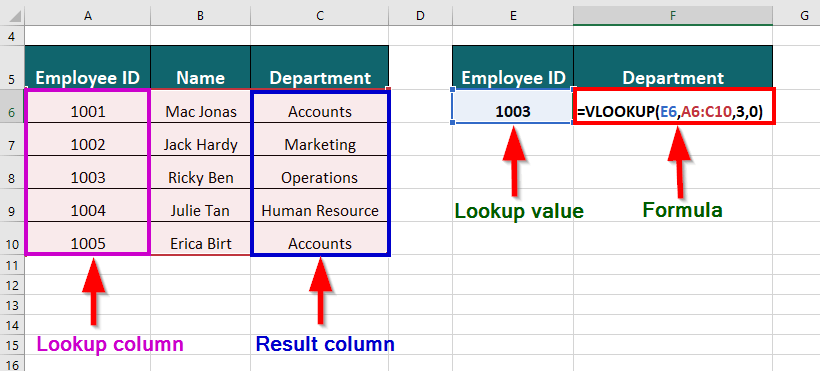
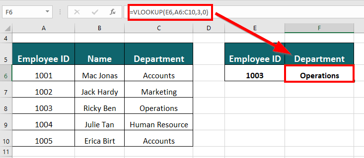
For example, you have a table consisting of a list of employee IDs, names, and the departments of company employees. The formula to find the Department of Persons having Employee ID 1003 is,
=VLOOKUP(E6,A6:C10,3,0)
Result = Operations
2. Sum Function
The SUM function in Excel provides the sum or addition of values of a selected cell range. The values can be numbers, ranges, arrays, and cell references. The values can be numbers, ranges, arrays, and cell references. The SUM function can add up to 255 values.
SUM Function Syntax:
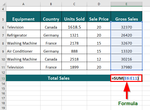
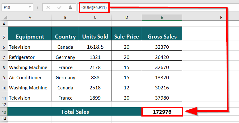
For example, if you want to find the sum of Gross sales on electronic equipment made by certain countries, the formula is =SUM(E6:E11)
Result= 172976
3. MAX Function
The MAX function in Excel provides the largest or maximum numeric value in the cell range. It ignores empty cells, text values, and the logical values TRUE and FALSE.
MAX Function Syntax:
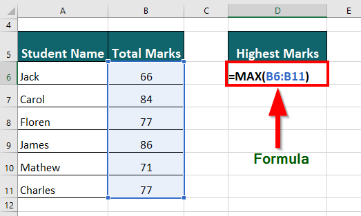
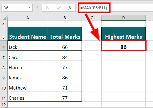
For example, if we want to find the highest marks from a list of student’s scores, the formula is =MAX(B6:B11)
Result= 86
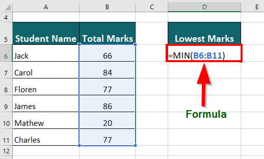
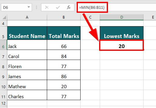
4. MIN Function
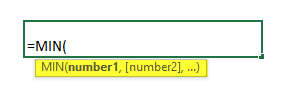
The MIN function in Excel provides the minimum or lowest numeric value in the cell range. It ignores empty cells, text values, and the logical values TRUE and FALSE.
For example, if we want to find the lowest marks from a list of student’s marks, the formula is =MIN(B6:B11)
Result= 20
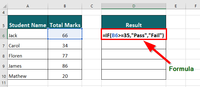
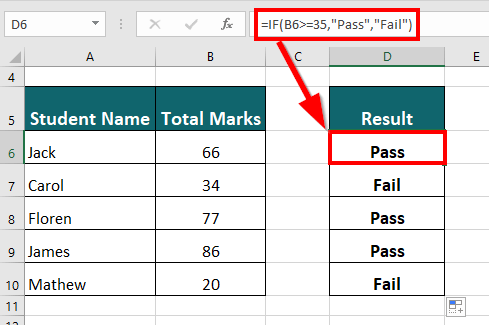
5. IF Function
The IF() function is a logical function in Excel that evaluates a specific condition and provides a particular value if the condition is True and another value if it’s False.
For example, if we want to test if a student has passed or failed an exam test based on criteria, the formula is =IF(B6>=35,”Pass”,”Fail”)
Result = Pass
Drag the formula into the other cells to get the result for the remaining cells.
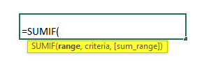
6. SUMIF Function
SUMIF in Excel function provides the sum of values of a specific cell range based on the given criteria.
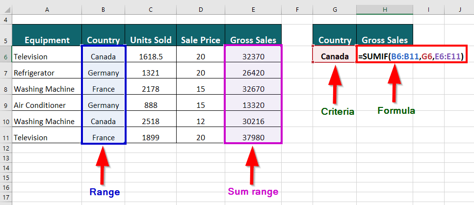
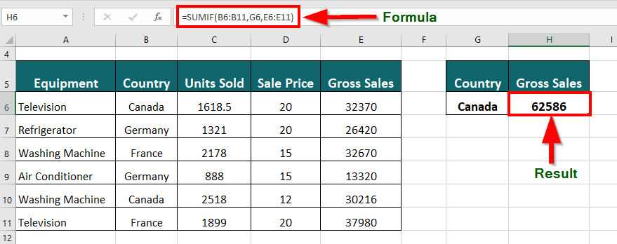
For example, if you want to add Gross sales made by Canada on specific electronic equipment, the formula is =SUMIF(B6:B11,G6,E6:E11)
Result = 62586
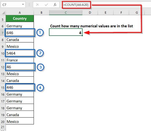
7. COUNT Function
The COUNT in Excel is a function that counts the number of cells that consists of numeric values in a selected range and ignores all the other entries in the range.
COUNT function Syntax:
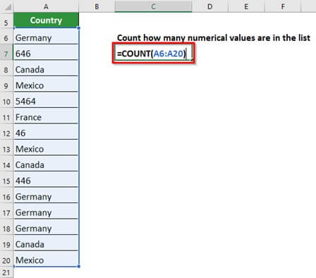
For example, if you have a list of countries with numerical codes and we want to find the total number of numerical codes from the given list, the formula is =COUNT(A6:A20)
Result = 4
8. COUNTIF Function
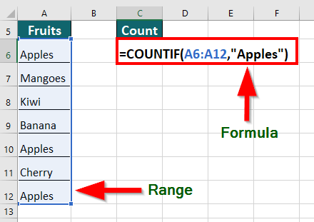
The COUNTIF function in Excel counts cells in a given range that meet a single criterion. We can use COUNTIF to count cells that contain numbers, texts, and dates.
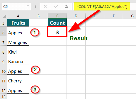
For example, if we want to count the number of apples from a given list of fruits, the formula is =COUNTIF(A6:A12,”Apples”)
Result= 3
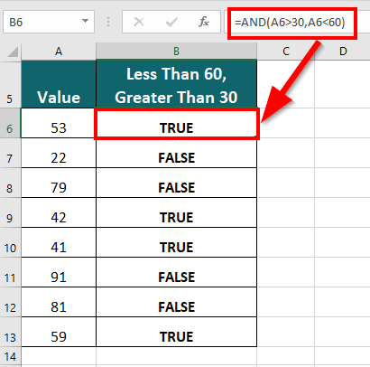
9. AND Function
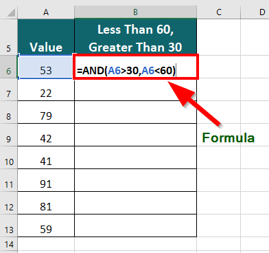
The AND function in Excel is a logical function that tests multiple criteria and returns either TRUE or FALSE.
For example, if we want to find if a given value is less than 60 and greater than 30, the formula is =AND(A6>30,A6<60)
Result = TRUE
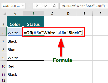
10. OR function
The function OR in Excel is structured as =OR(Condition1, Condition2,…) and performs logical tests by checking if any of the given conditions are true. If at least one of the conditions is true, the function returns TRUE; otherwise, it returns FALSE.
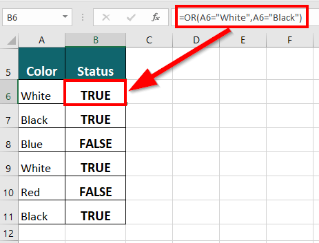
For example, if we want to test if a given color is White or Black, the formula will be
=OR(A6=”White”,A6=”Black”)
Result = TRUE
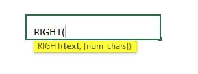
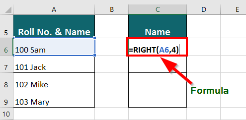
11. RIGHT Function
The RIGHT function in Excel provides the number of characters from the right of a given text string.
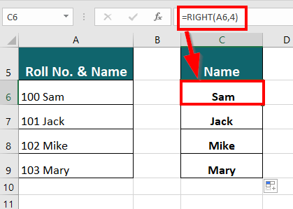
For example, we want to extract the name of students from a given list of Roll No. & Names, the formula is
=RIGHT(A6,4)
Result = Sam
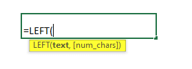
12. LEFT Function
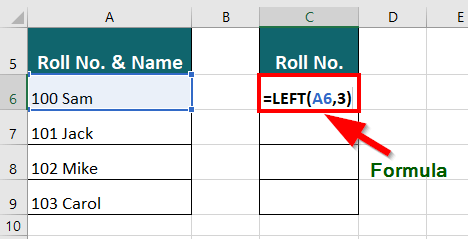
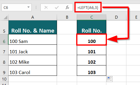
The LEFT function in Excel provides the number of characters from the left of a given text string.
For example, we want to extract the Roll no. of students from a given list of Roll No. & Names, the formula is
=LEFT(A6,3)
Result = 100
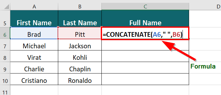
13. CONCATENATION Function
CONCATENATE in excel is an essential function that allows users to combine data from different cells and display the result in a single cell.
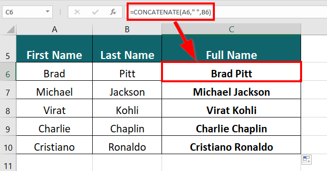
For instance, consider you have an Excel file with a long list of first and last names of clients written in different columns, and you want to display their full names in one column.
=CONCATENATE(A6,” “,B6)
Result = Brad Pitt
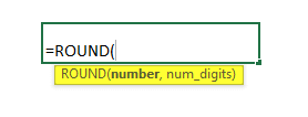
14. ROUND Function
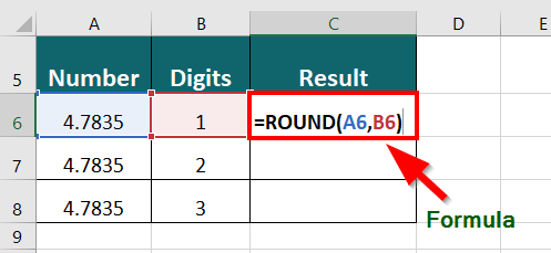
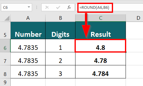
The ROUND function in Excel rounds up a numeric value to a given number of digits.
For example, to round the number 4.7835 to a given number of digits, the formula is =ROUND(A6,B6)
Result = 4.8
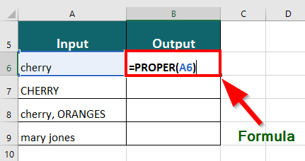
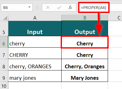
15. PROPER Function
The PROPER function in Excel capitalizes or changes the letters to uppercase in a given text string. The function does not affect numbers, spaces, and punctuation marks.
For example, if we want to change the appearance of a given text, the formula is
=PROPER(A6)
Result = Cherry
16. NOW Function
The Excel NOW function provides the date and time after making the data entry. The function edits the date and time every time the user opens or changes a worksheet.
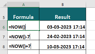
For example, the formula =NOW() gives the current date and time; =NOW()-7 gives the date and time 7 days before we made the entry, and =NOW()+7 gives the date and time 7 days ahead of the day when we made the entry.
17. Change the case
We can change the text’s case using Excel’s UPPER() and LOWER() functions.
SYNTAX
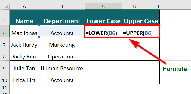
For example, if you have a list of employee names with their department and want to change the letter case of their department, the formula is
In case of lowercase, the formula is =LOWER(B6)
In case of uppercase, the formula is =UPPER(B6)
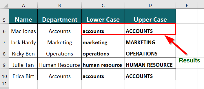
Result =
Lowercase = accounts
Uppercase = ACCOUNTS
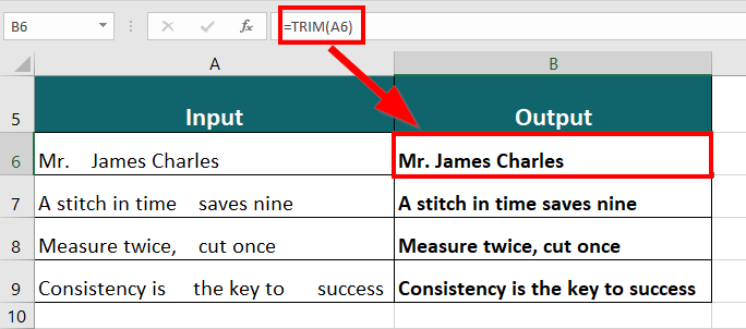
18. TRIM
The TRIM function in Excel removes any unwanted(extra) spaces between texts or at the beginning and end of a text.
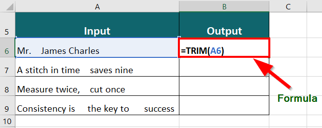
For example, the formula =TRIM(A6), removes any extra space from the given text
The result is Mr. James Charles
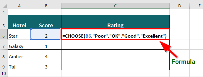
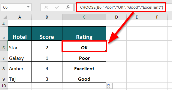
19. Choose()
The CHOOSE function in Excel provides a value from a list using a given index number or position.
For example, if we want to give a rating to a hotel using the given score, the formula is =CHOOSE(B6,”Poor”,”OK”,”Good”,”Excellent”)
Result = OK
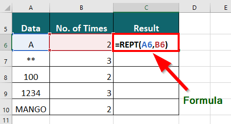
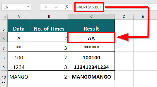
20. REPT()
The REPT function in Excel repeats characters a specified number of times.
For example, if we want the character A to appear twice, the formula is =REPT(A6,B6)
Result = AA
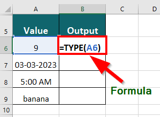
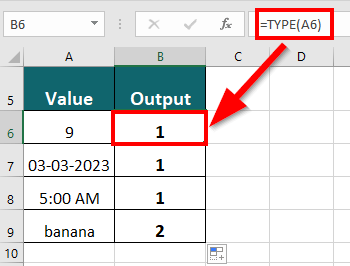
21. TYPE()
The TYPE function in excel provides a numeric value representing the data type. The numeric value for different data is: text = 2, number = 1, logical value = 4, error = 16, and array = 64.
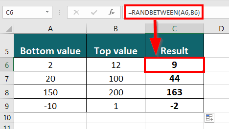
22. RANDBETWEEN()
This advanced excel formula lets you generate a random number between the two given values. It helps when you want to simulate results or behavior in spreadsheets.
For example, if you want to generate a random number between 2 and 12, the formula is =RANDBETWEEN(A6,B6)
Result = 9
Note: The RANDBETWEEN function recalculates the values each time you open or updates a worksheet.
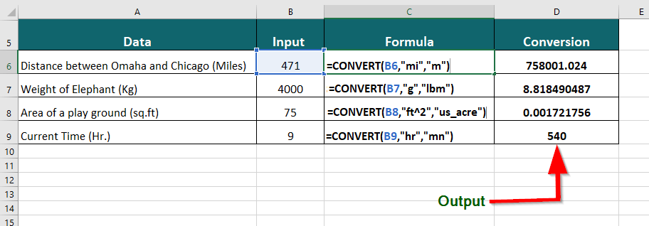
23. Unit conversion by CONVERT()
The CONVERT advanced excel formula converts a number from one measurement unit to another.
For example, the CONVERT can convert miles to meters, kilograms to pounds, square feet to the acre, hours to a minute, and more.
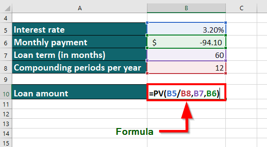
24. PV function
The PV function is a advanced excel formula that is a versatile virtual financial function that can calculate the rate, periods for investment, payment per period, future value, and other arguments based on the input of the variables.
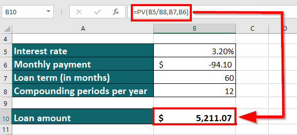
For example, if we want to calculate the loan amount from a given Interest rate, monthly payment, loan term, and compounding period, the formula is =PV(B5/B8,B7,B6).
Result = $ 5211.07
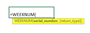
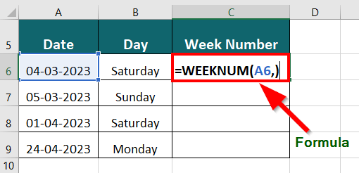
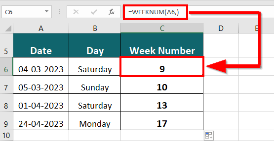
25. WEEKNUM Function
The WEEKNUM function in Excel evaluates a given date and provides a week number that corresponds to the week of the year. It starts counting on the week containing January 1.
For example, if you want to calculate the week number for the date 4th March 2023, the formula is =WEEKNUM(A6)
Result = 9
Conclusion
Microsoft Excel Advanced Formulas and Functions enable users to perform tasks as simple as adding numbers, calculating mortgage payments, creating financial models, and solving math and engineering problems.
Based on Excel’s trend results, marketing and product management must rely on foresight. As a result, the opportunities are limitless.
Frequently Asked Questions(FAQs)
Q1. What are the top 10 Excel formulas?
Answer: The Top 10 Excel formulas are:
#1 =VLOOKUP(lookup_value, table_array, colu_index_num, [range_lookup])
#2 =SUM(Number1, [Number2],…)
#3 =IF(logical_test, [value_if_true], [value_if_false])
#4 =SUMIF(range, criteria, [sum_range])
#5 =OR(logical1, [logical2],…)
#6 =CONCATENATE(text1, [text2],…)
#7 =CONVERT(number, from_unit, to_unit)
#8 =PV(rate, nper, pmt, [fv], [type])
#9 =COUNTIF(range, criteria)
#10 =AND(logical1, [logical2],…)
Q2. What is the importance of studying advanced spreadsheet skills
Answer: Advanced spreadsheet skills help connect with the real-world application of mathematics. It allows users to organize, prepare graphs, calculate, and analyze data. These skills are essential to execute any task related to finance, budgeting, or to prepare student reports.
Q3. What are the advanced Excel skills for accountants?
Answer: The Advanced Excel skills that would be helpful for accountants are:
- Vlookup to find data from an extensive database
- Creating Pivot tables to prepare reports
- Using Data Validation to create drop-down lists
- Using Proper Cell Referencing
- Logical Analysis using IF, AND, and OR functions
Recommended Articles
Here are some articles that will help you to get more detail about Advanced Excel Formula and Function.
- Best Excel Shortcuts
- Basic Excel Formula
- Drop Down List in Excel
- Compatibility Mode in Excel
These are the top 10 excel functions that you need to learn in 2021. With these 10 functions you can unlock the power of Excel. Functions are the driving force behind Excel. They allow you to turn info into insights. Functions in Excel allow you to interpret and alter your data according to the conditions you set.
However, if you’re an Excel pro, this list isn’t for you. Our list goes over the basics — stuff everyone needs to know — and a few new things recently added by Microsoft.
Follow along and try these out yourself. The example data set is available here! We’ll be assuming the role of a car dealership owner.
The 10 Excel functions to use in 2021
1. IF
First of all, let’s start with a simple yet very useful function. The IF function allows you to compare two values and receive an output based on the answer.
Syntax
=IF(logical argument,value if true,value if false)
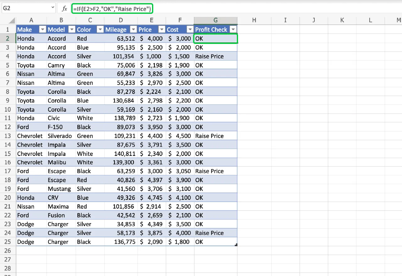
In our example, I want to know if the price we’ve listed for each car is greater than the cost we paid for it.
So our function is =IF(E2>F2,”OK”,”Raise Price”).
Basically, the =IF function allows you to set values for true and false. Here we’ve set it to read “OK” if our price is higher than our cost and “Raise Price” if we’ll lose money at the current price.
Let’s label our new column Profit Check. Include the quote-marks if you want to use a string of letters. Because if you don’t, Excel will think you’re entering a function and it won’t recognize it, creating a #NAME? error for unrecognized text.
Read more about the IF function on our blog.
2. SUM
Next up is the SUM function. It does exactly what you’d expect it to do. It sums the items in a specified range.
It’s usually the first function you learn when you open up Excel. It’s a great stepping stone for understanding how functions work.
Syntax
Remember that mathematics symbols can be inserted to change the function performed from adding to your desired operation.
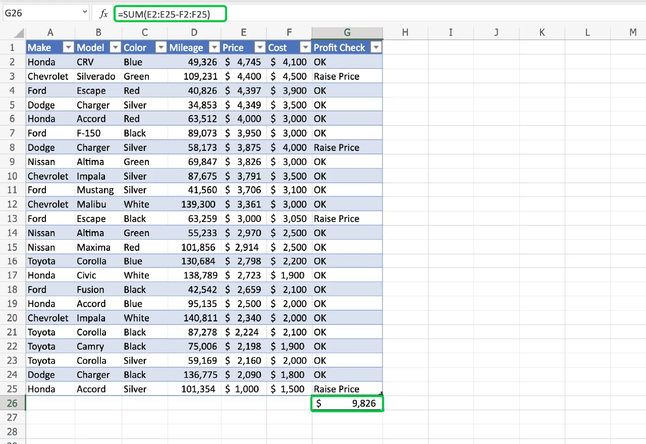
In our example, I want to know what our total profit will be if we sell all of our current inventory. This means that my function will be the range of our list price minus the range of our cost, written as =SUM(E2:E25-F2:F25).
As a result, the SUM function automatically totals the two ranges and subtracts the total cost from the total list price.
While SUM is simple — it’s just a basic math equation — It is a great time saver and shouldn’t be overlooked. It’s a quick way to understand your dataset.
3. SUBTOTAL
Similar to SUM, SUBTOTAL performs a function on a group of numbers.
Its power, however, comes from its modifiers. Depending on the modifier you include, SUBTOTAL can display the average, count, or rage of your data set, among other things.
The list of modifiers is available on Microsoft’s website.
Syntax
=SUBTOTAL(function modifier,number1,number2,…)
We want to know the average cost and list price for our inventory.
So our functions are =SUBTOTAL(101,E2:E25) and =SUBTOTAL(101,F2:F25).
When the SUBTOTAL function is used at the bottom of a table, a dropdown menu appears that lets you cycle through each of the operations it performs, making analysis a snap.
4. CONCAT
The CONCAT function joins, or concatenates, the inputs. It’s that simple.
You might have a list of first names and a list of last names, the CONCAT function will create a list of full names for you.
Syntax
If you want a space between elements, include a space between quote marks in your input list. It will look like this: (input1,” “,Input2).
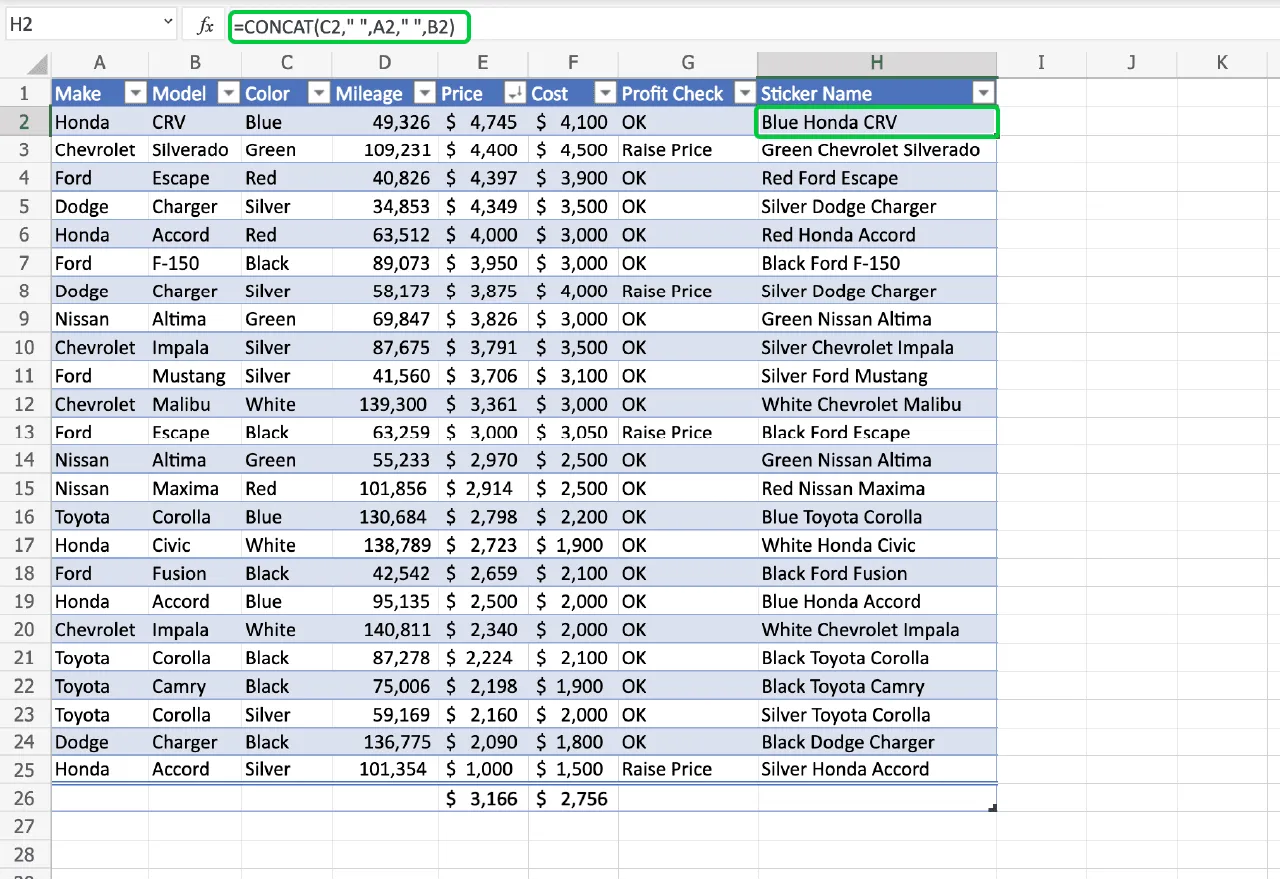
We want to make a column with the title of each car to post on our website. Because color, make, and model are all separate cells, we’re going to use the CONCAT function to make one cell with all of that information.
To do that we’ll write =CONCAT(C2,” “,A2,” “,B2). Make sure to include spaces in quotes between each element.
Let’s call our new column Sticker Name. Now we have a list of titles that we can hand over to our webmaster.
5. COUNTA
Similar to some previous Excel functions listed, the COUNTA function is another basic, but useful function. It simply counts. COUNTA will total the number of nonempty cells in a range.
It doesn’t matter if the cell contains a number, a string of letters, or an error, COUNTA will count it. On the other hand, if you only want a count of cells with number values, you can use =COUNT.
Syntax
=COUNTA(first cell in range:last cell in range)
If we want to have a running total of our inventory, we can use the COUNTA function for an entire Column.
To do that, we’ll write =COUNTA(A:A)-1 off to the side of our table. We include the minus one because the COUNTA function is counting our column label which we want to exclude.
Because COUNTA only counts cells with something in them, we can count the whole column and only get back the number of rows with information in them.
Now, when we update our inventory list, our inventory counter will update automatically. Put a label in front of our formula so you remember what the number represents.
6. COUNTIF
COUNTIF is related to COUNTA.
COUNTIF is a conditional counter, which means it only counts cells that fulfill an argument you give it.
Syntax
=COUNTIF(first cell in range:last cell in range,logical argument)
In this example, what if we wanted to know how many of the various brands of cars we have in stock. To do that we can use the COUNTIF function. Column A as our range. For the argument, if we put the model name in quotes, COUNTIF will only count the cells whose content matches the brand we’re interested in.
For example, our Honda counter is written =COUNTIF(A:A,”Honda”). We can create one for each of the models we carry, and make sure to label them.
Now we have a granular view of our inventory to go along with our general count.
7. UNIQUE
What if we don’t know all of the types of models we have in stock?
The UNIQUE function is useful in that situation. It creates a list of all of the unique values in a data set. It can also be used to make a list of values that only appear once.
Syntax
=UNIQUE(Array,By Column T/F, Exactly Once T/F)
By default it assumes that our data is organized in rows, and we want a list of the unique values in an array, but you can change that by setting the respective modifiers to true.
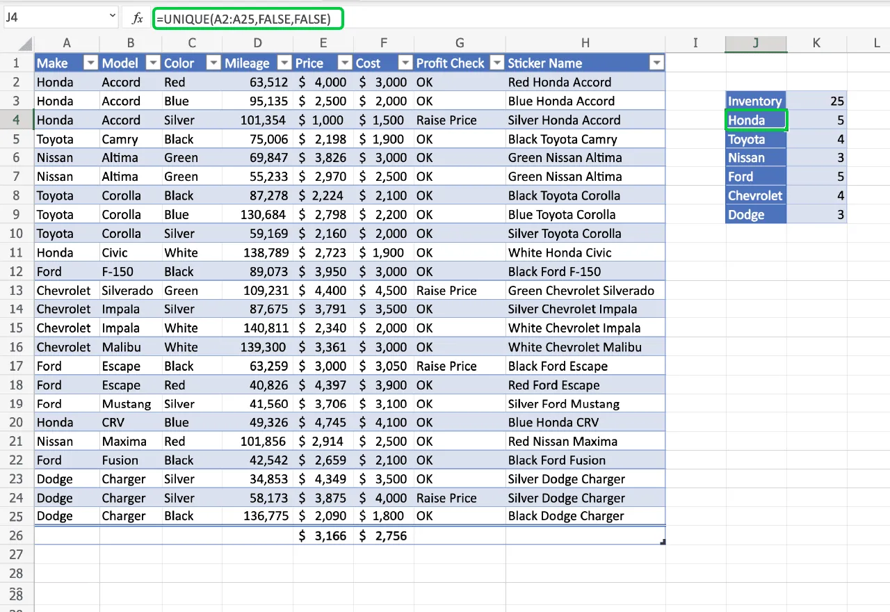
For our car dealership example, the UNIQUE function can replace the manually typed make names. In the first cell we type =UNIQUE(A2:A25). You don’t have to include the modifiers, they’ll automatically be set to false.
Now we’ve confirmed which brands we have in our inventory. Each brand is displayed once in our function’s list.
At this point we can update our COUNTIF functions by changing the brand name with the cell containing the brand in our new list. Now, anytime we reorder our list, or change a brand name, our inventory counter will update automatically.
8. SEQUENCE
On its surface, the SEQUENCE function doesn’t seem like it would be very useful. It only creates a list of numbers.
But when combined with other functions, it becomes a powerful tool.
Syntax
=SEQUENCE(number of row, number of columns,starting number, step size)
The SEQUENCE function assumes, if left blank, that columns, start number, and steps should be set to one.
Let’s assume we need to give each car in our list a unique identifying number. SEQUENCE can help us out. How can we make our sequence dynamic so that it automatically updates when we add or remove a vehicle from our stock? What if we reference our dynamic inventory counter from earlier to populate our sequence.
That would look like this: =SEQUENCE(L3). Let’s insert a new column on the left and title it ID Number.
Now each of our vehicles has a unique ID Number, that sets us up nicely for our next function.
9. XLOOKUP
If you’re familiar with Excel you might know the function VLOOKUP. Well, XLOOKUP is a new and improved version of VLOOKUP. If you want to read about VLOOKUP, check out our previous blog post here.
XLOOKUP works by matching a source to a cell in an array and returning information from a parallel array.
Syntax
=XLOOKUP(Lookup value,lookup array, return array,error message)
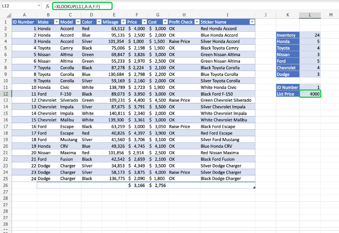
Back at the car dealership, let’s use XLOOKUP to find the price of a vehicle based on its ID Number. To do that we’ll write the ID Number we want to find in the cell above our XLOOKUP function.
That way we can reference the cell in our formula and easily change the ID Number we’re looking for. Our formula will be =XLOOKUP(L11,A:A,F:F).
If you go in and change the ID Number, the List Price will update automatically. This is a great tool for large datasets. Especially if everything has an ID or serial number.
10. FILTER
Now lastly, my favorite function, FILTER.
The FILTER function is like combining XLOOKUP and IF functions. It displays results based on conditions you provide.
Syntax
=FILTER(Array,Include If,error message)
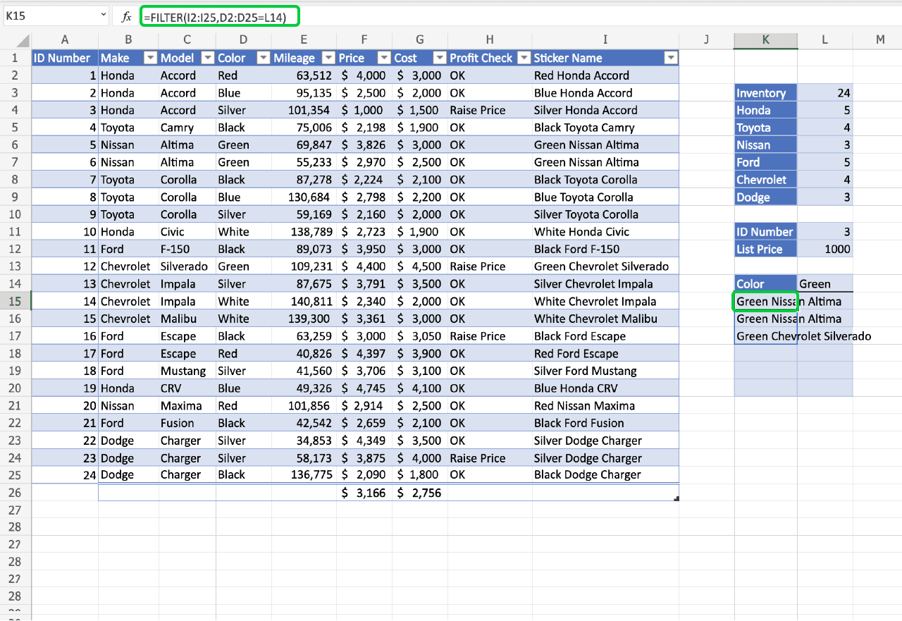
Searching our inventory for certain colors becomes easy with the FILTER function. We’ll write the color we’re interested in first so we can reference it in our function.
In the cell below that we’ll write our function, =FILTER(I2:I25,D2:D25=L14). We’re just pulling up the Sticker name in this example, but you can have it display as large of an array as you’d like.
Now you can type any color and pull up available models in that color. A great tool for salespeople who wanted to tell a client what is available in the color they want.
Final thoughts
With just these 10 functions we’ve created a handy little spreadsheet, saving our small business time. This isn’t a comprehensive list. Many more powerful Excel formulas exist.
To read up on some of them, check out the rest of our blog.
List of Top 10 Advanced Excel Formulas & Functions
You can download this Advanced Excel Formulas Template here – Advanced Excel Formulas Template
Table of contents
- List of Top 10 Advanced Excel Formulas & Functions
- #1 – VLOOKUP Formula in Excel
- #2 – INDEX Formula in Excel
- #3 – MATCH Formula in Excel
- #4 – IF AND Formula in Excel
- #5 – IF OR Formula in Excel
- #6 – SUMIF Formula in Excel
- #7 – CONCATENATE Formula in Excel
- #8 – LEFT, MID, and RIGHT Formula in Excel
- #9 – OFFSET Formula in Excel
- #10 – TRIM Formula in Excel
- Recommended Articles
#1 – VLOOKUP Formula in Excel
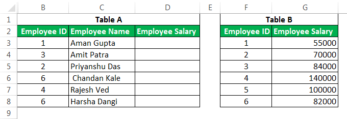
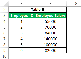
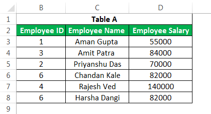
This advanced Excel function is one of the most used formulae in Excel. It is mainly due to the simplicity of this formula and its application in looking up a certain value from other tables, which has one standard variable across these tables. For example, suppose you have two tables detailing a company’s employee salary and name, with “Employee ID” being a primary column. You want to get the salary from Table B in Table A.
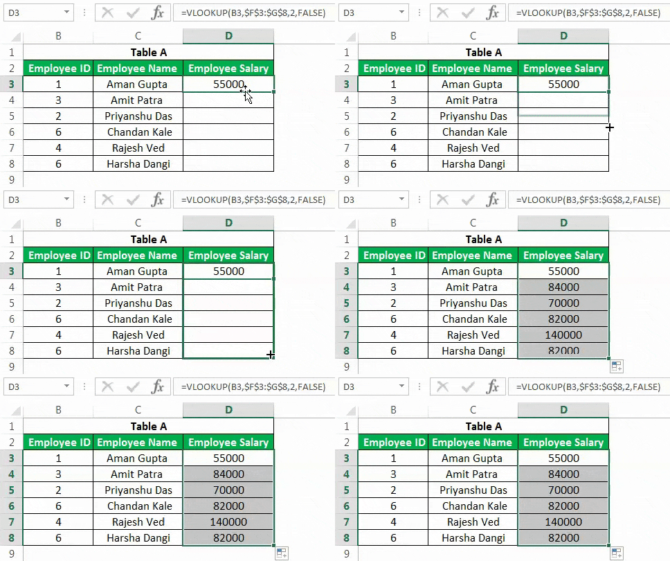
You can use VLOOKUPThe VLOOKUP excel function searches for a particular value and returns a corresponding match based on a unique identifier. A unique identifier is uniquely associated with all the records of the database. For instance, employee ID, student roll number, customer contact number, seller email address, etc., are unique identifiers.
read more as below.
It will result in the table below when we apply this advanced Excel formula in other cells of the “Employee Salary” column.
Drag the formula to the rest of the cells.
There are three major delimitations of VLOOKUP:
- You cannot have a primary column on the right of the column for which you want to populate the value from another table. The “Employee Salary” column cannot be before the “Employee ID.”
- In the duplicated values in the primary column in Table B, the first value will get populated in the cell.
- If you insert a new column in the database (e.g., insert a new column before “Employee Salary” in Table B), the output of the formula could be different based on the position that you have mentioned in the formula (in the above case, the result would be blank).
#2 – INDEX Formula in Excel
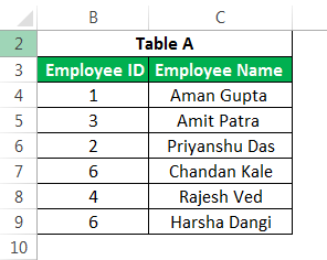
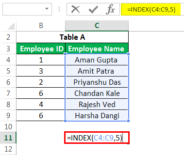
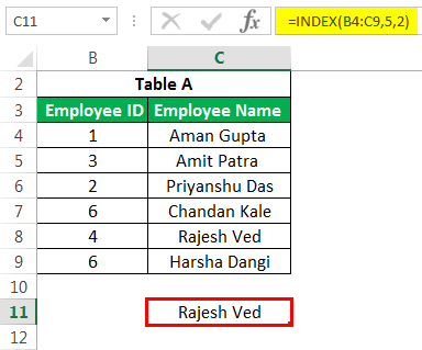
This advanced Excel formula is used to get the value of a cell in a given table by specifying the number of rows, columns, or both. E.g., to get an employee’s name at the 5th observation. Below is the data.
We can use the advanced Excel formula below:
We can use the same INDEX formula in getting values along the row. So, for example, when using both row and column numbers, the syntax would look like this:
The above formula would return as “Rajesh Ved.”
Note: If you insert another row into the 5th row, the formula will return as “Chandan Kale.” Hence, the output would depend on any changes in the data table over time.
#3 – MATCH Formula in Excel
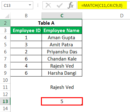
This Excel advanced formula returns the row or column number when a specific string or number is in the given range. In the below example, we are trying to find “Rajesh Ved” in the “Employee Name” column.
The formula would be as given below:
The MATCH functionThe MATCH function looks for a specific value and returns its relative position in a given range of cells. The output is the first position found for the given value. Being a lookup and reference function, it works for both an exact and approximate match. For example, if the range A11:A15 consists of the numbers 2, 9, 8, 14, 32, the formula “MATCH(8,A11:A15,0)” returns 3. This is because the number 8 is at the third position.
read more would return 5 as the value.
The 3rd argument is used for the exact match. You can also use +1 and -1 based on your requirements.
Note: One can combine INDEX and MATCH to overcome the limitation of VLOOKUP.
#4 – IF AND Formula in Excel
There are many instances when one needs to create flags based on some constraints. We all are familiar with the basic syntax of IF. We use this advanced excel IF functionIF function in Excel evaluates whether a given condition is met and returns a value depending on whether the result is “true” or “false”. It is a conditional function of Excel, which returns the result based on the fulfillment or non-fulfillment of the given criteria.
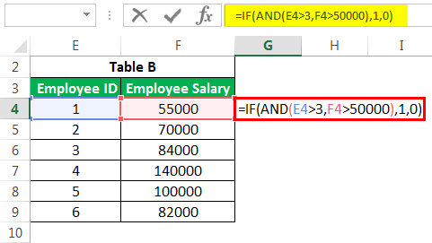
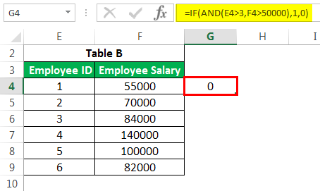
read more to create a new field based on some existing field constraints. But what if we need to consider multiple columns while creating a flag? E.g., in the below case, we want to flag all the employees whose salary is greater than 50,000. But “Employee ID” is greater than 3.
We would use the IF AND formula in such cases. Please find below the screenshot for the same.
It would return the result as 0.
We can have many conditions or constraints to create a flag based on multiple columns using AND.
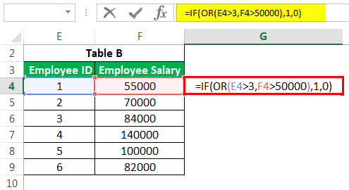
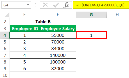
#5 – IF OR Formula in Excel
Similarly, we can use the OR function in ExcelThe OR function in Excel is used to test various conditions, allowing you to compare two values or statements in Excel. If at least one of the arguments or conditions evaluates to TRUE, it will return TRUE. Similarly, if all of the arguments or conditions are FALSE, it will return FASLE.read more instead of AND if we need to satisfy one of the many conditions.
If any condition is satisfied in the above cases, we will have the cell populated as 1, else 0. We can substitute 1 or 0 with some substrings with double quotes (“”).
#6 – SUMIF Formula in Excel
In some analyses, you might need to filter observations when applying the sum or count function. In such cases, this advanced Excel SUMIF function in excelThe SUMIF Excel function calculates the sum of a range of cells based on given criteria. The criteria can include dates, numbers, and text. For example, the formula “=SUMIF(B1:B5, “<=12”)” adds the values in the cell range B1:B5, which are less than or equal to 12.
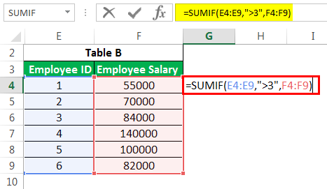
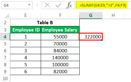
read more is at our rescue. It filters all the observations based on certain conditions in this advanced excel formula and sums up them. E.g., What if we want to know the sum of salaries of only those employees with employee IDs greater than 3?
By applying the SUMIFS formulaSUMIFS is an enhanced version of the SUMIF formula in Excel that enables you to sum any range of data by matching several criteria. read more:
The formula returns the results as 322000.
We can also count the number of employees in the organization having an employee ID greater than 3 using COUNTIF instead of SUMIF.
#7 – CONCATENATE Formula in Excel
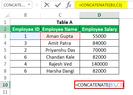
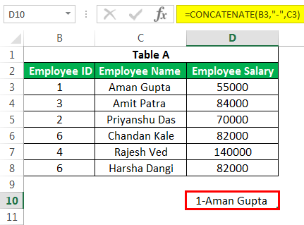
This Excel advanced function is one of the formulas used with multiple variants. This advanced Excel formula helps us join several text strings into one text string. For example, if we want to show “Employee ID” and “Employee Name” in a single column.
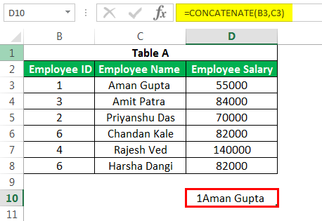
We can use this CONCATENATE formula here.
The above formula will result in “1Aman Gupta”.
We can have one more variant by putting a single hyphen between ID and NAME. E.g., CONCATENATE(B3,”-“,C3) will result in “1-Aman Gupta”. We can also use this in VLOOKUP when LOOKUP in ExcelThe LOOKUP excel function searches a value in a range (single row or single column) and returns a corresponding match from the same position of another range (single row or single column). The corresponding match is a piece of information associated with the value being searched.
read more value is a mixture of more than one variable.
#8 – LEFT, MID, and RIGHT Formula in Excel
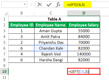
We can use this advanced Excel formula to extract a specific substring from a given string. One could use it based on our requirements. E.g., If we want to remove the first 5 characters from “Employee Name,” we can use the LEFT formula in ExcelThe left function returns the number of characters from the start of the string. For example, if we use this function as =LEFT ( «ANAND»,2), the result will be AN.read more with the column name and second parameter as 5.
The output is given below:
The application of the RIGHT formula in ExcelRight function is a text function which gives the number of characters from the end from the string which is from right to left. For example, if we use this function as =RIGHT ( “ANAND”,2) this will give us ND as the result.read more is also the same. It is just that we would be looking at the character from the right of the string. However, in the case of a MID function in excelThe mid function in Excel is a text function that finds strings and returns them from any mid-part of the spreadsheet. read more, we must give the required text string’s starting position and the string’s length.
#9 – OFFSET Formula in Excel
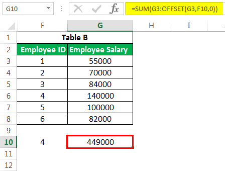
This advanced Excel function, combined with SUM or AVERAGE, could give a dynamic touch to the calculations. It is best used when we insert continuous rows into an existing database. OFFSET ExcelThe OFFSET function in excel returns the value of a cell or a range (of adjacent cells) which is a particular number of rows and columns from the reference point. read more provides a range where we need to mention reference cells, number of rows, and columns. E.g., If we want to calculate the average of the first 5 employees in the company where we have the salary of employees sorted by employee ID, we can do the following. The calculation below will always give us a salary.
- It will give us the sum of salaries of the first 5 employees.
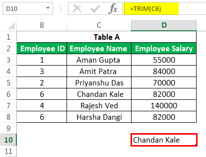
#10 – TRIM Formula in Excel
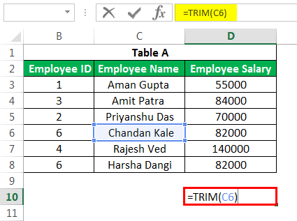
This advanced Excel formula is used to clean up the unimportant spaces in the text. E.g., if we want to remove spaces at the beginning of some name, we can use it by using the TRIM function in ExcelThe Trim function in Excel does exactly what its name implies: it trims some part of any string. The function of this formula is to remove any space in a given string. It does not remove a single space between two words, but it does remove any other unwanted spaces.read more as below:
The resultant output would be “Chandan Kale” without space before Chandan.
Recommended Articles
This article is a guide to Advanced Formulas in Excel. We discuss the top 10 Advanced Excel formulas and Advanced Excel functions with a downloadable template. You may learn more about Excel from the following articles: –
- Basic Excel Formulas
- VBA MID Function
- Match in Excel
- VLookup with IF


