
Hide error values and error indicators in cells
Excel for Microsoft 365 Excel 2021 Excel 2019 Excel 2016 Excel 2013 Excel 2010 Excel 2007 More…Less
Let’s say that your spreadsheet formulas have errors that you anticipate and don’t need to correct, but you want to improve the display of your results. There are several ways to hide error values and error indicators in cells.
There are many reasons why formulas can return errors. For example, division by 0 is not allowed, and if you enter the formula =1/0, Excel returns #DIV/0. Error values include #DIV/0!, #N/A, #NAME?, #NULL!, #NUM!, #REF!, and #VALUE!.
Convert an error to zero and use a format to hide the value
You can hide error values by converting them to a number such as 0, and then applying a conditional format that hides the value.
Create an example error
-
Open a blank workbook, or create a new worksheet.
-
Enter 3 in cell B1, enter 0 in cell C1, and in cell A1, enter the formula =B1/C1.
The #DIV/0! error appears in cell A1. -
Select A1, and press F2 to edit the formula.
-
After the equal sign (=), type IFERROR followed by an opening parenthesis.
IFERROR( -
Move the cursor to the end of the formula.
-
Type ,0) – that is, a comma followed by a zero and a closing parenthesis.
The formula =B1/C1 becomes =IFERROR(B1/C1,0). -
Press Enter to complete the formula.
The contents of the cell should now display 0 instead of the #DIV! error.
Apply the conditional format
-
Select the cell that contains the error, and on the Home tab, click Conditional Formatting.
-
Click New Rule.
-
In the New Formatting Rule dialog box, click Format only cells that contain.
-
Under Format only cells with, make sure Cell Value appears in the first list box, equal to appears in the second list box, and then type 0 in the text box to the right.
-
Click the Format button.
-
Click the Number tab and then, under Category, click Custom.
-
In the Type box, enter ;;; (three semicolons), and then click OK. Click OK again.
The 0 in the cell disappears. This happens because the ;;; custom format causes any numbers in a cell to not be displayed. However, the actual value (0) remains in the cell.
Use the following procedure to format cells that contain errors so that the text in those cells is displayed in a white font. This makes the error text in these cells virtually invisible.
-
Select the range of cells that contain the error value.
-
On the Home tab, in the Styles group, click the arrow next to Conditional Formatting and then click Manage Rules.
The Conditional Formatting Rules Manager dialog box appears. -
Click New Rule.
The New Formatting Rule dialog box appears. -
Under Select a Rule Type, click Format only cells that contain.
-
Under Edit the Rule Description, in the Format only cells with list, select Errors.
-
Click Format, and then click the Font tab.
-
Click the arrow to open the Color list, and under Theme Colors, select the white color.
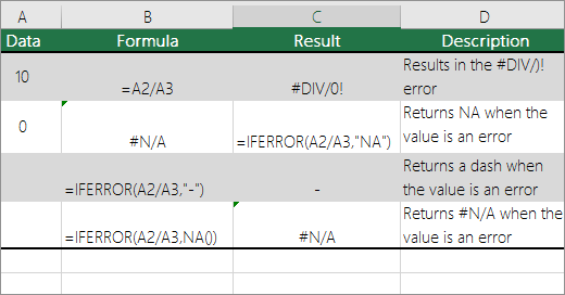
There may be times when you do not want error vales to appear in cells, and would prefer that a text string such as “#N/A,” a dash, or the string “NA” appears instead. To do this, you can use the IFERROR and NA functions, as the following example shows.
Function details
IFERROR Use this function to determine if a cell contains an error or if the results of a formula will return an error.
NA Use this function to return the string #N/A in a cell. The syntax is =NA().
-
Click the PivotTable report.
The PivotTable Tools appear. -
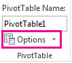
Excel 2016 and Excel 2013: On the Analyze tab, in the PivotTable group, click the arrow next to Options, and then click Options.
Excel 2010 and Excel 2007: On the Options tab, in the PivotTable group, click the arrow next to Options, and then click Options.
-
Click the Layout & Format tab, and then do one or more of the following:
-
Change error display Select the For error values show check box under Format. In the box, type the value that you want to display instead of errors. To display errors as blank cells, delete any characters in the box.
-
Change empty cell display Select the For empty cells show check box. In the box, type the value that you want to display in empty cells. To display blank cells, delete any characters in the box. To display zeros, clear the check box.
-
If a cell contains a formula that results in an error, a triangle (an error indicator) appears in the top-left corner of the cell. You can prevent these indicators from being displayed by using the following procedure.

Cell with a formula problem
-
In Excel 2016, Excel 2013, and Excel 2010: Click File > Options >Formulas.
In Excel 2007: Click the Microsoft Office Button
 > Excel Options > Formulas.
 -
Under Error Checking, clear the Enable background error checking check box.
 > Excel Options > Formulas.
Need more help?
At the time of using Excel formulas have you ever encountered error messages like #VALUE! or #DIV/0!? Do you know you can hide errors in Excel worksheet?
Well, the occurrence of such kinds of formula errors is a clear indication that you need to re-check the error source. Whereas in most cases such type of formula error simply shows that the data used by the formulas is not present.
Are you also the one who is looking for some easy tricks to hide error values in Excel? If you don’t know how Excel hide errors then this article is going to be very interesting and informative for you.
Following are some easy tricks to hide errors in Excel.
1# Hide Error Values In A PivotTable Report
2# Hide Error Indicators In Cells
3#Hide Error Values By Turning The Text White
4# Hide Errors With The IFERROR Function
5# Hide All Error Values In Excel With Conditional Formatting
Trick 1# Hide Error Values In A PivotTable Report
- Make a tap over the PivotTable report it will start showing PivotTable Tools.
- Excel 2016/2013: Go to the Analyze tab and then to the PivotTable Now hit the arrow sign present next to the Options, after that choose the Options button.
Excel 2010/2007: From the Options tab>PivotTable group. Hit the arrow sign present next to Options and after that choose the Options.
- Just hit the Layout & Format tab and try any of the following options:
- Change Error Display: From the Format tab choose the “For error values show”. In the appearing box, just assign the value which you want to show in place of errors.
In order to show errors like blank cells, just clear all the characters present in the box.
- Change Empty Cell Display:
From the Format tab choose the “For empty cells show” option. In the appearing box, just assign the value which you want to show in place of errors.
In order to show errors like blank cells, just clear all the characters present in the box. Whereas, to display zeros, just leave the check box empty.
Trick 2# Hide Error Indicators In Cells
If your cell is having a formula which is showing error then you will see a triangle single which is an error indicator. It appears in the cell’s top-left corner and one can easily stop these indicators from appearing by trying the following steps:
- Select the formula cell that is having the problem
- In Excel 2016/ 2013/ 2010: Hit the File> Options >Formulas.
In Excel 2007: Hit the Microsoft Office Button > Excel Options > Formulas.
- In the opened Error Checking dialog box, just clear the check box of Enable background error checking.

Trick 3# Hide Error Values By Turning The Text White
By applying the white color to your text you can easily hide errors in Excel. This will make your text color completely invisible.
- Choose the cells range that has the error value.
- Go to the Home tab and in the Styles group, tap to the arrow sign present next to the Conditional Formatting.

- After that hit the Manage Rules option. This will open the dialog box of Conditional Formatting Rules Manager.
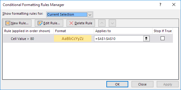
- Tap to the New Rule. After this, you will see a dialog box of New Formatting Rule will get open on your screen.
- From Select a Rule Type section hit the Format only cells that contain.
- Now from the Format only cells with section go to the Edit the Rule Description option and hit the Errors.
- Go to the Format tab, and then make a tap over the Font.
- For opening up, the Color list hit the arrow sign and then from the Theme Colors choose the white color.

Trick 4# Hide Errors With The IFERROR Function
The easiest trick to hide error values in the Excel workbook is by using the IFERROR function. So by making use of the IFERROR function one can very easily replace the error which is appearing with another value or also with the alternative formula.
In the given example, the VLOOKUP function is showing the #N/A error value.
Well, the error has occurred because there is no Office detail assigned for searching. Not only this, it will start causing issues with the total calculation.
The IFERROR function efficiently handles the error value such as, #NAME!, #DIV/0!, #REF! Etc. this needs a value for checking up the error and if the error is encountered what task needs to perform.
In the above-given example, the VLOOKUP function is used for checking up the values, and instead of error “0” will be displayed.
Trick 5# Hide All Error Values In Excel With Conditional Formatting
Excel Conditional Formatting function can also help you in the task of hiding error values. Follow the below-given steps:
1. Choose the data range up to which you are willing to hide the formula errors.
2 Follow this path: Home > Conditional Formatting > New Rule.

3. Now from the opened dialog box of New Formatting Rule you have to select ”Use a formula to determine which cells to format” option which is present within the “Select a Rule Type”.
After that enter the formula: =ISERROR(A1) within the text box of “Format values where this formula is true”. (A1 is 1st cell that is present within the selected range which you can modify as per your need)

4. Hit the Format button this will open the Format Cells dialog box. After that select a white color for cell font from the Font.
Tips: Try to keep the font and background color the same. Suppose you have selected a red color for your background then choose red color also for the font.

5. To close the opened dialog box hit the OK You will see that entire error values will goes hidden at once.


Best Software For Recover Missing Excel Workbook Data
If your Excel workbook data goes corrupted, missing, or deleted then you can make use of the MS Excel Repair Tool. This is the best tool to repair all sorts of issues, corruption, errors in Excel workbooks. This tool allows to easily restore all corrupt Excel file including the charts, worksheet properties cell comments, and other important data.
* Free version of the product only previews recoverable data.
This is a unique tool to repair multiple Excel files at one repair cycle and recovers the entire data in a preferred location. It is easy to use and compatible with both Windows as well as Mac operating systems. This software supports the entire Excel version.
Wrap Up:
Now that you know how to hide error in Excel then do try this in your worksheet.
I Hope this article seems informative to you. But if have any more tricks to share regarding this Excel hide errors techniques then feel free to share it with us on our Facebook and Twitter page.
Good Luck..!


Priyanka is an entrepreneur & content marketing expert. She writes tech blogs and has expertise in MS Office, Excel, and other tech subjects. Her distinctive art of presenting tech information in the easy-to-understand language is very impressive. When not writing, she loves unplanned travels.
С помощью условного форматирования можно скрывать нежелательные значения. Например, перед выводом документа на печать. Наиболее часто такими значениями являются ошибки или нулевые. Тем-более, эти значения далеко не всегда являются результатом ошибочных вычислений.
Как скрыть ошибки в Excel
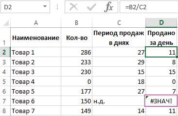
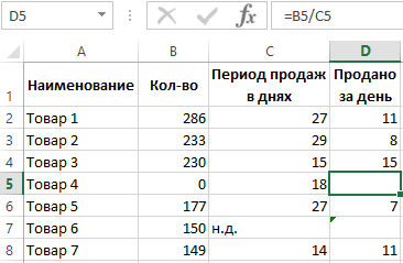
Чтобы продемонстрировать как автоматически скрыть нули и ошибки в Excel, для наглядности возьмем таблицу в качестве примера, в котором необходимо скрыть нежелательные значения в столбце D.
Чтобы скрыть ОШИБКУ в ячейке:
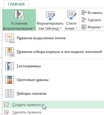
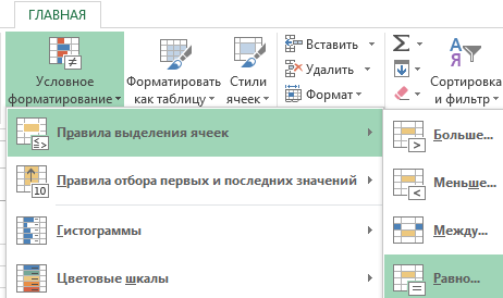
- Выделите диапазон ячеек D2:D8, а потом используйте инструмент: «ГЛАВНАЯ»-«Условное форматирование»-«Создать правило».
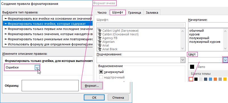
- В разделе данного окна «Выберите тип правила:» воспользуйтесь опцией «Форматировать только ячейки, которые содержат:».
- В разделе «Измените описание правила:» из левого выпадающего списка выберите опцию «Ошибки».
- Нажимаем на кнопку «Формат», переходим на вкладку «Шрифт» и в разделе «Цвет:» указываем белый. На всех окнах «ОК».
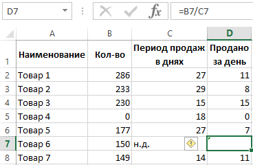
В результате ошибка скрыта хоть и ячейка не пуста, обратите внимание на строку формул.
Как скрыть нули в Excel
Пример автоматического скрытия нежелательных нулей в ячейках таблицы:
- Выделите диапазон ячеек D2:D8 и выберите инструмент: «ГЛАВНАЯ»-«Условное форматирование»-«Правила выделения ячеек»-«Равно».
- В левом поле «Форматировать ячейки, которые РАВНЫ:» вводим значение 0.
- В правом выпадающем списке выбираем опцию «Пользовательский формат», переходим на вкладку «Шрифт» и в разделе «Цвет:» указываем белый.

Документ не содержит ошибочных значений и ненужных нулей. Ошибки и нули скрыты документ готов к печати.
Общие принципы условного форматирования являются его бесспорным преимуществом. Поняв основные принципы можно приспособить решения к Вашей особенной задачи с минимальными изменениями. Эти функции в условном форматировании беспроблемно применяются для Ваших наборов данных, которые могут существенно отличаться от представленных на рисунках примеров.
While working with formulas in spreadsheets, we might get error values. These error values are often shown in the cells as error indicators. Sometimes, they are helpful in resolving errors but other times when errors need not be corrected, these error values just make the spreadsheet look cluttered. In such a situation, it is better to hide these error indicators to not only make the spreadsheet look clean but also to prevent these errors from stopping other formulas to work correctly. Let us discuss the different ways in which we can do that but first let us look at the problem statement with an example.
Hiding Error Values and Indicators in MS Excel
Open a new excel sheet and follow the steps given below.
Step 1: Go to the Math and Trig section on the formulas tab and click on the quotient option from the drop-down menu. You must see a pop-up like this:

Select the Quotient formula
Step 2: In this pop-up, enter 4 in the numerator and 0 in the denominator.

Enter values in the pop-up
Step 3: Click ok. You will get an error like this:

The div error
You can see how this error is indicated with an exclamatory mark since division by 0 is not defined. Some other error values can be #NAME?, #NULL!, and #REF!, etc.
Before we discuss the various ways in which we can hide these error values, let us first see how to deal with error indicators.
Change the Excel settings to Hide Error Indicators
As you can see in the above example, whenever a cell contains an error, a triangle appears in the top-left corner. This is nothing but an error indicator. Follow the steps given below to hide these error indicators:
Step 1: Go to file tab and select options.

Step 1
Step 2: A dialog box will appear. In this box, go to the formulas section and deselect the enable background checking box under the error checking section.

Step 2
Step 3: Click ok.
This was to hide the error indicators, now onto error values.
Use the IFERROR function to Convert the Error to Zero
Let us first enter =DIV(6/3) in the cell A1 of an excel spreadsheet.

Create an error
Then, click on enter and you will see an error like this:

#NAME error
To hide this error, follow the steps given below:
Step 1: Select cell A1 and click the F2 button. This is let you edit the formula.
Step 2: Now, to this formula, add the following function along with a 0 at the end as shown below.

IFERROR function
Step 3: Once you click enter, you will see a 0 in place of the #NAME? error.
If you wish, you can hide this 0 as well by using conditional formatting.
Hide the Zero with the help of the Conditional Format
Follow the below steps in continuation to hide the 0 present in cell A1.
Step 1: Select cell A1 and click on the conditional formatting option present under the home tab.

Conditional formatting option on the home tab
Step 2: From the list, select the New Rule option. You will see a dialog box like this:

New Rule Dialog box
Step 3: Inside this dialog box, select Format only cells that contain option from the rule type, and under the edit rule description section, the first cell should contain Cell value, the second cell should contain equal to and enter 0 in the last cell.

New Formatting rule
Step 4: Click the format button. You will see a dialog box with the name Format Cells appears. In this dialog box, click on the number tab, and select custom from the category section. Also, under the type section, enter three semicolons like this ;;; as shown below:

Format Cells
Step 5: Now, click ok. Click ok again. You can see that the 0 in cell A1 disappears after this.
We can also use the conditional formatting option to turn the text white so that the erroneous text is not visible.
Use Conditional format to turn text white and hide error values
To turn the text white using a conditional format, follow the below steps:
Note that we are using the same =DIV(6/3) error as above to explain this example.
Step 1: Select the cell or the range of cells containing error and click on the conditional formatting option present under the home tab.

Conditional formatting
Step 2: From the list, select the New Rule option. You will see a dialog box like this:
New formatting rule
Step 3: Inside this dialog box, select Format only cells that contain option from the rule type, and in the edit rule description section, select errors from the first dropdown.

New formatting rule
Step 4: Click on format. A new dialog box will appear. Go to the font section in this dialog box.

Font
Step 5: On the font tab, choose a white color from the color drop-down.

Color drop down
Step 6: Click ok. Click ok again.
Replace the Error with NA or a dash
We can use the IFERROR and NA functions to replace an error with the string NA, #N/A, or a dash(-).
The IFERROR function
The IFERROR function of excel is used to check if there is an error in a cell or a formula. If the error is found, the IFERROR function returns the value you specify. Otherwise, it simply returns the result of the formula.
Syntax
IFERROR(formula, replacement_value)
The function takes two arguments.
1. formula – It is the formula that has to be evaluated for errors.
2. replacement_value – It is the value that is returned when the formula evaluates to an error. The error can be #N/A, #REF!, #NULL!, #NAME?, #DIV/0! and #VALUE!.
Use the IFERROR function to replace the error with a dash or the string NA
Let us try this out on the first example error that we saw above.
Step 1: Double-click in cell A1 to edit the formula. Edit the formula as follows:

Edit the formula
Step 2: Press enter. You will see that the error is replaced by the string NA.

NA appears
If you want to display a dash instead of the string NA, then change the formula as follows:
=IFERROR(QUOTIENT(4,0), “-“)
The NA functions
This function simply returns #N/A. This is an error value that means ‘no value is available’. This helps in marking empty cells.
Syntax
NA()
This function has no arguments.
Use the NA function along with the IFERROR function to replace the error with #N/A
Just like we replaced an error value with a string or dash with the help of the IFERROR function, we can replace it with the value #N/A with the help of these two formulae:
=IFERROR(QUOTIENT(4,0), NA())
This is done below:
Step 1: Double-click in the cell A1 to edit the formula. Edit the formula as follows:

The formula
Step 2: Press Enter, and then you get the result.

The result

An error in Excel is a sign that a calculation or formula has failed to provide a result. You can hide Excel errors in a few different ways. Here’s how.
The perfect Microsoft Excel spreadsheet doesn’t contain errors—or does it?
Excel will throw out an error message when it can’t complete a calculation. There are a number of reasons why, but it’ll be up to you to figure it out and solve it. Not every error can be solved, however.
If you don’t want to fix the problem, or you simply can’t, you can decide to ignore the Excel errors instead. You might decide to do this if the error doesn’t change the results you’re seeing, but you don’t want to see the message.
If you’re unsure how to ignore all errors in Microsoft Excel, follow the steps below.
How to Hide Error Indicators in Excel
Used a formula incorrectly? Rather than return an incorrect result, Excel will throw up an error message. For example, you might see a #DIV/0 error message if you try to divide a value by zero. You may also see other on-screen error indicators, such as warning icons next to the cell containing the error.
You can’t hide the error message without altering the formula or function you’re using but you can hide the error indicator. This will make it less obvious that the spreadsheet data is incorrect.
To quickly hide error indicators in Excel:
- Open your Excel spreadsheet.
- Select the cell (or cells) containing the error messages.
- Click the warning icon that appears next to the cells when selected.
- From the drop-down, select Ignore Error.

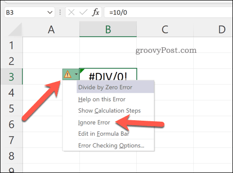
The warning icon will disappear, ensuring the error appears more discreetly in your spreadsheet. If you want to hide the error itself, you’ll need to follow the steps below.
How to Use IFERROR in Excel to Hide Errors
The best way to stop error messages from appearing in Excel is to use the IFERROR function. IFERROR uses IF logic to check a formula before returning a result.
For example, if a cell returns an error, return a value. If it doesn’t return an error, return the correct result. You can use IFERROR to hide error messages and make your Excel spreadsheet error-free (visually, at least).
The structure for an IFERROR formula is =IFERROR(value,value_if_error). You’ll need to replace value with a nested function or calculation that may contain an error. Replace value_if_error with the message or value that Excel should return instead of an error message.
If you’d rather see no error message appearing, use an empty text string (eg. “”) instead.
To use IFERROR in Excel:
- Open your Excel spreadsheet.
- Select an empty cell.
- In the formula bar, type your IFERROR formula (eg. =IFERROR(10/0,””)
- Press Enter to view the result.


IFERROR is a simple but powerful tool for hiding Excel errors. You can nest multiple functions within it, but to test it out, make sure the function you’re using is designed to return an error. If the error doesn’t appear, you’ll know it works.
How to Disable Error Reporting in Excel
If you want to disable error reporting in Excel completely, you can. This ensures that your spreadsheet remains free of errors, but you don’t need to use workarounds like IFERROR to do it.
You might decide to do this to prepare a spreadsheet for printing (even if there are errors). As your data might become incomplete or incorrect with error reporting disabled in Excel, we wouldn’t recommend disabling it for production use.
To disable error reporting in Excel:
- Open your Excel document.
- On the ribbon, press File.

- In File, press Options (or More > Options).

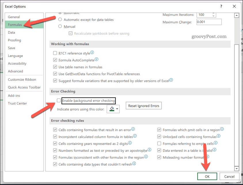
- In Excel Options, press Formulas.
- Uncheck the Enable background error checking checkbox.
- Press OK to save.


Resolving Issues in Microsoft Excel
If you’ve followed the steps above, you should be able to ignore all errors in an Excel spreadsheet. While it isn’t always possible to fix a problem in Excel, you don’t need to see it. IFERROR works well, but if you want a quick fix, you can always disable error reporting entirely.
Excel is a powerful tool, but only if it’s working properly. You may need to troubleshoot further if Excel keeps crashing, but an update or restart will usually fix it.
If you have a Microsoft 365 subscription, you can also try repairing your Office installation. If the file’s at fault, try repairing your document files instead.
![]()